✅ Week 04 Lab - Solutions

Tidymodel recipes and workflows - a tutorial

Author

Dr Stuart Bramwell and Dr Ghita Berrada

Instead of just reading the solutions, you might want to download the .qmd file and run the code yourself. You can download the .qmd file by clicking on the download button below:

📋 Lab Tasks

Part I - Getting Ready (10 min)

⚙️ Setup

Import required libraries:

# Remember to install.packages() any missing packages

# Tidyverse packages we will use
library(dplyr)     
library(ggplot2)
library(tidyr)     
library(readr)
library(stringr)
library(lubridate) 

# Tidymodel packages we will use
library(yardstick) # this is where metrics like mae() are
library(parsnip)   # This is where models like linear_reg() are
library(recipes)   # You will learn about this today
library(workflows) # You will learn about this today

# And finally a package for cleaning variable names
library(janitor)

Read the data set:

It is the same data set you used in the previous lab:

# Modify the filepath if needed
filepath <- "data/UK-HPI-full-file-2023-06.csv"
uk_hpi <- read_csv(filepath)

Rows: 136935 Columns: 54                                                                                                                                                                                                                              
── Column specification ───────────────────────────────────────────────────────────────────────────────────────────────────────────────────────────────────────────────────────────────────────────────────────────
Delimiter: ","
chr  (3): Date, RegionName, AreaCode
dbl (51): AveragePrice, Index, IndexSA, 1m%Change, 12m%Change, AveragePriceSA, SalesVolume, DetachedPrice, DetachedIndex, Detached1m%Change, Detached12m%Change, SemiDetachedPrice, SemiDetachedIndex, SemiDeta...

ℹ Use `spec()` to retrieve the full column specification for this data.
ℹ Specify the column types or set `show_col_types = FALSE` to quiet this message.

🎯 ACTION POINTS: Run the code chunk below, paying attention to what you are doing.

Let’s kick things off by crafting a df data frame that will hold records from select columns of the UK HPI dataset, broken down by individual UK countries. We’ll start our analysis from 2005 onwards.

df <-
  uk_hpi %>%
  clean_names() %>% 
  group_by(region_name) %>% 
  mutate(date = dmy(date),
         across(c(index, sales_volume), ~ lag(.x, 1), .names = "lag_1_{.col}")) %>%
  ungroup() %>% 
  filter(region_name %in% c("England", "Wales", "Scotland", "Northern Ireland"),
         date >= dmy("01-01-2005")) %>% 
  select(date, region_name, sales_volume, starts_with("lag_1"))

Let’s print out the first ten lines of our dataframe df to check the result of our code:

df  %>% head(10) %>% knitr::kable()

|date       |region_name | sales_volume| lag_1_index| lag_1_sales_volume|
|:----------|:-----------|------------:|-----------:|------------------:|
|2005-01-01 |England     |        53464|    78.81766|              80888|
|2005-02-01 |England     |        56044|    78.16973|              53464|
|2005-03-01 |England     |        67322|    78.18828|              56044|
|2005-04-01 |England     |        78958|    78.69753|              67322|
|2005-05-01 |England     |        79951|    79.53261|              78958|
|2005-06-01 |England     |        92080|    80.38431|              79951|
|2005-07-01 |England     |        96925|    80.87970|              92080|
|2005-08-01 |England     |        94592|    81.71145|              96925|
|2005-09-01 |England     |        96191|    82.04854|              94592|
|2005-10-01 |England     |        88571|    81.91431|              96191|

Part II - Tidymodels recipes (40 min)

🧑🏻‍🏫 TEACHING MOMENT: Your class teacher will explain all the code below. Follow along, running the code as you go. If you have any questions, don’t save it to later, ask away!

Say our goal is to predict sales_volume using the sales volume from the past month, similar to what we’ve been doing so far in this course, we could use dplyr functions mutate and lag to achieve that. That is:

df_train <-
    df %>% 
    group_by(region_name) %>%
    arrange(date) %>%
    mutate(SalesVolume_lag1 = lag(sales_volume, n=1)) %>% 
    drop_na()

# Then train it with tidymodels:
model <- 
    linear_reg() %>%
    set_engine("lm") %>%
    fit(sales_volume ~ ., data = df_train)

But today, we want to show you a different way of pre-processing your data before fitting a model!

We start with a recipe

Important

Note that the recipes libraries has a fair number of quirks.

You can read about some of those on our blogpost.

Another one is that it will, by default, set skip = TRUE for some steps (e.g step_naomit, which you’ll experiment with in this section) and any step with skip = TRUE is not applied to the data when bake() is called! So it is, in general, safer to set skip = FALSE to steps you add to ensure they are applied.

The problem with the code above is that, if you need to use the fitted model to make predictions on new data, you will need to apply the same pre-processing steps to that new data. This is not a problem if you are only doing it once, but if you need to do it many times, it can become a bit of a pain. This is where the recipes package (of tidymodels) comes in handy.

A recipe is a set of instructions of how the data should be pre-processed before it is used in a model. It is a bit like a cooking recipe, where you have a list of ingredients and a set of instructions on how to prepare them. In our case, the ingredient is the data frame, and the instructions are the pre-processing steps we want to apply to them.

Here’s how we would construct a recipe to pre-process our data before fitting a linear regression model:

# Create a recipe
rec <- 
  recipe(sales_volume ~ ., data = df) %>%
  step_naomit(lag_1_index, lag_1_sales_volume, skip = FALSE) %>%
  step_string2factor(region_name) %>% 
  update_role(date, new_role = "id") %>% 
  prep() 

summary(rec)

# A tibble: 5 × 4
  variable           type      role      source  
  <chr>              <list>    <chr>     <chr>   
1 date               <chr [1]> id        original
2 region_name        <chr [3]> predictor original
3 lag_1_index        <chr [2]> predictor original
4 lag_1_sales_volume <chr [2]> predictor original
5 sales_volume       <chr [2]> outcome   original

How do we use this recipe? Well, we can use the bake() function to apply the recipe to our data frame:

rec %>% 
  bake(df)

# A tibble: 883 × 5
   date       region_name lag_1_index lag_1_sales_volume sales_volume
   <date>     <fct>             <dbl>              <dbl>        <dbl>
 1 2005-01-01 England            78.8              80888        53464
 2 2005-02-01 England            78.2              53464        56044
 3 2005-03-01 England            78.2              56044        67322
 4 2005-04-01 England            78.7              67322        78958
 5 2005-05-01 England            79.5              78958        79951
 6 2005-06-01 England            80.4              79951        92080
 7 2005-07-01 England            80.9              92080        96925
 8 2005-08-01 England            81.7              96925        94592
 9 2005-09-01 England            82.0              94592        96191
10 2005-10-01 England            81.9              96191        88571
# ℹ 873 more rows
# ℹ Use `print(n = ...)` to see more rows

⚠️ If you don’t bake it, the pre-processing steps will not be applied. The recipe is just a recipe, not the final cooked meal. You need to bake it first.

How to use this in a model?

For this we need a workflow to which we can attach the recipe and the model. Creating a workflow of a linear regression looks like this:

# Create the specification of a model but don't fit it yet
lm_model <- 
  linear_reg() %>%
  set_engine("lm")

# Create a workflow to add the recipe and the model
wflow <- 
  workflow() %>% 
  add_recipe(rec) %>% 
  add_model(lm_model)

print(wflow)

══ Workflow ═══════════════════════════════════════════════════════════════════════════════════════════════════════════════════════════════════════════════════════════════════════════════════════════════════════
Preprocessor: Recipe
Model: linear_reg()

── Preprocessor ───────────────────────────────────────────────────────────────────────────────────────────────────────────────────────────────────────────────────────────────────────────────────────────────────
2 Recipe Steps

• step_naomit()
• step_string2factor()

── Model ──────────────────────────────────────────────────────────────────────────────────────────────────────────────────────────────────────────────────────────────────────────────────────────────────────────
Linear Regression Model Specification (regression)

Computational engine: lm

Then, you can fit the workflow to the data:

model <- 
  wflow %>% 
  fit(data = df)

model

══ Workflow [trained] ═════════════════════════════════════════════════════════════════════════════════════════════════════════════════════════════════════════════════════════════════════════════════════════════
Preprocessor: Recipe
Model: linear_reg()

── Preprocessor ───────────────────────────────────────────────────────────────────────────────────────────────────────────────────────────────────────────────────────────────────────────────────────────────────
2 Recipe Steps

• step_naomit()
• step_string2factor()

── Model ──────────────────────────────────────────────────────────────────────────────────────────────────────────────────────────────────────────────────────────────────────────────────────────────────────────

Call:
stats::lm(formula = ..y ~ ., data = data)

Coefficients:
                (Intercept)  region_nameNorthern Ireland          region_nameScotland             region_nameWales                  lag_1_index           lag_1_sales_volume  
                  20787.247                   -19073.839                   -17383.281                   -18738.808                       -9.527                        0.708

Do you want to confirm what recipe was used to pre-process the data? You can extract_recipe():

model %>% 
  extract_recipe()

── Recipe ─────────────────────────────────────────────────────────────────────────────────────────────────────────────────────────────────────────────────────────────────────────────────────────────────────────

── Inputs 
Number of variables by role
outcome:   1
predictor: 3
id:        1

── Training information 
Training data contained 888 data points and 9 incomplete rows.

── Operations 
• Removing rows with NA values in: lag_1_index, lag_1_sales_volume | Trained
• Factor variables from: region_name | Trained

Need to extract the fitted model? You can extract_fit_parsnip():

model %>% 
  extract_fit_parsnip()

parsnip model object


Call:
stats::lm(formula = ..y ~ ., data = data)

Coefficients:
                (Intercept)  region_nameNorthern Ireland          region_nameScotland             region_nameWales                  lag_1_index           lag_1_sales_volume  
                  20787.247                   -19073.839                   -17383.281                   -18738.808                       -9.527                        0.708

The output of the above is the same you would get if you had fitted the model directly using the fit() function (like we did last week). That is, you can use it to augment() the data with predictions:

fitted_model <- 
  model %>% 
  extract_fit_parsnip()

# To make predictions, I cannot use original data
# Instead, I have to apply the same pre-processing steps (i.e. bake the recipe)
df_baked <- 
  rec %>% 
  bake(df)

fitted_model %>% 
  augment(new_data = df_baked) %>% 
  head()

# A tibble: 6 × 7
   .pred  .resid date       region_name lag_1_index lag_1_sales_volume sales_volume
   <dbl>   <dbl> <date>     <fct>             <dbl>              <dbl>        <dbl>
1 77303. -23839. 2005-01-01 England            78.8              80888        53464
2 57894.  -1850. 2005-02-01 England            78.2              53464        56044
3 59720.   7602. 2005-03-01 England            78.2              56044        67322
4 67700.  11258. 2005-04-01 England            78.7              67322        78958
5 75930.   4021. 2005-05-01 England            79.5              78958        79951
6 76625.  15455. 2005-06-01 England            80.4              79951        92080

Notice that this augments our data frame with .pred and .resid columns.

How well did it perform, on average, by region? How does this compare to the standard deviation?

fitted_model %>% 
  augment(new_data = df_baked) %>% 
  group_by(region_name) %>%
  mae(truth = sales_volume, estimate = .pred) %>% 
  left_join(fitted_model %>% 
            augment(new_data = df_baked) %>% 
            group_by(region_name) %>% 
            summarise(sd = sd(sales_volume, na.rm = TRUE)),
            by = "region_name") %>% 
  pivot_longer(cols = c(.estimate, sd), names_to = "comp") %>% 
  ggplot(aes(x = value, y = region_name, fill = comp)) +
  geom_col(position = position_dodge()) +
  scale_fill_manual(values = c("black", "grey"), 
                    labels = c("MAE of Model", 
                               "Std. Dev. of Outcome")) +
  theme_bw() +
  theme(legend.position = "bottom") +
  labs(x = "Sales Volume", y = NULL, fill = NULL)

Let’s look at our residual plot across regions!

fitted_model %>% 
  augment(new_data = df_baked) %>% 
  mutate(.resid = .pred - sales_volume) %>% # only needed if augment() does not add a .resid column
  ggplot(aes(.pred, .resid)) +
  facet_wrap(. ~ region_name, scales = "free") +
  geom_point() +
  geom_hline(yintercept = 0, linetype = "dashed") +
  theme_bw() +
  labs(x = "Predicted sales volume", y = "Residuals")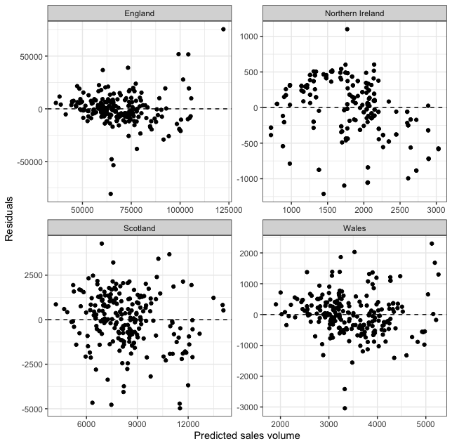

Part III - Practice with recipes and workflows (40 min)

Consider the following simulated data frame.


set.seed(123)

df_sim <-
  tibble(outcome = rnorm(100, 0, 1),
         feature1 = rnorm(100, 0, 1),
         feature2 = rnorm(100, 0, 20))

Let’s have a quick look at the first lines of df_sim before we proceed:

df_sim  %>% head(10) %>% knitr::kable()

|    outcome|   feature1|   feature2|
|----------:|----------:|----------:|
| -0.5604756| -0.7104066|  43.976207|
| -0.2301775|  0.2568837|  26.248259|
|  1.5587083| -0.2466919|  -5.302901|
|  0.0705084| -0.3475426|  10.863881|
|  0.1292877| -0.9516186|  -8.286799|
|  1.7150650| -0.0450277|  -9.524938|
|  0.4609162| -0.7849045| -15.772057|
| -1.2650612| -1.6679419| -11.892345|
| -0.6868529| -0.3802265|  33.018149|
| -0.4456620|  0.9189966|  -1.080563|

We have created a data set with one outcome (creatively labeled outcome) and two features feature1 and feature2 where one variable has been assigned a standard deviation 20 times the size of the other variable. In some cases like linear regression, it will be okay to use outcome ~ feature1 + feature2 as a formula. However, with other models, variables with larger variation will play a disproportionate role. As a result, we can use standardization (a.k.a. normalization) to counter this issue. This involves subtracting the mean of the variable and dividing the result by the standard deviation. Create a recipe for this data frame using a step from the tidymodels manual, bake the recipe, and make use of graphs to demonstrate that the standardization process “worked”.


# Let's look at the distributions of each feature overlaid!

df_sim %>% 
  pivot_longer(-outcome, names_to = 'feature') %>% 
  ggplot(aes(value, fill = str_remove(feature, "feature"))) +
  geom_histogram(alpha = 0.75) +
  theme_bw() +
  labs(x = "Feature value", y = "Frequency", fill = "Feature")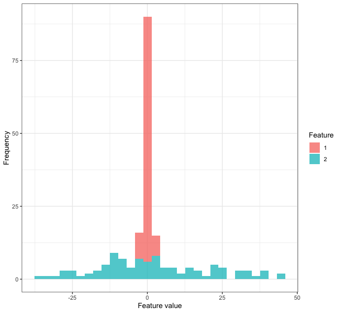

# Now let's normalize feature2 using step_normalize

df_normalized <-
  df_sim %>% 
  recipe(outcome ~ ., data = .) %>% 
  step_normalize(feature2) %>% 
  prep() %>% 
  bake(new_data = NULL)

# Now let's plot the distributions of the features

df_normalized %>% 
  pivot_longer(-outcome, names_to = 'feature') %>% 
  ggplot(aes(value, fill = str_remove(feature, "feature"))) +
  geom_histogram(alpha = 0.75) +
  theme_bw() +
  labs(x = "Feature value", y = "Frequency", fill = "Feature")

We have used recipes::step_string2factor to convert region_name from a string to a factor variable. However, some models will only require numeric input, meaning that we will have to convert this variable into several dummy variables. Using the tidymodels manual, can you find a step that can help us achieve this end?


# We can use step_dummy to achieve this end

df %>% 
  recipe(sales_volume ~ ., data = .) %>% 
  step_dummy(region_name) %>% 
  prep() %>% 
  bake(new_data = NULL)

# A tibble: 888 × 7
   date       lag_1_index lag_1_sales_volume sales_volume region_name_Northern.Ireland region_name_Scotland region_name_Wales
   <date>           <dbl>              <dbl>        <dbl>                        <dbl>                <dbl>             <dbl>
 1 2005-01-01        78.8              80888        53464                            0                    0                 0
 2 2005-02-01        78.2              53464        56044                            0                    0                 0
 3 2005-03-01        78.2              56044        67322                            0                    0                 0
 4 2005-04-01        78.7              67322        78958                            0                    0                 0
 5 2005-05-01        79.5              78958        79951                            0                    0                 0
 6 2005-06-01        80.4              79951        92080                            0                    0                 0
 7 2005-07-01        80.9              92080        96925                            0                    0                 0
 8 2005-08-01        81.7              96925        94592                            0                    0                 0
 9 2005-09-01        82.0              94592        96191                            0                    0                 0
10 2005-10-01        81.9              96191        88571                            0                    0                 0
# ℹ 878 more rows
# ℹ Use `print(n = ...)` to see more rows

Take a look at the following data frame.

df <-
  uk_hpi %>%
  clean_names() %>% 
  group_by(region_name) %>% 
  mutate(date = dmy(date),
         century = paste0(str_remove(as.character(year(date) + 100), "[0-9]{2}$"), "st"),
         across(c(index, sales_volume), ~ lag(.x, 1), .names = "lag_1_{.col}")) %>%
  ungroup() %>% 
  filter(region_name %in% c("England", "Wales", "Scotland", "Northern Ireland"),
         date >= dmy("01-01-2005")) %>% 
  select(date, century, region_name, sales_volume, starts_with("lag_1"))

We have created a variable that contains zero variance. Can you:

spot this variable (hint: check out dplyr::count) and

# Century is the offending variable

count(df, century)

# A tibble: 1 × 2
  century     n
  <chr>   <int>
1 21st      888

find an appropriate step in the tidymodels manual that can help us remove this variable?

# We can use step_select to remove it

df %>% 
  recipe(sales_volume ~ ., data = .) %>% 
  step_select(-century) %>% 
  prep() %>% 
  bake(new_data = NULL)

# A tibble: 888 × 5
   date       region_name lag_1_index lag_1_sales_volume sales_volume
   <date>     <fct>             <dbl>              <dbl>        <dbl>
 1 2005-01-01 England            78.8              80888        53464
 2 2005-02-01 England            78.2              53464        56044
 3 2005-03-01 England            78.2              56044        67322
 4 2005-04-01 England            78.7              67322        78958
 5 2005-05-01 England            79.5              78958        79951
 6 2005-06-01 England            80.4              79951        92080
 7 2005-07-01 England            80.9              92080        96925
 8 2005-08-01 England            81.7              96925        94592
 9 2005-09-01 England            82.0              94592        96191
10 2005-10-01 England            81.9              96191        88571
# ℹ 878 more rows
# ℹ Use `print(n = ...)` to see more rows

Using the data frame from step 2, create a recipe that incorporates Steps 1 and 2.


# We can simply combine steps 1. and 2.

new_rec <- 
  df %>% 
  recipe(sales_volume ~ ., data = .) %>% 
  step_select(-century) %>% 
  step_dummy(region_name) %>% 
  # Be sure to update the date column to an ID
  update_role(date, new_role = "id") %>% 
  prep()

new_rec

── Recipe ─────────────────────────────────────────────────────────────────────────────────────────────────────────────────────────────────────────────────────────────────────────────────────────────────────────────────────────────────────────────────────────────────────────────────────

── Inputs 
Number of variables by role
outcome:   1
predictor: 4
id:        1

── Training information 
Training data contained 888 data points and 9 incomplete rows.

── Operations 
• Variables selected: date, region_name, lag_1_index, lag_1_sales_volume, sales_volume | Trained
• Dummy variables from: region_name | Trained

Using the recipe in step 3, train a model that uses as training data only the records of England, Scotland and Wales. Calculate the Mean Absolute Error (MAE) of the training data. Then, respond: how does it compare to the MAE of the model trained on all UK countries (Part II)?


# Use the trusty dplyr::filter function

df_train <-
  df %>% 
  filter(region_name != "Northern Ireland")

# Whereas we have a new recipe, we can simply reuse the
# same instantiation of the linear model lm_model to 
# create our workflow.

new_wf <-
  workflow() %>% 
  add_recipe(new_rec) %>% 
  add_model(lm_model)

# All we need to do is fit the model, this time to the
# training data.

new_model <-
  new_wf %>% 
  fit(data = df_train)

# We can then extract the model object and show the
# MAE (or any other performance metric) that is 
# calculated using augment.

new_model %>% 
  extract_fit_parsnip() %>% 
  augment(new_data = bake(new_rec, df_train)) %>% 
  mae(truth = sales_volume, estimate = .pred)

# A tibble: 1 × 3
  .metric .estimator .estimate
  <chr>   <chr>          <dbl>
1 mae     standard       3755.

This is higher than the MAE of the model trained in Part II (i.e the model trained on all UK countries):

# A tibble: 1 × 3
  .metric .estimator .estimate
  <chr>   <chr>          <dbl>
1 mae     standard       2863.

This makes sense as the current model was trained on a data set containing less complete information than the dataset the model in Part II was trained on.

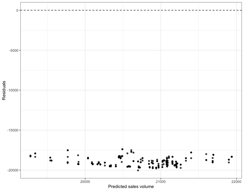
Now, let’s think of Northern Ireland records as a testing set. Predict sales_volume for Northern Ireland using the model you fitted in Step 2. Calculate the MAE of the predictions. What do you make of it?

# Pretty much the same code as above, only this
# time, we use == instead of != because we want
# Northern Ireland by itself.

df_test <-
  df %>% 
  filter(region_name == "Northern Ireland")

# Note that we use df_test the same way as df_train
# when we use augment.

new_model %>% 
  extract_fit_parsnip() %>% 
  augment(new_data = bake(new_rec, df_test)) %>% 
  mae(truth = sales_volume, estimate = .pred)

# A tibble: 1 × 3
  .metric .estimator .estimate
  <chr>   <chr>          <dbl>
1 mae     standard      18948.

The MAE is much worse here than the MAE of the model trained on the training set (i.e England+Scotland+Wales data) and obviously much worse than that of the model trained on all countries of the UK (Part II).

When compared to the model trained in Part II, our new model trained on Northern Ireland records was only trained on a subset of the data so predictably performs worse than a model that had complete information about the data set.

On the other hand, what the comparison between the model trained on Northern Ireland records only and the model trained on the other three UK countries reveals is (most likely) fundamentally different dynamics in the housing market in Northern Ireland compared to the rest of the UK. That might be worth a closer look!

Write a function called plot_residuals() that takes a fitted workflow model and a data frame in its original form (that is, before any pre-processing) and plot the residuals against the fitted values. The function should return a ggplot object.

plot_residuals <- function(wflow_model, data) {
    
    plot_df <-
      wflow_model %>% # This will be the model fitted with
                      # the workflow, not the workflow 
                      # itself!
      extract_fit_parsnip() %>% 
      augment(new_data = bake(new_rec, data))

    g <- 
      ggplot(plot_df, aes(x=.pred, y=.resid)) +
      geom_point(alpha = 0.75) +
      geom_hline(yintercept = 0, linetype = "dashed") +
      theme_bw() +
      labs(x = "Predicted sales volume", y = "Residuals")

    return(g)
    
}

Using the plot_residuals function you’ve just created, can you create:

one residuals against the fitted values plot for the training data used in Step 4
and another, separate residuals against the fitted values plot for the test data used in Step 5?

# We can call the function using df_train ...
plot_residuals(new_model, df_train)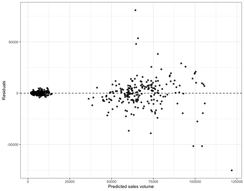

# ... and df_test

plot_residuals(new_model, df_test)