✅ Week 02 Lab - Solutions

2024/25 Winter Term

Author

The DS202 Team

Published

27 Jan 2025

This solution file follows the format of the Quarto file .qmd you had to fill in during the lab session.

Downloading the student solutions

Click on the below button to download the student notebook.

📋 Lab Tasks

🛠 Part 1: Data manipulation with `pandas` (45 min)

✨ `pandas` data frame attributes

A pandas data frame has a lot of attributes, several of which we shall explore:

shape: shows the number of rows and columns.
index: prints the name of each row in the data frame.
columns: prints the name of each column in the data frame.

🔧 `pandas` data frame methods

pandas data frames have a lot of methods! We will focus our attention on the following:

head / tail: shows the first / last n observations of a data frame.
to_frame: converts a series (pandas will automatically convert a data frame into a series if one variable is selected) to a data frame.
unique: shows all unique values for qualitative features selected.
value_counts: counts the number of times a unique value appears in a qualitative feature.
query: keeps rows that conform to one or more logical criteria.
reset_index: a subset of a data frame will keep the index of an old data frame. We use this method to change the index to one integer increments.
filter: keeps columns that are included in a user-supplied list (via the items parameter).
drop: drops columns that are included in a user-supplied list.
rename: renames already existing columns based on a user-supplied dictionary.
assign: creates a new variable based on a lambda function.
apply: applies a lambda function across a set of variables.
get_dummies: transforms qualitative features into a series of dummy features.
groupby: perform grouped calculations within qualitative features.

⚙️ Setup

Import required libraries:

import numpy as np
import pandas as pd
from lets_plot import *
LetsPlot.setup_html()

Import gapminder

gapminder = pd.read_csv("data/gapminder.csv")

1.1: Printing `pandas` data frames

Let’s print gapminder.

# Printing the object itself
print(gapminder)

# Printing the first 5 rows
print(gapminder.head(5))

# Printing the last 5 rows
print(gapminder.tail(5))

          country continent  year  lifeExp       pop   gdpPercap
0     Afghanistan      Asia  1952   28.801   8425333  779.445314
1     Afghanistan      Asia  1957   30.332   9240934  820.853030
2     Afghanistan      Asia  1962   31.997  10267083  853.100710
3     Afghanistan      Asia  1967   34.020  11537966  836.197138
4     Afghanistan      Asia  1972   36.088  13079460  739.981106
...           ...       ...   ...      ...       ...         ...
1699     Zimbabwe    Africa  1987   62.351   9216418  706.157306
1700     Zimbabwe    Africa  1992   60.377  10704340  693.420786
1701     Zimbabwe    Africa  1997   46.809  11404948  792.449960
1702     Zimbabwe    Africa  2002   39.989  11926563  672.038623
1703     Zimbabwe    Africa  2007   43.487  12311143  469.709298

[1704 rows x 6 columns]
       country continent  year  lifeExp       pop   gdpPercap
0  Afghanistan      Asia  1952   28.801   8425333  779.445314
1  Afghanistan      Asia  1957   30.332   9240934  820.853030
2  Afghanistan      Asia  1962   31.997  10267083  853.100710
3  Afghanistan      Asia  1967   34.020  11537966  836.197138
4  Afghanistan      Asia  1972   36.088  13079460  739.981106
       country continent  year  lifeExp       pop   gdpPercap
1699  Zimbabwe    Africa  1987   62.351   9216418  706.157306
1700  Zimbabwe    Africa  1992   60.377  10704340  693.420786
1701  Zimbabwe    Africa  1997   46.809  11404948  792.449960
1702  Zimbabwe    Africa  2002   39.989  11926563  672.038623
1703  Zimbabwe    Africa  2007   43.487  12311143  469.709298

We can see the dimensions of our data by calling the shape attribute of gapminder.

gapminder.shape

(1704, 6)

Here, we find that gapminder has 1,704 rows and 6 columns.

1.2: Data frames and series

We can see that gapminder has a list of countries and continents. We will explore continents further. To select only the continent column, we quote the variable name inside brackets next to gapminder.

gapminder["continent"]

0         Asia
1         Asia
2         Asia
3         Asia
4         Asia
         ...  
1699    Africa
1700    Africa
1701    Africa
1702    Africa
1703    Africa
Name: continent, Length: 1704, dtype: object

You can also reference variables using .:

gapminder.continent

0         Asia
1         Asia
2         Asia
3         Asia
4         Asia
         ...  
1699    Africa
1700    Africa
1701    Africa
1702    Africa
1703    Africa
Name: continent, Length: 1704, dtype: object

👉 NOTE: If you have variables separated by any white space or variables that contain special characters such as - or @, you can only use the brackets notation to select a column. The . (dot) notation can only be used for column names that are valid Python identifiers (e.g., no spaces, must start with a letter or underscore, and contain only alphanumeric characters or underscores).

This changes the data frame to a series. If you want the output to remain a data frame, however, you can use the to_frame method.

gapminder["continent"].to_frame()

continent
0         Asia
1         Asia
2         Asia
3         Asia
4         Asia
...        ...
1699    Africa
1700    Africa
1701    Africa
1702    Africa
1703    Africa

[1704 rows x 1 columns]

1.3: Finding / counting unique values

To find the names of all the continents we can use the unique method.

gapminder["continent"].unique()

array(['Asia', 'Europe', 'Africa', 'Americas', 'Oceania'], dtype=object)

To see how many times each continent appears, we can use the value_counts method. We use reset index in order to turn continent into its own column.

gapminder["continent"].value_counts().reset_index()

continent  count
0    Africa    624
1      Asia    396
2    Europe    360
3  Americas    300
4   Oceania     24

❓Question: Do you see anything odd?

Yes, there are only 24 observations for Oceania, despite the fact that gapminder contains multiple measurements of the same country from 1952 to 2007.

1.4: Performing grouped calculations

Suppose we want to calculate average GDP per capita across time. We can use a combination of the groupby and mean methods from Pandas.

gapminder.groupby("year", as_index=False)["gdpPercap"].mean()

year     gdpPercap
0   1952   3725.276046
1   1957   4299.408345
2   1962   4725.812342
3   1967   5483.653047
4   1972   6770.082815
5   1977   7313.166421
6   1982   7518.901673
7   1987   7900.920218
8   1992   8158.608521
9   1997   9090.175363
10  2002   9917.848365
11  2007  11680.071820

1.5: Subsetting rows

Suppose we want to investigate as to why Oceania has only 24 observations (see Part 1.3), we can start by using the query method, which filters rows by one or more conditions.

gapminder_oceania = gapminder.query("continent == 'Oceania'")

📝Task: Find the unique values of country in gapminder_oceania.

gapminder_oceania["country"].unique()

array(['Australia', 'New Zealand'], dtype=object)

❓Question: Do you see the reason now?

Yes, this is because only Australia and New Zealand are included in Oceania. No other island nations are included.

1.6: Subsetting columns

Suppose we only want our data frame to include country, year and population. We can use the filter method in a Pandas data frame setting the items parameter equal to a list of feature names that we want to include.

gapminder.filter(items=["country","year","pop"])

country  year       pop
0     Afghanistan  1952   8425333
1     Afghanistan  1957   9240934
2     Afghanistan  1962  10267083
3     Afghanistan  1967  11537966
4     Afghanistan  1972  13079460
...           ...   ...       ...
1699     Zimbabwe  1987   9216418
1700     Zimbabwe  1992  10704340
1701     Zimbabwe  1997  11404948
1702     Zimbabwe  2002  11926563
1703     Zimbabwe  2007  12311143

[1704 rows x 3 columns]

Another option is to use the drop method which takes a list of features to drop. Here, we specify axis=1 which signifies columns, not rows (to specify rows, we set axis=0).

gapminder.drop(["lifeExp","continent","gdpPercap"],axis=1)

country  year       pop
0     Afghanistan  1952   8425333
1     Afghanistan  1957   9240934
2     Afghanistan  1962  10267083
3     Afghanistan  1967  11537966
4     Afghanistan  1972  13079460
...           ...   ...       ...
1699     Zimbabwe  1987   9216418
1700     Zimbabwe  1992  10704340
1701     Zimbabwe  1997  11404948
1702     Zimbabwe  2002  11926563
1703     Zimbabwe  2007  12311143

[1704 rows x 3 columns]

Yet another way to achieve the same result as the filter and drop methods we’ve just shown is the double square bracket subsetting:

gapminder[["country","year","pop"]]

    country year    pop
0   Afghanistan 1952    8425333
1   Afghanistan 1957    9240934
2   Afghanistan 1962    10267083
3   Afghanistan 1967    11537966
4   Afghanistan 1972    13079460
... ... ... ...
1699    Zimbabwe    1987    9216418
1700    Zimbabwe    1992    10704340
1701    Zimbabwe    1997    11404948
1702    Zimbabwe    2002    11926563
1703    Zimbabwe    2007    12311143
1704 rows × 3 columns

👉 NOTE: If you have used pandas, you may have used the loc and iloc methods on data frames. These functions enable users to select both columns and rows in one function. While, in theory, this sounds great, these methods are computationally inefficient, so we advise that you do not use these methods and, instead, opt for query and filter or double square bracket subsetting.

1.7: Renaming columns

It is good practice to convert variable names to “snake case” whereby all characters are lower case and each word in the variable is separated by an underscore. To find the variable names expressed as an index, we call the columns attribute.

gapminder.columns

Index(['country', 'continent', 'year', 'lifeExp', 'pop', 'gdpPercap'], dtype='object')

From there, we can amend the variable names using a dictionary where the key is the current variable name and the value is the variable name you would like it to be. We then use the rename method, setting the columns parameter equal to the dictionary created.

# Create a dictionary of variable names using snake case
snake_case_var_names = {
  "country":"country",
  "continent":"continent",
  "year":"year",
  "lifeExp": "life_exp",
  "pop":"pop",
  "gdpPercap":"gdp_per_cap"
}

# Set the columns attribute to this list
gapminder = gapminder.rename(columns=snake_case_var_names)

# Check the columns attribute
gapminder.columns

Index(['country', 'continent', 'year', 'life_exp', 'pop', 'gdp_per_cap'], dtype='object')

1.8: Creating new variables

We know that Gross Domestic Product can be obtained from multiplying GDP per capita and population. To do this in Pandas, we simply insert * between the gdp_per_cap and pop columns found in gapminder.

gapminder["gdp"] = gapminder["gdp_per_cap"] * gapminder["pop"]
gapminder

country continent  year  life_exp       pop  gdp_per_cap  \
0     Afghanistan      Asia  1952    28.801   8425333   779.445314   
1     Afghanistan      Asia  1957    30.332   9240934   820.853030   
2     Afghanistan      Asia  1962    31.997  10267083   853.100710   
3     Afghanistan      Asia  1967    34.020  11537966   836.197138   
4     Afghanistan      Asia  1972    36.088  13079460   739.981106   
...           ...       ...   ...       ...       ...          ...   
1699     Zimbabwe    Africa  1987    62.351   9216418   706.157306   
1700     Zimbabwe    Africa  1992    60.377  10704340   693.420786   
1701     Zimbabwe    Africa  1997    46.809  11404948   792.449960   
1702     Zimbabwe    Africa  2002    39.989  11926563   672.038623   
1703     Zimbabwe    Africa  2007    43.487  12311143   469.709298   

               gdp  
0     6.567086e+09  
1     7.585449e+09  
2     8.758856e+09  
3     9.648014e+09  
4     9.678553e+09  
...            ...  
1699  6.508241e+09  
1700  7.422612e+09  
1701  9.037851e+09  
1702  8.015111e+09  
1703  5.782658e+09  

[1704 rows x 7 columns]

After having calculated GDP, you may be interested in coding whether or not a country has above median GDP. We can turn where in Numpy into a function and create a new column using the assign method.

# Returns a boolean array if a quantitative feature is above median values
def is_above_median(var):
  return np.where(var > np.median(var), True, False)

# Apply the function to GDP
gapminder[["country","year","gdp"]].assign(above_median = lambda x: is_above_median(x["gdp"]))

country  year           gdp  above_median
0     Afghanistan  1952  6.567086e+09         False
1     Afghanistan  1957  7.585449e+09         False
2     Afghanistan  1962  8.758856e+09         False
3     Afghanistan  1967  9.648014e+09         False
4     Afghanistan  1972  9.678553e+09         False
...           ...   ...           ...           ...
1699     Zimbabwe  1987  6.508241e+09         False
1700     Zimbabwe  1992  7.422612e+09         False
1701     Zimbabwe  1997  9.037851e+09         False
1702     Zimbabwe  2002  8.015111e+09         False
1703     Zimbabwe  2007  5.782658e+09         False

[1704 rows x 4 columns]

👉 NOTE: When using assign you can see that we use lambda x: followed by the function. All we are doing is using x as a placeholder for our data frame (country, year and gdp). In doing so, we can select the column we are interested in using to create our new boolean variable.

💁Tip: You may have noticed that we can string multiple methods together in Pandas. This is extremely useful, but you might find that your code will get too “long”. If you find this to be the case, you can use \ to spread your code over multiple lines. Here’s an example of how to do this with the above code:

gapminder[["country","year","gdp"]].\
    assign(above_median = lambda x: is_above_median(x["gdp"]))

country  year           gdp  above_median
0     Afghanistan  1952  6.567086e+09         False
1     Afghanistan  1957  7.585449e+09         False
2     Afghanistan  1962  8.758856e+09         False
3     Afghanistan  1967  9.648014e+09         False
4     Afghanistan  1972  9.678553e+09         False
...           ...   ...           ...           ...
1699     Zimbabwe  1987  6.508241e+09         False
1700     Zimbabwe  1992  7.422612e+09         False
1701     Zimbabwe  1997  9.037851e+09         False
1702     Zimbabwe  2002  8.015111e+09         False
1703     Zimbabwe  2007  5.782658e+09         False

[1704 rows x 4 columns]

📝Task: This output is not very helpful. Try using some of the commands we have gone over to create a more useful data frame.

gapminder[["country","year","gdp"]].\
  assign(above_median = lambda x: is_above_median(x["gdp"])).\
    query("above_median == True").\
      drop("above_median", axis=1).\
        reset_index(drop=True)

country  year           gdp
0    Afghanistan  2007  3.107929e+10
1        Algeria  1952  2.272563e+10
2        Algeria  1957  3.095611e+10
3        Algeria  1962  2.806140e+10
4        Algeria  1967  4.143324e+10
..           ...   ...           ...
847      Vietnam  2007  2.081746e+11
848  Yemen, Rep.  1992  2.512511e+10
849  Yemen, Rep.  1997  3.351236e+10
850  Yemen, Rep.  2002  4.179396e+10
851  Yemen, Rep.  2007  5.065987e+10

[852 rows x 3 columns]

1.9: Preparing data for `scikit-learn`, an example

📝Task: Filter the data to only include observations from 2007.

gapminder_07 = gapminder.query("year == 2007").reset_index(drop=True)
gapminder_07

country continent  year  life_exp       pop   gdp_per_cap  \
0           Afghanistan      Asia  2007    43.828  31889923    974.580338   
1               Albania    Europe  2007    76.423   3600523   5937.029526   
2               Algeria    Africa  2007    72.301  33333216   6223.367465   
3                Angola    Africa  2007    42.731  12420476   4797.231267   
4             Argentina  Americas  2007    75.320  40301927  12779.379640   
..                  ...       ...   ...       ...       ...           ...   
137             Vietnam      Asia  2007    74.249  85262356   2441.576404   
138  West Bank and Gaza      Asia  2007    73.422   4018332   3025.349798   
139         Yemen, Rep.      Asia  2007    62.698  22211743   2280.769906   
140              Zambia    Africa  2007    42.384  11746035   1271.211593   
141            Zimbabwe    Africa  2007    43.487  12311143    469.709298   

              gdp  
0    3.107929e+10  
1    2.137641e+10  
2    2.074449e+11  
3    5.958390e+10  
4    5.150336e+11  
..            ...  
137  2.081746e+11  
138  1.215686e+10  
139  5.065987e+10  
140  1.493170e+10  
141  5.782658e+09  

[142 rows x 7 columns]

📝Task: Create a list of numeric variables (life expectancy, population, GDP per capita, and GDP) and string variables (continent).

num_vars = ["life_exp","pop","gdp_per_cap","gdp"]
str_vars = ["continent"]

📝Task: Subset the new data frame to only include these variables. Remember you can add elements to a list by using +.

gapminder_07 = gapminder_07.filter(items=num_vars+str_vars)
gapminder_07

<life_exp       pop   gdp_per_cap           gdp continent
0      43.828  31889923    974.580338  3.107929e+10      Asia
1      76.423   3600523   5937.029526  2.137641e+10    Europe
2      72.301  33333216   6223.367465  2.074449e+11    Africa
3      42.731  12420476   4797.231267  5.958390e+10    Africa
4      75.320  40301927  12779.379640  5.150336e+11  Americas
..        ...       ...           ...           ...       ...
137    74.249  85262356   2441.576404  2.081746e+11      Asia
138    73.422   4018332   3025.349798  1.215686e+10      Asia
139    62.698  22211743   2280.769906  5.065987e+10      Asia
140    42.384  11746035   1271.211593  1.493170e+10    Africa
141    43.487  12311143    469.709298  5.782658e+09    Africa

[142 rows x 5 columns]

📝Task: Apply normalise to numeric variables

# Create a function that normalises variables
def normalise(var):
  return (var-var.mean())/var.std()

# Apply normalise function over all numeric variables
gapminder_07_normal = gapminder_07.filter(items=num_vars).\
  apply(lambda x: normalise(x), axis=0)

👉 NOTE: Normalising continuous features is good practice in machine learning, and becomes essential when dealing with algorithms that employ some kind of distance measure, such as principle components analysis.

Along with normalising features, we need to transform categorical features into one-hot encoded dummy (that is, 0 or 1) features. One-hot simply means that a reference category in a feature will not appear in the transformed data frame. To apply one-hot encoding, we can use get_dummies in Pandas.

gapminder_07_dummies = pd.get_dummies(gapminder_07["continent"], 
                                      columns=["continent"], 
                                      drop_first=True,
                                      dtype=int)
gapminder_07_dummies

Americas  Asia  Europe  Oceania
0           0     1       0        0
1           0     0       1        0
2           0     0       0        0
3           0     0       0        0
4           1     0       0        0
..        ...   ...     ...      ...
137         0     1       0        0
138         0     1       0        0
139         0     1       0        0
140         0     0       0        0
141         0     0       0        0

[142 rows x 4 columns]

After having transformed our continuous and categorical features, we can concatenate the two into a new data frame.

gapminder_07_cleaned = pd.concat([gapminder_07_normal, gapminder_07_dummies], axis=1)
gapminder_07_cleaned

life_exp       pop  gdp_per_cap       gdp  Americas  Asia  Europe  \
0   -1.919936 -0.082178    -0.832468 -0.288250         0     1       0   
1    0.779886 -0.273813    -0.446584 -0.295646         0     0       1   
2    0.438463 -0.072401    -0.424318 -0.153810         0     0       0   
3   -2.010799 -0.214066    -0.535216 -0.266522         0     0       0   
4    0.688525 -0.025195     0.085483  0.080659         1     0       0   
..        ...       ...          ...       ...       ...   ...     ...   
137  0.599815  0.279371    -0.718394 -0.153254         0     1       0   
138  0.531315 -0.270983    -0.672999 -0.302674         0     1       0   
139 -0.356947 -0.147739    -0.730898 -0.273324         0     1       0   
140 -2.039541 -0.218635    -0.809402 -0.300559         0     0       0   
141 -1.948180 -0.214807    -0.871728 -0.307533         0     0       0   

     Oceania  
0          0  
1          0  
2          0  
3          0  
4          0  
..       ...  
137        0  
138        0  
139        0  
140        0  
141        0  

[142 rows x 8 columns]

👉 NOTE: These kinds of transformations and concatenations will be employed a lot during this course, so please be sure to get used to them.

As a final (optional) step, we can convert our Pandas data frame to a Numpy array by employing the to_numpy method.

gapminder_07_cleaned.to_numpy()

array([[-1.91993566, -0.08217844, -0.8324684 , ...,  1.        ,
         0.        ,  0.        ],
       [ 0.77988582, -0.27381326, -0.446584  , ...,  0.        ,
         1.        ,  0.        ],
       [ 0.43846339, -0.07240145, -0.42431811, ...,  0.        ,
         0.        ,  0.        ],
       ...,
       [-0.35694651, -0.14773926, -0.73089796, ...,  1.        ,
         0.        ,  0.        ],
       [-2.03954118, -0.21863487, -0.8094021 , ...,  0.        ,
         0.        ,  0.        ],
       [-1.94818045, -0.21480678, -0.87172762, ...,  0.        ,
         0.        ,  0.        ]])

🏆Challenge: Which countries had above average life expectancy in 1952?

Try these steps: 1. Define a function that returns a boolean if a value in a feature exceeds the average value. 2. Include only the year 1952 by using query. 3. Subset the data frame to only include country and life expectancy using filter. 4. Create a new boolean variable using the user defined function using assign. 5. Include all rows with above average life expectancy using query. 6. Subset the data frame to only include country using square bracket indexing. 7. Pull the unique values into an array using unique.

# Returns a boolean array based on whether a quantitative feature has above average values
def is_above_average(var):
  return np.where(var > np.mean(var), True, False)

# Answer to be provided
gapminder.\
  query("year == 1952").\
    filter(items=["country","life_exp"]).\
      assign(above_average = lambda x: is_above_average(x["life_exp"])).\
        query("above_average == True")\
         ["country"].\
          unique()

array(['Albania', 'Argentina', 'Australia', 'Austria', 'Bahrain',
       'Belgium', 'Bosnia and Herzegovina', 'Brazil', 'Bulgaria',
       'Canada', 'Chile', 'Colombia', 'Costa Rica', 'Croatia', 'Cuba',
       'Czech Republic', 'Denmark', 'Finland', 'France', 'Germany',
       'Greece', 'Hong Kong, China', 'Hungary', 'Iceland', 'Ireland',
       'Israel', 'Italy', 'Jamaica', 'Japan', 'Korea, Dem. Rep.',
       'Kuwait', 'Lebanon', 'Mauritius', 'Mexico', 'Montenegro',
       'Netherlands', 'New Zealand', 'Norway', 'Panama', 'Paraguay',
       'Poland', 'Portugal', 'Puerto Rico', 'Reunion', 'Romania',
       'Serbia', 'Singapore', 'Slovak Republic', 'Slovenia', 'Spain',
       'Sri Lanka', 'Sweden', 'Switzerland', 'Taiwan', 'Thailand',
       'Trinidad and Tobago', 'United Kingdom', 'United States',
       'Uruguay', 'Venezuela'], dtype=object)

📋 Part 2: Data visualisation with `lets_plot`(45 min)

They say a picture paints a thousand words, and we are, more often than not, inclined to agree with them (whoever “they” are)! Thankfully, we can use perhaps the most widely used package, lets_plot (click here for documentation) to paint such pictures or (more accurately) build such graphs.

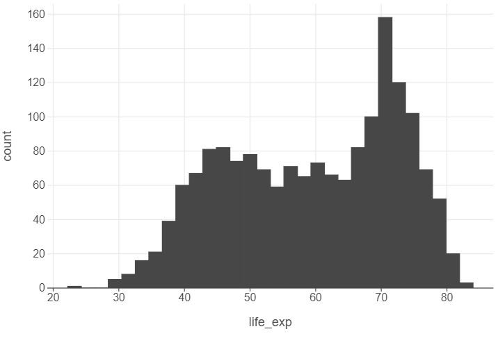
2.1 Histograms

Suppose we want to plot the distribution of an outcome of interest. We can use a histogram to plot the distribution of life expectancy in gapminder.

Tip

📝 Note: Step-by-step

If you are not familiar with using lets_plot for plotting, the line by line construction of the plot below might be useful. The + operator is used to add layers to the plot.

(
  ggplot(gapminder, aes("life_exp")) +
  geom_histogram()
)

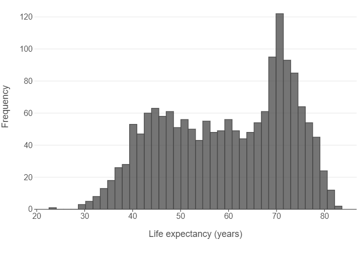
👥 WORK IN PAIRS/GROUPS:

Change a few parameters in the geom_histogram layer. - Set bins to 40. - Set alpha to 0.75.

Afterwards, - Specify panel_grid_major_x=element_blank() in the theme function. - Edit the x and y axes using labs.

(
  ggplot(gapminder, aes("life_exp")) +
  geom_histogram(alpha = 0.75, bins = 40) +
  theme(panel_grid_major_x=element_blank()) +
  labs(x = "Life expectancy (years)", y = "Frequency")
)

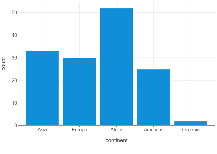
2.2 Bar graphs

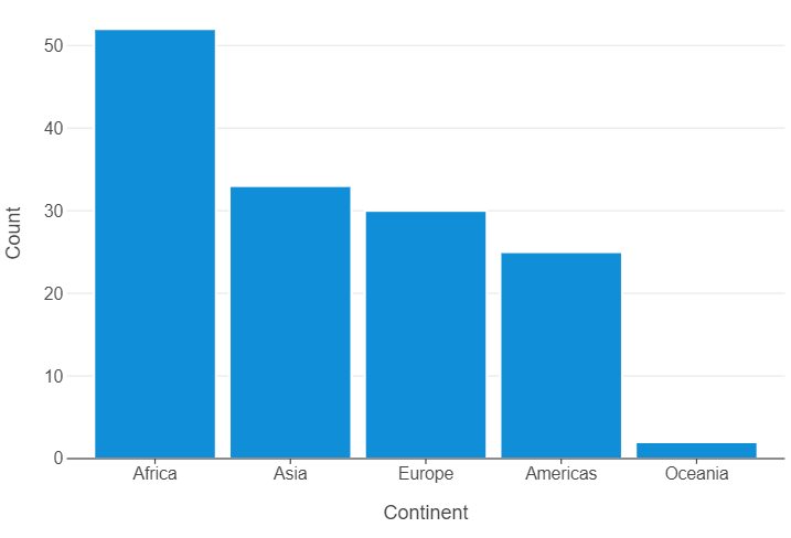
We counted the number of countries in each continent that are in gapminder. We will do something similar, using a subset of the data in 1997. We can use lets_plot to create a bar graph. We first need to specify what we want on the x and y axes, which constitute the first and second argument of the aes function.

gapminder_97 = gapminder.query("year == 1997")

(
  ggplot(gapminder_97,aes("continent")) +
  geom_bar()
)

👥 WORK IN PAIRS/GROUPS:

Create a new data frame that counts the number of observations for each continent.
Set stat="identity" in geom_bar.
Specify panel_grid_major_x=element_blank() in the theme function.
Edit the x and y axes using labs.

gapminder_97_count = gapminder_97.value_counts("continent").reset_index()

(
  ggplot(gapminder_97_count, aes("continent","count")) +
  geom_bar(stat="identity") +
  theme(panel_grid_major_x=element_blank()) +
  labs(x="Continent",y="Count")
)

👉 NOTE: Don’t like vertical bars? Well, we can also create horizontal bars too by specifying orientation="y" in geom_bar. Remember to switch “count” and “continent”.

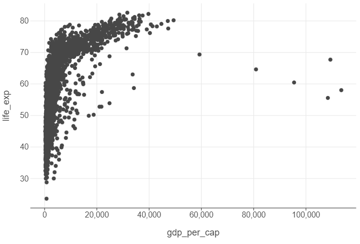
2.3 Scatter plots

Scatter plots are the best way to graphically summarise the relationship between two quantitative features. Suppose we wanted to visualise the “effect” of GDP per capita on life expectancy. We can use a scatter plot to achieve this.

(
  ggplot(gapminder, aes("gdp_per_cap","life_exp")) +
  geom_point()
)

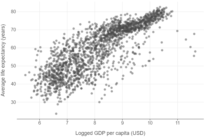
👥 WORK IN PAIRS/GROUPS:

Create a new feature that takes the natural log of GDP per capita.
Specify alpha=0.5 in geom_point.
Edit the x and y axes using labs.

gapminder["log_gdp_per_cap"] = np.log(gapminder["gdp_per_cap"])

(
  ggplot(gapminder, aes("log_gdp_per_cap","life_exp")) +
  geom_point(alpha=0.5) +
  labs(x="Logged GDP per capita (USD)", y = "Average life expectancy (years)")
)

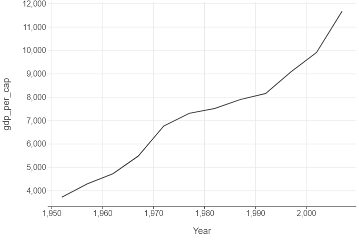
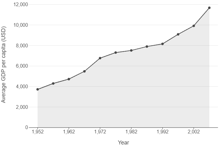
2.4 Line plots

Line plots can be used to track parameters of interest over time. We will do this by calculating then plotting average GDP per capita for each year.

gdp_per_cap_by_year = gapminder.groupby("year", as_index=False)["gdp_per_cap"].mean()

(
  ggplot(gdp_per_cap_by_year, aes("year", "gdp_per_cap")) +
  geom_line() +
  labs(x = "Year")
)

👥 WORK IN PAIRS/GROUPS:

Change linetype="dotted" in geom_line.
Add a geom_point and geom_area layer.
Change the breaks parameter in scale_x_continuous to an array from 1952 to 2007 by increments of 10.
Specify panel_grid_major_x=element_blank() in the theme function.
Edit the x and y axes using labs.

(
  ggplot(gdp_per_cap_by_year, aes("year", "gdp_per_cap")) +
  geom_line(linetype="dotted") +
  geom_point() +
  geom_area() +
  scale_x_continuous(breaks=np.arange(1952,2007,10)) +
  theme(panel_grid_major_x=element_blank()) +
  labs(x = "Year", y = "Average GDP per capita (USD)")
)

👉 NOTE: We think this line plot works in this context, and that it is useful to introduce you to this style of charting progress over time. However, for others contexts filling the area under the line may not work, so do bear this in mind when making decisions!

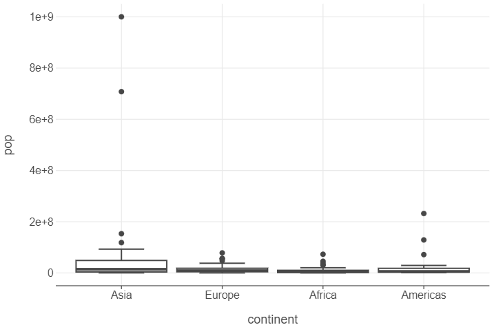
2.5 Box plots

Box plots are an excellent way to summarise the distribution of values across different strata over key quantities of interest (e.g. median, interquartile range). Suppose we want to show the distribution of populations by continent in gapminder in 1982 (excluding Oceania). We can use box plots to graphically illustrate this.

gapminder_oceania_82 = gapminder.query("continent != 'Oceania' & year == 1982")

(
  ggplot(gapminder_oceania_82, aes("continent", "pop")) +
  geom_boxplot() 
)

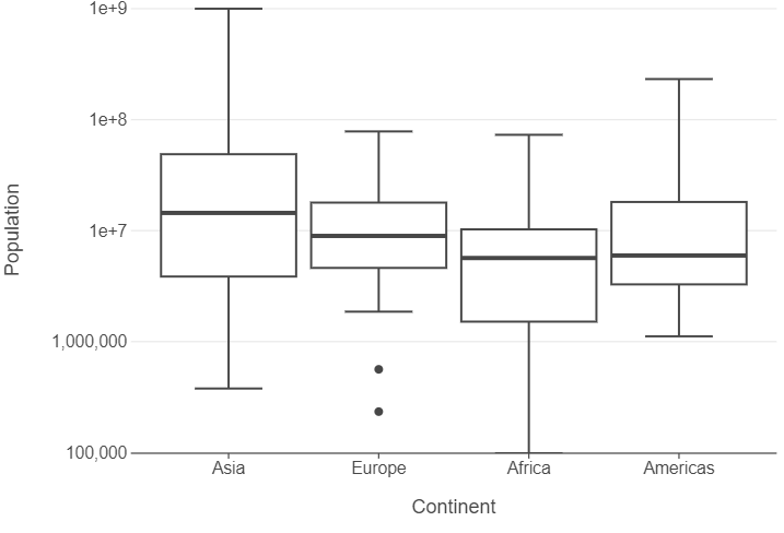
👥 WORK IN PAIRS/GROUPS:

Add scale_y_log10 to the plot.
Specify panel_grid_major_x=element_blank() in the theme function.
Edit the x and y axes using labs.

(
  ggplot(gapminder_oceania_82, aes("continent", "pop")) +
  geom_boxplot() +
  scale_y_log10() +
  theme(panel_grid_major_x=element_blank()) +
  labs(x="Continent", y="Population")
)

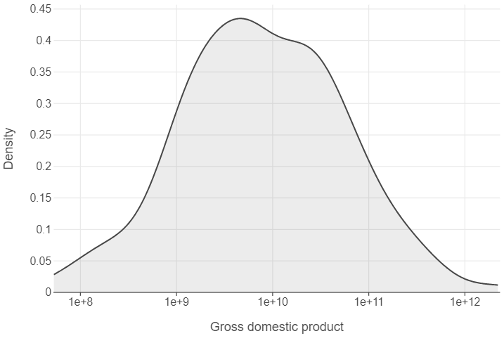
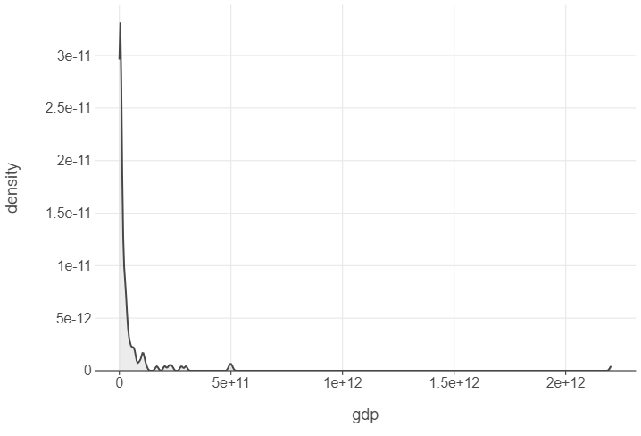
2.6 Density plots

Finally, we can understand the distribution of continuous features using density plots. Here’s an example that looks at the distribution of GDP in 1952.

gapminder_52 = gapminder.query("year == 1952")

(
  ggplot(gapminder_52, aes("gdp")) +
  geom_density() 
)

👥 WORK IN PAIRS/GROUPS:

Add scale_x_log10 to the plot.
Specify panel_grid_major_x=element_blank() in the theme function.
Edit the x and y axes using labs.

gapminder_52 = gapminder.query("year == 1952")

(
  ggplot(gapminder_52, aes("gdp")) +
  geom_density() +
  scale_x_log10() +
  labs(x="Gross domestic product", y="Density")
)

Downloading the student solutions

📋 Lab Tasks

🛠 Part 1: Data manipulation with pandas (45 min)

✨ pandas data frame attributes

🔧 pandas data frame methods

⚙️ Setup

1.1: Printing pandas data frames

1.2: Data frames and series

1.3: Finding / counting unique values

1.4: Performing grouped calculations

1.5: Subsetting rows

1.6: Subsetting columns

1.7: Renaming columns

1.8: Creating new variables

1.9: Preparing data for scikit-learn, an example

📋 Part 2: Data visualisation with lets_plot(45 min)

2.1 Histograms

2.2 Bar graphs

2.3 Scatter plots

2.4 Line plots

2.5 Box plots

2.6 Density plots

🛠 Part 1: Data manipulation with `pandas` (45 min)

✨ `pandas` data frame attributes

🔧 `pandas` data frame methods

1.1: Printing `pandas` data frames

1.9: Preparing data for `scikit-learn`, an example

📋 Part 2: Data visualisation with `lets_plot`(45 min)