
✅ Week 11 - Lab Solutions
Predicting true statements using the LIAR data set
This solution file follows the format of a Jupyter Notebook file .ipynb you had to fill in during the lab session.
👉 NOTE: We wanted to flag that this solution is far from optimal. Rather, it is more to serve as a demonstration of what kinds of analyses can be performed using this data set using the tools studied in DS202 (supervised learning part) or that extend them slightly (unsupervised part).
⚙️ Setup
Downloading the student solutions
Click on the below button to download the student notebook.
Loading libraries
import numpy as np
import pandas as pd
import spacy
from scipy.stats import mode
from sklearn.preprocessing import OneHotEncoder
from gensim.models.ldamodel import LdaModel
from gensim.models.coherencemodel import CoherenceModel
from sklearn.decomposition import LatentDirichletAllocation
import matplotlib.pyplot as plt
from gensim.models import Phrases
from gensim.models.phrases import Phraser
from gensim.corpora import Dictionary
from collections import Counter
from itertools import chain
from sklearn.model_selection import train_test_split, GridSearchCV
from sklearn.feature_extraction.text import CountVectorizer, TfidfVectorizer
from sklearn.metrics import confusion_matrix, f1_score, recall_score, precision_score
from sklearn.linear_model import LogisticRegression
from xgboost import XGBClassifier
from sklearn.decomposition import TruncatedSVD
import umap
from sklearn.cluster import SpectralClustering,AgglomerativeClustering
from sklearn.ensemble import IsolationForest
from sklearn.neighbors import LocalOutlierFactor
from sklearn.svm import OneClassSVM
from kmedoids import KMedoids
import plotly.express as px
from gower import gower_matrix
from tqdm import tqdm
import pyLDAvis
import networkx as nx
from scipy.sparse import csr_matrix
from skfuzzy.cluster import cmeans
from lets_plot import *
LetsPlot.setup_html()
import warnings
warnings.filterwarnings('ignore')
# Load spaCy stopwords
nlp = spacy.load("en_core_web_sm")
stopwords = nlp.Defaults.stop_words
%matplotlib inline
import os
from bertopic import BERTopic
from sentence_transformers import SentenceTransformer
Load the data set
We will start by loading liar and inspecting the distribution of the target. We find that approximately 42% of samples contain true statements, as defined in the Week 11 Lab Roadmap.
# Read the .csv
liar = pd.read_csv("../data/liar-dataset-cleaned-v2.csv")

# How is our target distributed?
liar.value_counts("true_statement").to_frame()

true_statement  count
0           False   3304
1            True   2436
Feature Selection: Statements
We’ll start by extracting features from the statements. The code for doing this is largely similar to the code provided in Week 10, but with two differences:
- We are creating n-grams, specifically unigrams and bigrams as features.
- We have specified a miminum document frequency of 15 to cut down on the number of features.
# Preprocess function: tokenize, remove punctuation, numbers, and stopwords
def preprocess_text(text):
    doc = nlp(text.lower())  # Lowercase text
    tokens = [
        token.lemma_ for token in doc
        if not token.is_punct and not token.is_digit and not token.is_space
        and token.text.lower() not in stopwords
    ]
    return " ".join(tokens)  # Return cleaned text as a string

# Apply preprocessing to each review
liar["statement_cleaned"] = liar["statement"].apply(preprocess_text)

# Create document-feature matrix (DFM) using CountVectorizer
vectorizer = CountVectorizer(min_df=15, ngram_range=(1,2))
dfm = vectorizer.fit_transform(liar["statement_cleaned"])

# Convert to a DataFrame for inspection
dfm = pd.DataFrame(dfm.toarray(), columns=vectorizer.get_feature_names_out())
Feature Selection: Contexts
Statements are made in many contexts, which might influence the statement maker’s propensity to tell the truth. We will build code that rationalises context by lumping all contexts that appear in 10 or less statements into an “other” category. To work with scikit-learn, we can transform this column into a one-hot encoded series of dummy variables.
# Create a count for each context
counts = liar.value_counts("context")

# Set the threshold
threshold = 10

# Create a variable that transforms the context column
liar["context_lumped"] = liar["context"].apply(lambda x: x if pd.notna(x) and counts.get(x, 0) >= threshold else "other")

# Convert the column to dummies
contexts = pd.get_dummies(liar["context_lumped"], columns=["context_lumped"], prefix="context")
Feature Selection: Subjects
As some subjects are more contentious than others, this might also influence a public figure’s propensity to tell the truth. subjects has already been transformed into dummies, so all we need to do is isolate them.
subjects = liar[liar.columns[liar.columns.str.contains("subj_")]]Constructing the training and testing set
# Concatenate the features into one set of features
X = pd.concat([dfm,subjects,contexts], axis=1)

# Isolate the target
y = liar["true_statement"]

# Perform the train test split
X_train, X_test, y_train, y_test = train_test_split(X, y, stratify=y, random_state=123)
Supervised Learning: Penalised logistic regression
Let’s try out some different combinations of hyperparameters. We will build a dictionary that has different kinds of penalties (l1 = Lasso, l2 = Ridge), along with different levels of penalty.
# Create a dictionary of hyperparameter choices
pl_params = {"penalty":["l1","l2"], "C": [0.5,0.1,0.01,0.001]}

# Instantiate a lasso classification model
logit_classifier = LogisticRegression(solver="liblinear",max_iter=1000,random_state=123)

# Instantiate a Grid Search
pl_grid = GridSearchCV(logit_classifier, param_grid=pl_params, scoring="f1", cv=10)

_ = pl_grid.fit(X_train, y_train)
Below, we can visualise which hyperparameter combination words best. We can see that at high levels of regularisation, Ridge tends to outperform Lasso considerably. However, when regularisation is relaxed, Lasso starts to slightly outperform Ridge.
(
    ggplot(pd.DataFrame(pl_grid.cv_results_), aes("param_C", "mean_test_score", color = "param_penalty")) +
    geom_point() +
    geom_line(linetype = "dashed") +
    theme(panel_grid_major_x=element_blank()) +
    labs(x = "Regularisation level", y = "Mean F1-Score", color = "Penalty Type",
         title = "A Lasso model with middling regularisation scores highest!")
)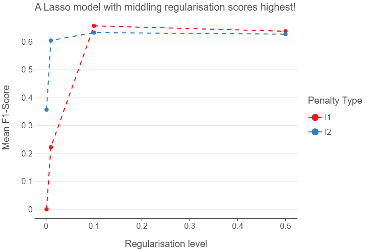
We can now apply our “optimal” hyperparameter combinations to the whole of the training set.
# Instantiate a lasso classification model
lasso_classifier = pl_grid.best_estimator_
# Fit the model to the training data
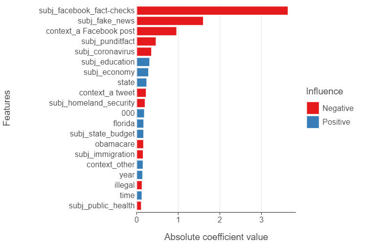
_ = lasso_classifier.fit(X_train, y_train)To peak “underneath the hood” of the Lasso model, we can explore which factors tend to predict truthful / untruthful statements. Unsurprisingly, subjects dealing with Facebook Fact-Checks and Fake News are the most indicative of untruthful statements. We see that topics such as education and the economy, however, are most indicative of truthful statements.
# Create a data frame of the top 20 features
top_20_feats = (
    pd.DataFrame({"features": lasso_classifier.feature_names_in_,
                  "coefs": lasso_classifier.coef_.reshape(-1)})
    .assign(abs_coefs = lambda x: np.abs(x["coefs"]),
            sign = lambda x: np.where(x["coefs"] > 0, "Positive", "Negative"))
    .sort_values("abs_coefs")
    .tail(20)
)

# Plot the output
(
    ggplot(top_20_feats, aes("abs_coefs", "features", fill = "sign")) +
    geom_bar(stat = "identity", tooltips=layer_tooltips().line("Abs. coef. value: @abs_coefs").line("@sign")) +
    theme(panel_grid_major_y=element_blank()) +
    labs(x = "Absolute coefficient value", y = "Features", fill = "Influence")
)
We can now apply our insights to the test set, to see how well our “optimal” model performs. We have an F1-score of 0.66, which is better than flipping a coin. Let’s see if we can get better performance using an XGBoost.
# Apply class predictions to the test set
predictions = lasso_classifier.predict(X_test)

# f1-score
np.round(f1_score(y_test, predictions), 2)

0.66
Supervised Learning: XGBoost
With XGBoost, we will vary the proportion of features sampled when building each tree in the model and the learning rate. To speed things up, we are going to take advantage of parallel processing by setting n_jobs = -1 which lets the algorithm run across
# Create a dictionary of hyperparameter values to try
xgb_params = {"n_estimators": [1000], "colsample_bytree":[0.3,0.6,0.9], "learning_rate": [0.001,0.01,0.1]}

# Instantiate an XGBoost classifier, utilising all cores in your laptop
xgb_classifier = XGBClassifier(n_jobs = -1)

# Create a 10-fold cross-validation algorithm
xgb_grid = GridSearchCV(xgb_classifier, param_grid=xgb_params, scoring="f1", cv=10)

# Fit the algorithm to the training data
_ = xgb_grid.fit(X_train, y_train)
We see that an XGBoost that uses 90% of features to build each decision tree and a learning rate of 0.01 produces the best results out of all the hyperparameter combinations we have tried.
xgb_grid.cv_results_["param_colsample_bytree"] = xgb_grid.cv_results_["param_colsample_bytree"].astype(str)

(
    ggplot(pd.DataFrame(xgb_grid.cv_results_), aes("param_learning_rate", "mean_test_score", color = "param_colsample_bytree")) +
    geom_point(tooltips=layer_tooltips().line("@mean_test_score")) +
    geom_line(linetype = "dashed") +
    theme(legend_position="bottom",
          panel_grid_major_x= element_blank()) +
    labs(x = "Learning rate", y = "Mean F-1 Score", color = "Proportion of features\nused in each tree",
         title = "An XGBoost that uses 90% of features and a learning rate of 0.01\nproduces the highest score!")
)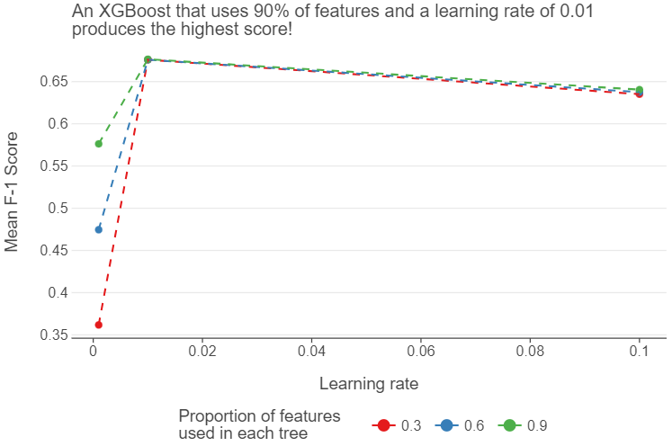
After having evaluated the data on the test set, we find that our F1-score improves by ~ 2 percentage points - noticeable, but there is still obviously room for improvement.
# Pick the best XGBoost
xgb_classifier = xgb_grid.best_estimator_

# Fit the best model to the training data
_ = xgb_classifier.fit(X_train, y_train)

# Apply class predictions to the test set
predictions = xgb_classifier.predict(X_test)

# f1-score
np.round(f1_score(y_test, predictions), 2)

0.68
Unsupervised learning approaches
In this part, we’ll extract insights from the LIAR datasets using a couple of different unsupervised techniques:
- clustering
- anomaly detection
- topic modeling
But, before we do that, we’ll pre-process the data again as the pre-processing here is a bit different from the pre-processing used in the supervised learning part (note that you could also have used the pre-processing performed here in the supervised learning part). The main reason for this pre-processing is to enhance the results of topic modeling (LDA performed on data pre-processed as in the supervised learning part doesn’t yield particularly meaningful results for this dataset!).
Pre-processing
texts = liar["statement"].astype(str).tolist()
def spacy_preprocess(texts):
    processed = []

    for doc in nlp.pipe(texts, batch_size=500):
        tokens = []

        for token in doc:
            if (
                token.is_punct or
                token.like_num or
                token.is_space or
                not token.is_alpha
            ):
                continue

            # Keep all named entities intact (e.g., "Affordable Care Act")
            if token.ent_type_ in {"PERSON", "ORG", "GPE", "LAW", "NORP", "EVENT"}:
                tokens.append(token.text.lower())
                continue

            # Keep only relevant parts of speech: NOUN, VERB, ADJ, ADV
            if token.pos_ in {"NOUN", "VERB", "ADJ", "ADV"}:
                lemma = token.lemma_.lower()
                tokens.append(lemma)

        processed.append(tokens)

    return processed

# Run preprocessor
tokenized_texts = spacy_preprocess(texts)

# Train bigram and trigram models
bigram_model = Phrases(tokenized_texts, min_count=3, threshold=5)
trigram_model = Phrases(bigram_model[tokenized_texts], threshold=5)

bigram_phraser = Phraser(bigram_model)
trigram_phraser = Phraser(trigram_model)

# Apply phrase detection
texts_bigrams = [bigram_phraser[doc] for doc in tokenized_texts]
texts_trigrams = [trigram_phraser[bigram_phraser[doc]] for doc in tokenized_texts]

# Final cleaned version
final_texts = [[w for w in doc if 2 < len(w) < 25] for doc in texts_trigrams]
The goal of the pre-processing is to clean and structure political statements for downstream analysis — without stripping away politically meaningful expressions like “tax cut”, “Donald Trump”, “Affordable Care Act”. Here’s what’s happening:
1️⃣ Step 1: Load LIAR data
texts = liar["statement"].astype(str).tolist()The dataset is loaded and converted to a list of strings (statement column).
2️⃣ Step 2 (within the spacy_preprocess function): spaCy Preprocessing Function
def spacy_preprocess(texts):
    processed = []

    for doc in nlp.pipe(texts, batch_size=500):
        tokens = []
for token in doc:- Batch processes texts using
spaCyfor speed. - Initializes a list of
tokensfor eachdoc(text).
3️⃣ Step 3 (within the spacy_preprocess function): Remove non-informative tokens
 if (
        token.is_punct or
        token.like_num or
        token.is_space or
        not token.is_alpha
    ):
        continue
Remove (i.e skip) punctuation, digits, whitespace, and anything that isn’t a proper word (is_alpha).
4️⃣ Step 4 (within the spacy_preprocess function): Preserve Named Entities (Important!)
if token.ent_type_ in {"PERSON", "ORG", "GPE", "LAW", "NORP", "EVENT"}:
    tokens.append(token.text.lower())
continue- If a token is part of a named entity (e.g., a law, person, organization, political event), we keep it as-is, lowercased.
- This ensures phrases like “Affordable Care Act” are preserved in the next step.
5️⃣ Step 5 (within the spacy_preprocess function): Filter POS tags (keep only meaningful words)
if token.pos_ in {"NOUN", "VERB", "ADJ", "ADV"}:
    lemma = token.lemma_.lower()
tokens.append(lemma)- Keeps only nouns, verbs, adjectives, and adverbs.
- Lemmatizes them (e.g., “running” → “run”, “better” → “good”).
6️⃣ Step 6: Generate Bigrams and Trigrams
bigram_model = Phrases(tokenized_texts, min_count=3, threshold=5)
trigram_model = Phrases(bigram_model[tokenized_texts], threshold=5)

bigram_phraser = Phraser(bigram_model)
trigram_phraser = Phraser(trigram_model)

texts_bigrams = [bigram_phraser[doc] for doc in tokenized_texts]
texts_trigrams = [trigram_phraser[bigram_phraser[doc]] for doc in tokenized_texts]- Learns common bigrams like
["tax", "cut"] → "tax_cut"and trigrams like["affordable", "care", "act"] → "affordable_care_act". threshold=5ensures only semi-frequent phrases are merged.
7️⃣ Step 7: Final Cleanup
final_texts = [[w for w in doc if 2 < len(w) < 25] for doc in texts_trigrams]Filters out tokens that are too short (like “a”, “it”) or too long (usually garbage).
Why is this pre-processing suitable for political text such as the LIAR dataset?
- We’re only removing punctuation, numbers, spaces, and non-alphabetic characters, while retaining important content.
- In particular, we keep named entities in their original form (just lowercased) rather than lemmatizing them, which maintains their recognizable identity. And we’ve included named entity types that are highly relevant in political discourse.
- We made a sensible part-of-speech selection. By including nouns, verbs, adjectives, and adverbs, we capture the key content words that convey meaning and sentiment in political statements.
- The addition of bigram and trigram detection is particularly valuable for political text, as it will capture important phrases like “health_care_reform” or “tax_policy” rather than treating the individual words separately.
- The final step of removing very short (≤2 character) and very long (≥25 character) tokens helps eliminate potential noise while keeping meaningful content.
This approach should preserve the important semantic content needed for analyzing political statements, including entities, topics, and sentiment-bearing words, while still providing useful normalization and noise reduction.
We’ll now construct a TF-IDF DFM.
docs = [" ".join(tokens) for tokens in final_texts]

# TF-IDF: preserve important phrases by analyzing words and bigrams
vectorizer = TfidfVectorizer(
    max_df=0.5,
    min_df=5,
    ngram_range=(1, 3),  # can also try (2, 3) for stricter phrase focus
)
X_tfidf = vectorizer.fit_transform(docs)
LSA for dimensionality reduction
We’ll use LSA to reduce dimensions before applying clustering or anomaly detection.
Let’s first start by choosing the number of components for LSA.
There are several methods to determine the number of components for LSA (some of which can also be used for LDA).
1. Explained Variance (LSA-specific)
| Method | Explained Variance (via TruncatedSVD) |
|---|---|
| Use Case | Latent Semantic Analysis (LSA) |
| Metric | Cumulative variance explained by components |
| How It Works | Selects the smallest number of components needed to explain a threshold (e.g., 90%) of variance in the TF-IDF matrix |
| Pros | Intuitive, quick to compute, gives a rough dimensionality estimate |
| Cons | May not reflect semantic coherence of topics, not meaningful for LDA or NMF |
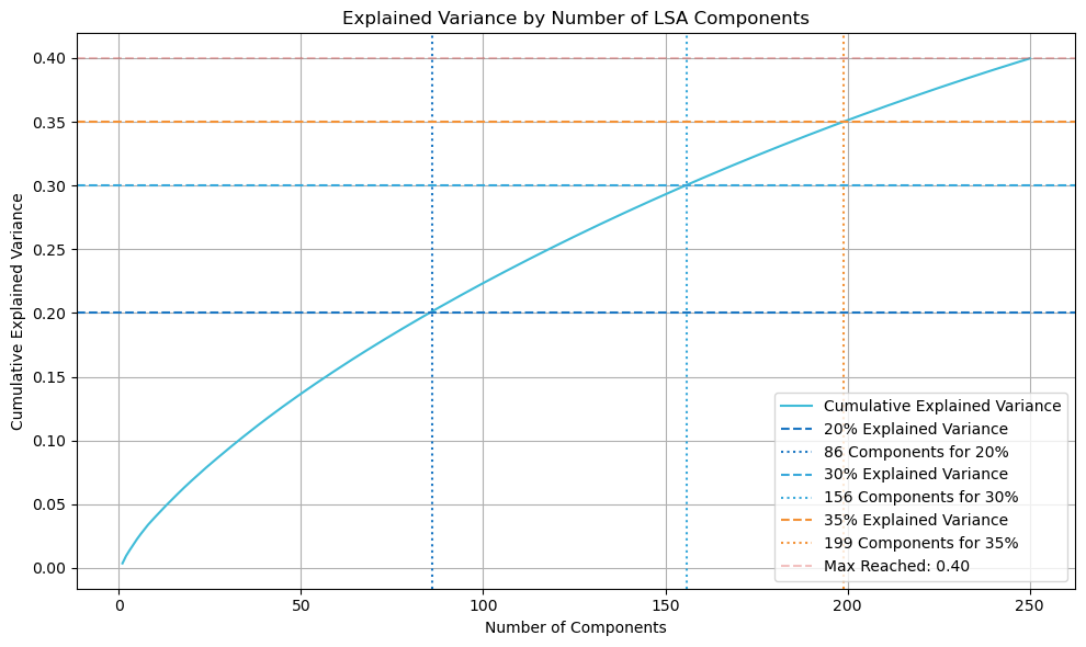
| Outcome in Our Case | No clear elbow or plateau was observed. Explained variance increased gradually without a strong inflection point. (see plot below) |
Click to view the code
def plot_explained_variance(X_tfidf, max_components=100, thresholds=[0.4, 0.5, 0.6, 0.7, 0.8]):
    """
    Plot cumulative explained variance from TruncatedSVD for LSA, and mark thresholds if they are reached.

    Returns a dictionary mapping thresholds to number of components needed (if reached).
    """
    n_components = min(max_components, X_tfidf.shape[1] - 1)
    svd = TruncatedSVD(n_components=n_components, random_state=42)
    svd.fit(X_tfidf)

    explained_variance = svd.explained_variance_ratio_
    cumulative_variance = np.cumsum(explained_variance)

    max_variance = cumulative_variance[-1]
    print(f"🔍 Max cumulative explained variance: {max_variance:.3f}")

    plt.figure(figsize=(10, 6))
    plt.plot(range(1, n_components + 1), cumulative_variance, color='#40BCD8', linestyle='-', label='Cumulative Explained Variance')
    plt.grid(True)
    plt.xlabel('Number of Components')
    plt.ylabel('Cumulative Explained Variance')
    plt.title('Explained Variance by Number of LSA Components')

    threshold_components = {}
    colors = ['#1C77C3', '#39A9DB', '#F39237', '#D63230', '#D63230']

    for i, threshold in enumerate(thresholds):
        if threshold <= max_variance:
            n_required = np.argmax(cumulative_variance >= threshold) + 1
            threshold_components[threshold] = n_required

            plt.axhline(y=threshold, color=colors[i % len(colors)], linestyle='--',
                        label=f'{int(threshold * 100)}% Explained Variance')
            plt.axvline(x=n_required, color=colors[i % len(colors)], linestyle=':',
                        label=f'{n_required} Components for {int(threshold * 100)}%')
        else:
            print(f"⚠️ Threshold {threshold} not reached (max = {max_variance:.2f})")

    # Optional: mark max variance level
    plt.axhline(y=max_variance, color='#D63230', linestyle='--', alpha=0.3,
                label=f'Max Reached: {max_variance:.2f}')

    plt.legend()
    plt.tight_layout()
    plt.show()

    return threshold_components
plot_explained_variance(X_tfidf, max_components=100, thresholds=[0.2,0.3,0.35]
2. AIC/BIC (Information Criteria)
| Method | AIC / BIC (Adapted from PCA-style residual reconstruction error) |
|---|---|
| Use Case | LSA (non-probabilistic) - adapted approach |
| Metric | Tradeoff between model fit (reconstruction error) and complexity |
| How It Works | Penalizes models with more parameters to avoid overfitting |
| Pros | Formal criterion for model selection |
| Cons | Not designed for SVD or non-generative models, results may be noisy/inconsistent in high-dimensional sparse text |
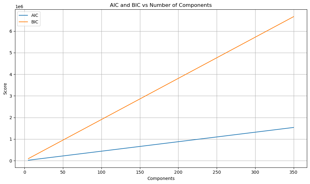
| Outcome in Our Case | No clear minima detected in AIC/BIC curves; insufficient for topic selection here (see plot below) |
Click to view the code
def compute_information_criteria(X_tfidf, component_range):
    n_samples, n_features = X_tfidf.shape
    aic_scores, bic_scores = [], []

    X_tfidf_dense = X_tfidf.toarray()

    for n_components in component_range:
        svd = TruncatedSVD(n_components=n_components, random_state=42)
        X_trans = svd.fit_transform(X_tfidf)
        X_approx = np.dot(X_trans, svd.components_)
        rss = np.sum((X_tfidf_dense - X_approx) ** 2)
        k = n_components * (n_features + 1)

        aic = n_samples * np.log(rss / n_samples) + 2 * k
        bic = n_samples * np.log(rss / n_samples) + k * np.log(n_samples)

        aic_scores.append(aic)
        bic_scores.append(bic)

    plt.figure(figsize=(10, 6))
    plt.plot(component_range, aic_scores, label='AIC')
    plt.plot(component_range, bic_scores, label='BIC')
    plt.xlabel('Components')
    plt.ylabel('Score')
    plt.title('AIC and BIC vs Number of Components')
    plt.legend()
    plt.grid(True)
    plt.tight_layout()
    plt.show()

    best_aic = component_range[np.argmin(aic_scores)]
    best_bic = component_range[np.argmin(bic_scores)]

    return best_aic, best_bic

compute_information_criteria(X_tfidf,component_range)
3. Topic Stability (LSA/LDA/NMF-compatible)
| Method | Topic Stability (Jaccard similarity across runs) |
|---|---|
| Use Case | Any model where randomness influences output |
| Metric | Average pairwise similarity of top terms per topic across multiple model runs |
| Pros | Robust, directly measures semantic consistency |
| Cons | Requires multiple model fits; computationally more expensive |
| Outcome in Our Case | This metric shows a sharp decline until about [50] components then stabilizes with a slight uptick after 150 components (see outcome of code chunk below) |
4. Topic Quality (Diversity & Exclusivity)
| Method | Topic Quality Metrics |
|---|---|
| Use Case | Any topic model |
| Metrics | Diversity: unique words across topics; Exclusivity: words unique to single topics |
| Pros | Directly measures topic interpretability and separability |
| Cons | Somewhat heuristic, though intuitive and easy to interpret |
| Outcome in Our Case | Clear “elbow” observed between [50-75] components for both diversity and exclusivity, indicating high-quality topics (see outcome of code chunk below) |
We’ll use topic stability and topic quality (i.e exclusivity+diversity) to select the number of LSA component in this particular case.
Why topic stability + topic quality?
In our case, traditional quantitative metrics like explained variance and AIC/BIC did not yield clear-cut or meaningful selection criteria. Instead, we observed visually and quantitatively well-defined optima (see the results of the code chunk below) using:
- Topic Stability: A strong indicator of model consistency across different initializations.
- Topic Quality (Diversity + Exclusivity): Highlighted a point where topics are both distinct and interpretable.
This dual-criterion approach is particularly well-suited to exploratory or unsupervised text analysis, where interpretability and robustness matter more than pure statistical fit.
Higher stability (Jaccard similarity) indicates more consistent topics across different runs, while quality metrics tell you how interpretable those topics are. When selecting the optimal number of components for LSA, we’re looking for:
- Stability (Jaccard similarity) as high as possible - indicating that our topic assignments are consistent across different runs rather than randomly changing.
- Quality metrics (Diversity and Exclusivity) that have reached an elbow point - where adding more components gives diminishing returns.
In our graphs (see results of code chunk below), around 50-75 components seems to be where both conditions start to be met. After this point:
- Stability levels off and even slightly improves
- Quality metrics stop their steep decline and flatten out
This “elbow point” represents a sweet spot where we have enough components to capture meaningful patterns in our data, but not so many that we’re just modeling noise or creating unstable, overlapping topics. A lower component count (e.g 10) might give higher absolute stability scores but at the cost of poor quality metrics, while very high component counts don’t meaningfully improve any of the metrics.
We choose 70 here.
fine_grained_range = list(range(1, 51))+list(range(60, 201, 10)) #iteration range (step of 1 from 1 to 50 and step of 10 between 50 and 200).

# Extract topics from SVD
def get_topics_from_svd(svd_model, feature_names, n_top_words=10):
    word_indices = np.argsort(svd_model.components_, axis=1)[:, -n_top_words:]
    return np.array(feature_names)[word_indices][:, ::-1]

# 1. Topic Stability
def evaluate_stability(X_tfidf, feature_names, component_range, n_runs=5, n_top_words=10):
    stability_scores = []
    for n_components in component_range:
        runs_topics = []
        for seed in range(n_runs):
            svd = TruncatedSVD(n_components=n_components, random_state=seed)
            svd.fit(X_tfidf)
            topics = get_topics_from_svd(svd, feature_names, n_top_words)
            runs_topics.append(topics)

        sim_scores = []
        for i in range(n_runs):
            for j in range(i + 1, n_runs):
                sim = [
                    len(set(t1) & set(t2)) / len(set(t1) | set(t2))
                    for t1, t2 in zip(runs_topics[i], runs_topics[j])
                ]
                sim_scores.append(np.mean(sim))
        stability_scores.append(np.mean(sim_scores))

    plt.figure(figsize=(10, 6))
    plt.plot(component_range, stability_scores, 'm-o')
    plt.xlabel('Components')
    plt.ylabel('Avg Jaccard Similarity')
    plt.title('Topic Stability Across Runs')
    plt.grid(True)
    plt.tight_layout()
    plt.show()

    return stability_scores

# 2. Topic Quality
def calculate_topic_metrics(X_tfidf, feature_names, component_range, n_top_words=10):
    diversity_scores, exclusivity_scores = [], []

    for n_components in component_range:
        svd = TruncatedSVD(n_components=n_components, random_state=42)
        svd.fit(X_tfidf)
        topics = get_topics_from_svd(svd, feature_names, n_top_words)

        all_words = [word for topic in topics for word in topic]
        diversity = len(set(all_words)) / len(all_words)

        counts = Counter(all_words)
        exclusivity = sum(1 for v in counts.values() if v == 1) / len(counts)

        diversity_scores.append(diversity)
        exclusivity_scores.append(exclusivity)

    plt.figure(figsize=(10, 6))
    plt.plot(component_range, diversity_scores, label='Diversity', color='blue')
    plt.plot(component_range, exclusivity_scores, label='Exclusivity', color='red')
    plt.xlabel('Components')
    plt.ylabel('Score')
    plt.title('Topic Quality Metrics')
    plt.legend()
    plt.grid(True)
    plt.tight_layout()
    plt.show()

    return diversity_scores, exclusivity_scores

# 3. Component Analysis function
def analyze_components(X_tfidf, final_texts, vectorizer, component_range):
    feature_names = vectorizer.get_feature_names_out()
    dictionary = Dictionary(final_texts)

    print("\n1. Evaluating Topic Stability...")
    stability_scores = evaluate_stability(X_tfidf, feature_names, component_range)

    print("\n2. Evaluating Topic Quality...")
    diversity_scores, exclusivity_scores = calculate_topic_metrics(X_tfidf, feature_names, component_range)

    print("\n=== Analysis Complete ===")
    print("Based on the plots, manually set the optimal number of components.")

    return None

# Run the analysis to generate plots
analyze_components(X_tfidf, final_texts, vectorizer, fine_grained_range)

# After viewing the plots, set your chosen number of components here:
selected_components = 70  # Change this value based on your analysis of the plots

print(f"\nSelected number of components: {selected_components}")
1. Evaluating Topic Stability...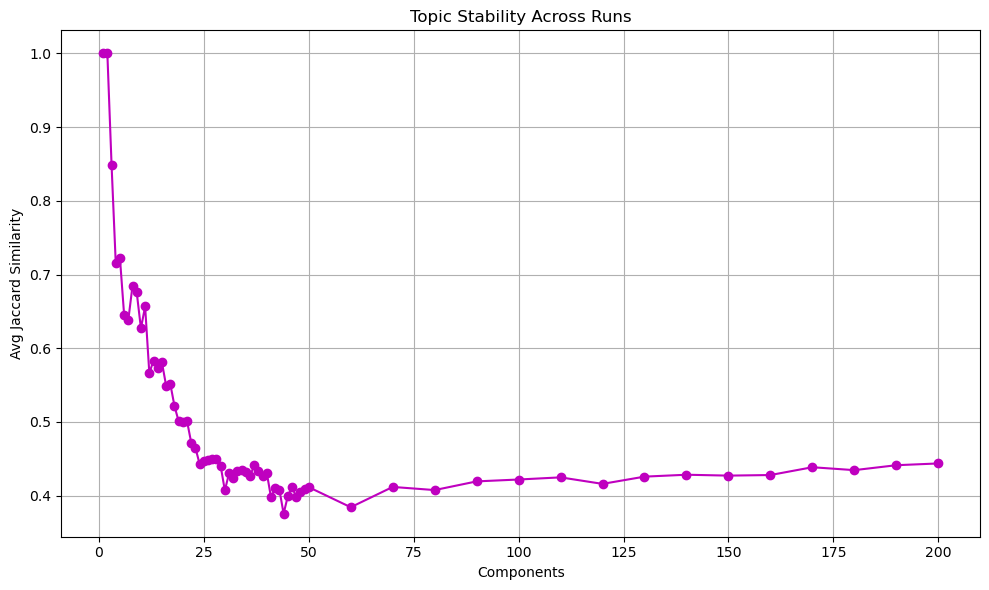
2. Evaluating Topic Quality...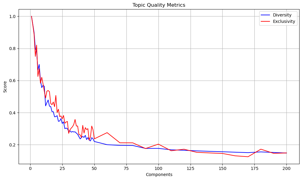
=== Analysis Complete ===
Based on the plots, manually set the optimal number of components.

Selected number of components: 70
After the number of components (“topics”) have been selected, we’re ready to run LSA.
svd = TruncatedSVD(n_components=selected_components, random_state=42)
X_lsa = svd.fit_transform(X_tfidf)
lsa_cols = [f'lsa_{i}' for i in range(selected_components)]  # lsa_0, lsa_1, ..., lsa_n-1
X_lsa_df = pd.DataFrame(X_lsa, columns=lsa_cols)
Clustering
For this part, we’ll combine both the matrix obtained with LSA and metadata from the original liar dataframe (the one-hot encoded subject columns i.e the columns prefixed with subj_, the column with information about the speaker i.e speaker, the date column i.e date and the column that contains information about how true the statement is i.e perc_true).
Before we proceed, let’s have a quick look at missing values in the metadata.
selected_columns = ['speaker', 'date', 'perc_true']

# Dynamically add all columns starting with 'subj_'
subj_columns = [col for col in liar.columns if col.startswith('subj_')]

# Combine the initial selection with the dynamically selected columns
final_columns = selected_columns + subj_columns
missing_counts = liar[final_columns].isna().sum()

# Convert to DataFrame for better visualization
missing_summary = missing_counts.reset_index()
missing_summary.columns = ['Column', 'Missing Values']
missing_summary| Column | Missing Values | |
|---|---|---|
| 0 | speaker | 7 |
| 1 | date | 7 |
| 2 | perc_true | 0 |
| 3 | subj_government_regulation | 0 |
| 4 | subj_polls_and_public_opinion | 0 |
| … | … | … |
| 177 | subj_katrina | 0 |
| 178 | subj_ohio | 0 |
| 179 | subj_nbc | 0 |
| 180 | subj_georgia | 0 |
| 181 | subj_missouri | 0 |
182 rows × 2 columns
There are a few missing values for speaker and date (and not obvious way to impute them). So we’ll just drop those rows before we proceed with clustering.
# Identify valid (non-missing) rows based on speaker and date
valid_rows = liar["speaker"].notna() & liar["date"].notna()

# Filter liar and X_lsa accordingly
liar_clean = liar[valid_rows].copy()
liar_clean.reset_index(drop=True, inplace=True)
We drop the rows from the LSA matrix that correspond to missing values of speaker and date.
X_lsa_clean_df = X_lsa_df[valid_rows].copy()

# Reset the index for consistency
X_lsa_clean_df.reset_index(drop=True, inplace=True)
Now, we’re ready to pre-process the metadata before going on with clustering:
- the
subj_columns are already one-hot encoded and don’t require further pre-processing - similarly,
perc_trueis already scaled (it’s in a scale between 0-1) and doesn’t require further pre-processing - for speakers, we only keep the top 20 speakers and replace the values of the others by “Other” (this prevents having data that is too sparse) before one-hot encoding the
speakercolumn - for the
datecolumn, we only keep the year, bin years into discrete intervals (e.g., 1999-2005, 2005-2010, etc.) then encode these intervals as numerical labels for modeling
# 1. Use subj_ columns as-is
subj_cols = liar_clean.filter(regex=r'^subj_').columns
X_subj = liar_clean[subj_cols]  # already binary, no processing needed

# 2. Use perc_true as-is
X_truth = liar_clean[["perc_true"]]

# 3. Process speaker — limit to top N, encode rest as "Other", then one-hot
top_speakers = liar_clean["speaker"].value_counts().nlargest(20).index
liar_clean["speaker_grouped"] = liar_clean["speaker"].where(liar_clean["speaker"].isin(top_speakers), "Other")

speaker_encoder = OneHotEncoder(sparse_output=False, handle_unknown='ignore')
speaker_encoded = speaker_encoder.fit_transform(liar_clean[["speaker_grouped"]])
speaker_cols = speaker_encoder.get_feature_names_out(["speaker_grouped"])
df_speaker = pd.DataFrame(speaker_encoded, columns=speaker_cols, index=liar_clean.index).astype(int)

# 4. Process date — bin by year
liar_clean["year"] = pd.to_datetime(liar_clean["date"]).dt.year
df_year = pd.cut(liar_clean["year"], bins=[1999, 2005, 2010, 2015, 2020, 2025], labels=False)
df_year = pd.DataFrame({"year_encoded": df_year.astype(int)}, index=liar_clean.index)

df_meta = pd.concat([X_subj, X_truth, df_speaker, df_year], axis=1)
meta_cols = df_meta.columns.tolist()
We’re now ready for clustering. Since we are combining both numeric and categorical features in our input matrix, our metric of choice is the Gower distance/similarity, which supports mixed data types. This rules out some standard algorithms:
- KMeans is incompatible because it assumes Euclidean space and doesn’t handle categorical features.
- DBSCAN works with Gower but fails on this dataset due to variable densities — we tested it but omit the results for clarity (the same is true for other density-based techniques that extend DBSCAN such as HDBSCAN and OPTICS: our tests, also not shown for concision, reveal the same pattern as with DBSCAN i.e clustering the whole data into a single cluster).
Instead, we explore three algorithms: - KMedoids, which is robust and Gower-compatible
- Spectral Clustering, ideal for complex structures
- Fuzzy C-Means, a soft clustering method that offers probabilistic assignments
🧩 KMedoids
KMedoids is a partitioning-based clustering method related to KMeans, but it selects actual data points (medoids) as cluster centers rather than computing means. This makes it more interpretable and robust to noise, especially when using arbitrary distance metrics like Gower.
How it works:
- Initialize
kmedoids randomly - Assign each point to the nearest medoid using Gower distance
- Swap medoids to minimize overall intra-cluster dissimilarity
- Repeat until convergence
| Feature | KMeans | KMedoids |
|---|---|---|
| Cluster center | Mean | Actual data point (medoid) |
| Distance metric | Euclidean | Any (e.g., Gower) |
| Noise sensitivity | High | Lower |
| Mixed data support | ❌ | ✅ (with Gower) |
| Interpretability | Lower | Higher |
✅ Pros & ❌ Cons
| Pros | Cons |
|---|---|
| Works with arbitrary distances (e.g., Gower) | Slower than KMeans on large datasets |
| More robust to noise and outliers | Still requires k to be known |
| Medoids are real data points (interpretable) | Less scalable than centroid-based methods |
🌈 Spectral Clustering
Spectral Clustering is a graph-based method that uses the eigenstructure of a similarity matrix to uncover clusters. It excels in detecting non-convex, manifold-shaped, or globally-connected clusters — useful in complex datasets combining text and metadata.
How it works:
- Convert Gower distances to similarities (e.g.,
1 - Gower) - Build a graph Laplacian from the similarity matrix
- Compute eigenvectors (spectral embedding)
- Apply clustering (typically KMeans) in the embedded space
| Feature | Spectral Clustering | KMedoids |
|---|---|---|
| Graph-based? | ✅ | ❌ |
Requires k? |
✅ | ✅ |
| Handles mixed data? | ✅ (via Gower similarity) | ✅ (via Gower distance) |
| Works with complex shapes? | ✅ | Moderate |
✅ Pros & ❌ Cons
| Pros | Cons |
|---|---|
| Captures global data structure | Requires precomputed similarity matrix |
| Ideal for complex, non-linear cluster shapes | Memory-intensive on large datasets |
| Supports Gower-derived similarity | Requires number of clusters (k) |
| Good for clustering on text + metadata | Sensitive to scale in similarity values |
🌫️ Fuzzy C-Means
Fuzzy C-Means (FCM) is a soft clustering algorithm that assigns partial membership to clusters — useful when cluster boundaries are ambiguous, as with political statements or nuanced text.
⚠️ Limitation: FCM requires Euclidean distance, so we must convert all features to numeric, typically through one-hot encoding for categoricals. This allows the algorithm to run but slightly changes the nature of the data.
How it works:
- Initialize cluster centers
- Compute fuzzy membership scores for each point
- Update cluster centers using weighted averages
- Repeat until convergence
✅ Pros & ❌ Cons
| Pros | Cons |
|---|---|
| Captures ambiguity and overlapping clusters | Requires numeric-only input (not compatible with Gower) |
| Soft assignments give richer interpretation | Sensitive to outliers and initialization |
| Useful when clusters are not crisply defined | Assumes Euclidean space → categorical encoding may distort data |
🧮 Clustering Comparison
| Feature | KMedoids / Spectral | Fuzzy C-Means |
|---|---|---|
| Assignment type | Hard (1 cluster per point) | Soft (multiple memberships per point) |
| Input requirement | Precomputed distances (e.g., Gower for mixed data) | Numeric matrix (e.g., one-hot encoded categoricals) |
| Distance metric | Arbitrary (via Gower) | Euclidean (assumes numeric structure) |
| Handles ambiguity? | ❌ | ✅ |
| Works with Gower? | ✅ (direct Gower compatibility) | ❌ (not directly — requires transformation) |
| Handles mixed data? | ✅ (via Gower) | ⚠️ Indirectly — requires numeric encoding |
⚠️ Note: While Fuzzy C-Means doesn’t natively handle categorical variables, it can be applied after transforming mixed data into a fully numeric matrix (e.g., via one-hot encoding). However, doing so introduces Euclidean assumptions that may not reflect true semantic distances, especially with sparse features.
# Function to sanitize text for plotting
def sanitize_text(statement, max_length=100):
    sanitized = statement.replace('$', r'\$').replace('"', r'\"').replace("'", r"\'")
    return sanitized[:max_length] + '...' if len(sanitized) > max_length else sanitized

df_combined = pd.concat([X_lsa_clean_df.reset_index(drop=True), df_meta.reset_index(drop=True)], axis=1)

# --- Set correct dtypes ---

# subj_ columns: binary categorical → set to object for Gower to detect them
for col in subj_cols:
    df_combined[col] = df_combined[col].astype("object")

# perc_true: numeric
df_combined["perc_true"] = df_combined["perc_true"].astype(float)

# speaker columns (already one-hot encoded): also binary categorical
for col in df_speaker.columns:
    df_combined[col] = df_combined[col].astype("object")

# year_encoded: ordinal categorical
df_combined["year_encoded"] = df_combined["year_encoded"].astype("object")
We need to determine the number of clusters for Spectral Clustering, KMedoid, and Fuzzy C-Means. For Spectral and KMedoid, we use the Dunn Index. For Fuzzy C-Means, which produces soft cluster memberships, we use the Xie-Beni Index, a metric specifically designed for fuzzy clustering.
The Dunn Index is more robust than the Silhouette score when working with Gower distance for mixed data types. While both metrics can technically work with precomputed distance matrices, the Dunn Index’s focus on cluster separation rather than compactness makes it better suited for the non-Euclidean nature of Gower distances. Other metrics like Calinski-Harabasz and Davies-Bouldin require Euclidean spaces and cannot be directly applied to Gower distances without transformation.
📊 Dunn Index
What is it?
The Dunn Index is an internal clustering validation metric defined as:
Dunn Index = (Minimum inter-cluster distance) / (Maximum intra-cluster distance)
- Encourages tight, well-separated clusters
- Used across different
kvalues to select the best clustering
Use in Practice
- Higher Dunn Index = better clustering
- Used to choose
kfor Spectral Clustering and KMedoids
| Aspect | Value |
|---|---|
| Best when | Inter-cluster distance is high, intra-cluster tight |
| Output range | ≥ 0 (higher is better) |
| Pros | Simple, interpretable |
| Cons | Sensitive to noise |
🌀 Xie-Beni Index
What is it?
The Xie-Beni Index is a validity metric tailored to fuzzy clustering (like Fuzzy C-Means). It considers both fuzzy membership strength and cluster separation, offering a balance between compactness and separation in soft clustering contexts.
Xie-Beni Index = (Total weighted intra-cluster variance) / (Minimum cluster center distance²)
Why not Dunn or other indices?
Unlike Spectral or KMedoid, Fuzzy C-Means doesn’t assign each point to a single cluster. Instead, each point has degrees of membership across all clusters. Traditional validation metrics like Dunn, Silhouette, Calinski-Harabasz, or Davies-Bouldin are designed for hard (crisp) clustering, where every point belongs to exactly one cluster. Applying these to fuzzy results would require forced binarization (e.g. via argmax), which discards the soft nature of the clustering and leads to misleading evaluations.
The Xie-Beni Index, by contrast:
- Accounts for soft assignments directly (using membership weights)
- Evaluates the balance between compactness and separation in the fuzzy space
- Naturally penalizes overlapping clusters and under-separation
Use in Practice
- Lower Xie-Beni Index = better clustering
- Used to choose
c(number of clusters) for Fuzzy C-Means
| Aspect | Value |
|---|---|
| Best when | Clusters are compact and well-separated with low overlap |
| Output range | ≥ 0 (lower is better) |
| Pros | Designed for fuzzy clustering, interprets soft labels |
| Cons | Sensitive to outliers and high-dimensional noise |
def dunn_index(distance_matrix, labels):
    unique_clusters = np.unique(labels)

    intra_dists = []
    for i in unique_clusters:
        cluster_indices = np.where(labels == i)[0]
        if len(cluster_indices) > 1:
            intra_cluster_dist = np.max(distance_matrix[np.ix_(cluster_indices, cluster_indices)])
        else:
            intra_cluster_dist = 0
        intra_dists.append(intra_cluster_dist)

    inter_dists = []
    for i in unique_clusters:
        for j in unique_clusters:
            if i < j:
                idx_i = np.where(labels == i)[0]
                idx_j = np.where(labels == j)[0]
                if len(idx_i) > 0 and len(idx_j) > 0:
                    inter_cluster_dist = np.min(distance_matrix[np.ix_(idx_i, idx_j)])
                    inter_dists.append(inter_cluster_dist)

    if not intra_dists or not inter_dists or np.max(intra_dists) == 0:
        return np.nan

    return np.min(inter_dists) / np.max(intra_dists)

def dunn_evaluation(distance_matrix, mode="kmedoids", values=None):
    scores = []
    labels_all = []

    if values is None:
        values = range(2, 11)

    for v in tqdm(values, desc=f"Dunn Index ({mode})"):
        try:
            match mode:
                case "kmedoids":
                    model = KMedoids(n_clusters=v, metric='precomputed', random_state=42)
                    model.fit(distance_matrix)
                    labels = model.labels_

                case "spectral":
                    sim = 1 - distance_matrix
                    model = SpectralClustering(n_clusters=v, affinity='precomputed', random_state=42).fit(sim)
                    labels = model.labels_

                case _:
                    raise ValueError(f"Unsupported mode: {mode}")

            score = dunn_index(distance_matrix, labels)
            scores.append(score)
            labels_all.append(labels)

        except Exception as e:
            print(f"{mode} {v} failed: {e}")
            scores.append(np.nan)
            labels_all.append(None)

    return values, scores, labels_all


def plot_index(values, scores, title, x_label="k",index="Dunn"):
    df = pd.DataFrame({'value': values, 'dunn': scores}).dropna()
    return (
        ggplot(df, aes(x='value', y='dunn')) +
        geom_line(color='#1C77C3') +
        geom_point(color='#1C77C3', size=3) +
        ggtitle(title) +
        xlab(x_label) + ylab(index+" Index") +
        theme_minimal()
    )

def xie_beni_index(X, u, centers, m=2):
    n_clusters = centers.shape[0]
    N = X.shape[0]

    um = u ** m
    dist = np.zeros((n_clusters, N))
    for k in range(n_clusters):
        dist[k] = np.linalg.norm(X - centers[k], axis=1) ** 2

    compactness = np.sum(um * dist)

    min_dist = np.min([
        np.linalg.norm(centers[i] - centers[j]) ** 2
        for i in range(n_clusters) for j in range(n_clusters) if i != j
    ])
    return compactness / (N * min_dist)

def xie_beni_evaluation(X, values=range(2, 11)):

    scores = []
    labels_all = []

    for c in tqdm(values, desc="Xie-Beni Index (Fuzzy C-Means)"):
        try:
            cntr, u, _, _, _, _, _ = cmeans(
                X.T, c, m=2.0, error=0.005, maxiter=1000, init=None
            )
            xb = xie_beni_index(X, u, cntr)
            scores.append(xb)
            labels_all.append(np.argmax(u, axis=0))  # hard labels
        except Exception as e:
            print(f"Fuzzy c={c} failed: {e}")
            scores.append(np.nan)
            labels_all.append(None)

    return values, scores, labels_all


#Computing the Gower distance matrix
gower_dist = gower_matrix(df_combined)

# KMedoids
ks_k, dunn_k, labels_k = dunn_evaluation(gower_dist, mode="kmedoids", values=range(2, 11))
plot_kmedoid = plot_index(ks_k, dunn_k, title="Dunn Index — KMedoids", x_label="k",index="Dunn")

# Spectral
ks_s, dunn_s, labels_s = dunn_evaluation(gower_dist, mode="spectral", values=range(2, 11))
plot_spectral = plot_index(ks_s, dunn_s, title="Dunn Index — Spectral Clustering", x_label="k",index="Dunn")

# Fuzzy

fuzzy_input = df_combined.copy()

for col in fuzzy_input.columns:
    if fuzzy_input[col].dtype == 'object':
        # Try to convert to numeric
        try:
            fuzzy_input[col] = pd.to_numeric(fuzzy_input[col], errors='raise')
        except:
            # If that fails, use factorize (for true categorical text)
            fuzzy_input[col] = pd.factorize(fuzzy_input[col])[0]

# At this point, all columns should be numeric
fuzzy_input = fuzzy_input.fillna(0).astype(np.float64)
X_fuzzy = fuzzy_input.values
c_means_input = X_fuzzy.T
ks_f, xie_beni_f, labels_f = xie_beni_evaluation(c_means_input, values=range(2, 11))
plot_fuzzy = plot_index(ks_f, xie_beni_f, title="Xie-Beni Index — Fuzzy C-Means Clustering", x_label="c",index="Xie-Beni")
Dunn Index (kmedoids): 100%|██████████| 9/9 [00:04<00:00, 2.06it/s]
Dunn Index (spectral): 100%|██████████| 9/9 [00:45<00:00, 5.09s/it]
Xie-Beni Index (Fuzzy C-Means): 100%|██████████| 9/9 [00:04<00:00, 2.09it/s]g=gggrid([
plot_kmedoid,
plot_spectral,
plot_fuzzy
], ncol=3)
g+=ggsize(1400,800)
g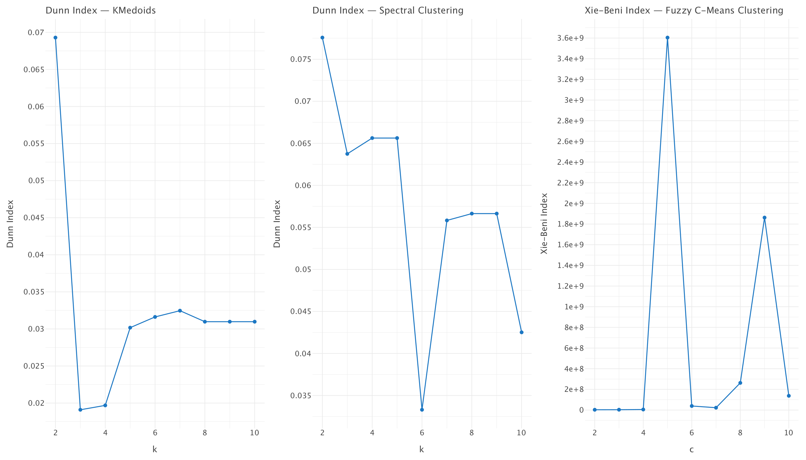
Looking at these plots, each clustering method shows different patterns for determining the optimal number of clusters:
KMedoids (Dunn Index): Shows the highest value at k=2, then drops significantly and gradually increases until k=6 before flattening. While k=2 has the highest Dunn Index, this could be creating overly broad clusters. The “elbow” appears around k=5, which might represent a better balance between cluster separation and meaningful groupings.
Spectral Clustering (Dunn Index): Shows the highest value at k=2, with another peak at k=4-5, then a drop at k=6, followed by another stable period at k=7-9. The interesting feature here is the local maximum at k=4-5, suggesting these might be meaningful cluster counts.
Fuzzy C-Means (Xie-Beni Index): For Xie-Beni Index, lower values indicate better clustering. There’s a significant spike at c=5, which should be avoided. The lowest values appear at c=2,c=3 and c=7, with c=2-3 showing the absolute minimum.
To select the optimal number of clusters, we should compare across methods and look for agreement between methods. \(K=7\) appears to be reasonable across all three plots (rising in KMedoids, local peak in Spectral, local minimum in Fuzzy C-Means).
Given the evidence from these plots, k=7 appears to be a reasonable choice that’s supported across methods while avoiding the extreme values that might represent either too few or too many clusters.
# Try a fixed number of clusters
gower_sim = 1-gower_dist
n_clusters = 7

# --- Spectral Clustering ---
spec_7clusters = SpectralClustering(n_clusters=n_clusters, affinity='precomputed', random_state=42)
labels_spec_7clusters = spec_7clusters.fit_predict(gower_sim)

kmedoids_7clusters = KMedoids(n_clusters=n_clusters, metric='precomputed',random_state=42,max_iter=300)

# Fit the model
kmedoids_7clusters.fit(gower_dist)
# Get cluster labels
labels_7clusters = kmedoids_7clusters.labels_

# Run Fuzzy C-means
cntr_7clust, u_7clust, _, _, _, _, _ = cmeans(
    c_means_input, c=n_clusters, m=2.0, error=0.005, maxiter=1000, init=None
)

labels_fuzzy_7clust = np.argmax(u_7clust, axis=0)
Since our clustering is performed on the high dimensional matrix directly (5733 by 5733 Gower distance matrix for Spectral clustering and KMedoid and original 5733 by 272 matrix for Fuzzy C-means!), we need to reduce the dimensionality of our data with UMAP to be able to visualise it.
umap_model_2d = umap.UMAP(n_components=2, metric='precomputed', random_state=42)
umap_embedding_2d = umap_model_2d.fit_transform(gower_dist)
umap_model_fuzzy = umap.UMAP(n_components=2, metric='euclidean', random_state=42)
umap_embedding_fuzzy = umap_model_fuzzy.fit_transform(X_fuzzy)

# Plotting helper
def plot_clusters(xy, labels, title, meta):
    df_plot = pd.DataFrame({
        "x": xy[:, 0],
        "y": xy[:, 1],
        "cluster": labels.astype(str),  # 👈 Cast to string
        "statement": meta["statement"],
        "perc_true": meta["perc_true"],
        "speaker": meta["speaker"],
        "date": meta["date"]
    })

    fig = px.scatter(df_plot, x='x', y='y', color='cluster',
                     hover_data=["statement", "perc_true", "speaker", "date"],
                     opacity=0.7, title=title,
                     color_discrete_sequence=px.colors.qualitative.T10)  # optional: better color palette
    fig.show()

X_combined_index = liar_clean.index

# Plot Spectral
plot_clusters(umap_embedding_2d, labels_spec_7clusters, "Spectral Clustering (n=7)", liar_clean.loc[X_combined_index])

# Plot KMedoid
plot_clusters(umap_embedding_2d, labels_7clusters, "KMedoid Clustering (n=7)", liar_clean.loc[X_combined_index])

plot_clusters(umap_embedding_fuzzy, labels_fuzzy_7clust, "Fuzzy C-Means Clustering (n=7)", liar_clean.loc[X_combined_index])
What does this clustering tell us?
Looking at our clustering results with n=7 across the three different methods (Fuzzy C-Means, KMedoid, and Spectral Clustering), alongside differences in data preprocessing, we can draw several important insights regarding our dataset’s underlying structure and the suitability of this cluster count.
Fuzzy C-Means Clustering (n=7 on raw mixed data)
Despite specifying 7 clusters, the visualization reveals only two distinct clusters (labeled 3 and 4), with cluster 4 showing some internal structure. This outcome suggests:
- The algorithm has effectively collapsed the data into a binary structure, assigning almost all points to just two major groups.
- This may indicate that our original feature space contains a dominant binary signal, possibly due to a few influential features.
- Membership values are largely concentrated, which implies that the fuzzy clustering doesn’t detect 7 meaningful divisions in this raw representation.
This aligns with our validation metrics (Dunn Index and Xie-Beni), both of which also pointed to 2–3 clusters as potentially optimal.
KMedoid Clustering (n=7 on Gower distance matrix)
This method produced well-separated clusters across the 2D UMAP projection, with all 7 clusters (0–6) clearly represented:
- Some clusters (e.g., 0, 1, 2) are distinctly separated, particularly on the left side of the visualization.
- Others (3, 4, 6) show more overlap in the center-right region, suggesting either fuzzier boundaries or latent substructure.
- Clusters generally appear coherent and well-shaped, indicating meaningful groupings in the transformed space.
Using the Gower distance matrix here proves advantageous, as it allows for balanced handling of both categorical and numeric features in your dataset.
Spectral Clustering (n=7 on Gower distance matrix)
Spectral clustering yielded a similar structure to KMedoid, supporting the validity of the Gower representation:
- All 7 clusters are visible, with cluster 3 forming a distinct band.
- While the overall shapes differ slightly from KMedoid (especially in the right half), the core structural patterns are consistent.
- There is some overlap between clusters, but also clear regions of separation, especially on the left.
Comparison Across Methods
- Consistency:
- KMedoid and Spectral clustering show similar global patterns, validating the structure uncovered via the Gower matrix.
- Fuzzy C-Means deviates significantly, emphasizing a binary grouping — this difference stems from working directly on the raw feature space.
- Data Representation Matters:
- Fuzzy C-Means is sensitive to dominant features in the raw data and may be overpowered by a few strong signals.
- The Gower distance matrix enables more nuanced group detection by normalizing contributions across mixed feature types.
- Cluster Separability and Interpretability:
- Fuzzy C-Means suggests a high-level binary division might be most natural.
- KMedoid and Spectral offer finer-grained subgroups, useful for in-depth exploration or downstream tasks like classification or profiling.
Conclusions
- If our goal is high-level categorization (e.g., separating broad truth/falsity groupings or political leanings):
- Fuzzy C-Means with 2–3 clusters might be optimal.
- If our goal is detailed segmentation of our dataset that respects the complex interplay of text and metadata:
- KMedoid or Spectral clustering with n=7, using the Gower matrix, provides better differentiation and structure.
Digging a bit further into Fuzzy C-Means
A peculiarity of Fuzzy C-Means is that it doesn’t quite assign a definitive cluster label to each data point. Instead, it produces a membership matrix \(U\), where each entry \(u_{ij}\) indicates the degree to which point \(j\) belongs to cluster \(i\). These degrees sum to 1 across clusters for each point, reflecting a soft assignment.
The typical practice of assigning each data point to a single cluster is done a posteriori by selecting the cluster with the highest membership score — mathematically, by taking the argmax over the membership matrix. This effectively converts the soft assignment into a hard label, creating a crisp partition similar to what you’d get from KMeans or KMedoids. While this makes comparison across clustering methods easier, it discards the soft assignment information — and in doing so, may obscure meaningful ambiguity or uncertainty in the data.
One way to better understand this ambiguity is to visualize the maximum membership strength each point has. A value near 1 indicates a confident assignment, while lower values suggest that the point lies closer to a boundary between clusters, or shares affinities with multiple groupings.
Below is a UMAP projection of the data used in the fuzzy clustering step, where points are colored by their maximum membership value:
# Max membership value per point (degree of "confidence")
max_membership = u_7clust.max(axis=0)

# Create a DataFrame for plotting
df_membership_plot = pd.DataFrame({
    "x": umap_embedding_fuzzy[:, 0],
    "y": umap_embedding_fuzzy[:, 1],
    "max_membership": max_membership
})

# Plot: color by maximum membership value
fig = px.scatter(df_membership_plot, x='x', y='y',
                 color='max_membership',
                 color_continuous_scale='viridis',
                 title="Fuzzy C-Means: Maximum Membership Strength (UMAP projection)",
                 opacity=0.75)
fig.show()
This plot gives a more nuanced view of the Fuzzy C-Means clustering result: regions with high membership indicate strong, unambiguous cluster identity, while more diffuse or mixed-color areas highlight zones of uncertainty — where Fuzzy C-Means acknowledges that the data doesn’t neatly separate.
Key Observations
Cluster Layout - A large, elongated central mass stretches horizontally around ( y ), spanning from roughly ( x = -5 ) to ( x = 7 ) - Several more compact clusters are visible on the far right (( x > 8 )), some of which show more distinct structure - A scattering of isolated points and micro-clusters appears at the edges
Membership Strength Distribution - The color gradient ranges from approximately 0.143 (deep purple) to 0.144 (yellow-green) - This extremely narrow range of maximum membership values suggests that nearly all points have roughly equal partial membership across all 7 clusters - Points in the rightmost clusters tend to have slightly higher confidence (brighter coloring), whereas the central mass is uniformly ambiguous (darker tones)
Interpretation and Implications
High Ambiguity in Cluster Assignments
The theoretical maximum membership value for 7 equally overlapping clusters is about 1/7 ≈ 0.143, which matches the observed range. This strongly suggests that most points are not confidently assigned to any single cluster — an indicator of high overlap and fuzzy boundaries.Possible Overclustering
The absence of high membership values indicates that 7 clusters may be too many for the structure present in the data. Previous validation metrics like the Xie-Beni and Dunn index pointed to 2–5 clusters as more optimal. The current setting may be splitting natural groupings unnecessarily, resulting in soft, indistinct divisions.Heterogeneous Data Space
The combination of textual features (via LSA) and metadata likely produces a high-dimensional, mixed-type space. In such settings, fuzzy clustering can struggle to identify compact, well-separated groups, especially when dominant features dilute signal from weaker but meaningful ones.Localized Certainty in Some Regions
The right-side clusters in the UMAP projection show slightly higher membership values, suggesting that some portions of the data do form clearer, more self-contained clusters — even if the overall structure remains diffuse.
Conclusion
The Fuzzy C-Means result, viewed through the lens of maximum membership strength, reveals that the clustering model sees the dataset as highly ambiguous — with few points belonging clearly to a single group. This, combined with visual cues and clustering metrics, suggests that:
- Fewer clusters (e.g. 2–5) might better reflect the natural structure
- Fuzzy C-Means is sensitive to the representation used; preprocessing and distance choice matter
- For this dataset, methods that better accommodate mixed data types (like KMedoids or Spectral Clustering with Gower distance) may offer sharper partitions and more interpretable structure
This visualization offers a valuable diagnostic tool: it doesn’t just show where points fall in space, but how certain the algorithm is about their group identity — and that uncertainty speaks volumes.
🧠 Consensus Clustering: What is it and why might we need it?
Instead of relying on just one clustering algorithm, we can go a step further: what if we combined the results from all the methods we’ve tested — like KMedoid, Spectral Clustering, and Fuzzy C-Means — into a unified solution?
This is the idea behind consensus clustering. It’s particularly useful when clustering outputs are noisy, diverging, or hard to interpret. A consensus can consolidate differing outputs, reduce variance, and often improve robustness by integrating complementary perspectives on the data.
When multiple clustering algorithms yield divergent results, consensus clustering offers a principled way to combine these perspectives into a single, unified clustering. Here, we explore three common methods:
1. 🧮 Hard Voting (Majority Rule)
How it Works: Each clustering method “votes” on the label for each data point. The most frequent label across methods is chosen as the consensus assignment.
- If there is a tie, it can be broken randomly or resolved by a priority scheme.
Example:
| Data Point | KMedoid | Spectral | Fuzzy (argmax) | Consensus Label |
|---|---|---|---|---|
| A | 0 | 1 | 0 | 0 (2 votes) |
| B | 1 | 1 | 2 | 1 (2 votes) |
| C | 2 | 2 | 2 | 2 (3 votes) |
✅ Pros vs ❌ Cons
| Pros | Cons |
|---|---|
| Simple, fast, and interpretable | Ignores uncertainty and cluster proximity |
| Doesn’t require distance metrics | Cannot handle ambiguity or soft clustering |
| Useful for clearly separable data | Fails if all methods strongly disagree (e.g. all labels different) |
2. 🔁 Reclustering on One-Hot Encoded Assignments
How it Works: - Each method’s cluster assignments are converted into one-hot encoded vectors. - These vectors are concatenated into a new feature matrix (per data point). - A clustering algorithm (e.g., Agglomerative Clustering) is then run on this matrix to find a consensus.
Example:
Say we have 3 clustering methods (each assigning labels for 3 clusters):
| Data Point | KMedoid One-Hot | Spectral One-Hot | Fuzzy Argmax One-Hot | Combined Vector |
|---|---|---|---|---|
| A | [1, 0, 0] | [0, 1, 0] | [1, 0, 0] | [1, 0, 0, 0, 1, 0, 1, 0, 0] |
| B | [0, 1, 0] | [0, 1, 0] | [0, 0, 1] | [0, 1, 0, 0, 1, 0, 0, 0, 1] |
| C | [0, 0, 1] | [1, 0, 0] | [0, 0, 1] | [0, 0, 1, 1, 0, 0, 0, 0, 1] |
This matrix becomes the input to a new clustering.
✅ Pros vs ❌ Cons
| Pros | Cons |
|---|---|
| Captures voting patterns across methods | Still treats each assignment as binary (no ambiguity) |
| Works well when clusters partially align | Sensitive to label encoding inconsistencies across methods |
| Doesn’t require original data or distance metrics | High-dimensional if many methods or clusters are used |
3. 🌈 Reclustering on One-Hot + Fuzzy Memberships
How it Works: This extends the one-hot strategy by appending the soft cluster membership scores from Fuzzy C-Means to the one-hot encoded vectors. This allows the consensus clustering to also consider the confidence levels in Fuzzy assignments.
Example:
| Data Point | Combined One-Hot (from above) | Fuzzy Memberships | Final Vector |
|---|---|---|---|
| A | [1, 0, 0, 0, 1, 0, 1, 0, 0] | [0.70, 0.20, 0.10] | [1, 0, 0, 0, 1, 0, 1, 0, 0, 0.70, 0.20, 0.10] |
| B | [0, 1, 0, 0, 1, 0, 0, 0, 1] | [0.35, 0.33, 0.32] | [0, 1, 0, 0, 1, 0, 0, 0, 1, 0.35, 0.33, 0.32] |
| C | [0, 0, 1, 1, 0, 0, 0, 0, 1] | [0.05, 0.15, 0.80] | [0, 0, 1, 1, 0, 0, 0, 0, 1, 0.05, 0.15, 0.80] |
This approach creates a richer, more expressive representation per point.
✅ Pros vs ❌ Cons
| Pros | Cons |
|---|---|
| Incorporates soft assignments → better reflects ambiguity | Slightly more complex to implement |
| Richer, high-dimensional representation with more nuance | Sensitive to differences in scale (needs normalization) |
| Can differentiate between ambiguous and confident clusterings | May require more sophisticated reclustering algorithms |
🧭 Which to Use?
| Use Case | Recommended Strategy |
|---|---|
| You want fast, simple consensus | Hard Voting |
| You want a method that reflects patterns across methods | One-Hot Reclustering |
| You want to incorporate ambiguity and confidence | One-Hot + Fuzzy Memberships |
First approach: Voting approach
# Stack labels from different methods (all should be of shape (n_samples,))
all_labels = np.vstack([
    labels_spec_7clusters,
    labels_7clusters,          # KMedoids
    labels_fuzzy_7clust        # Fuzzy C-Means
])

# Compute the mode along axis=0 (i.e., majority vote for each point)
voted_labels, _ = mode(all_labels, axis=0, keepdims=False)

# Visualize using the same UMAP embedding (e.g., the Gower-based one)
plot_clusters(umap_embedding_2d, voted_labels, "Consensus Clustering (Voting Majority)", liar_clean.loc[X_combined_index])
This first method predictably fails, since the labels of the three methods are not aligned.
Second approach : one-hot reclustering approach
# Combine cluster labels as categorical features
labels_matrix = np.vstack([
    labels_spec_7clusters,
    labels_7clusters,
    labels_fuzzy_7clust
]).T  # shape: (n_samples, 3)

# One-hot encode the cluster labels for each method
encoder = OneHotEncoder(sparse_output=False)
labels_onehot = encoder.fit_transform(labels_matrix)

# Perform Agglomerative Clustering on this feature matrix
agg_cluster = AgglomerativeClustering(n_clusters=n_clusters, metric='euclidean', linkage='ward')
labels_consensus_agg = agg_cluster.fit_predict(labels_onehot)

# Visualize
plot_clusters(umap_embedding_2d, labels_consensus_agg, "Consensus Clustering (One-Hot Reclustering approach)", liar_clean.loc[X_combined_index])
The clusters are more defined with this approach but still quite noisy.
Third approach: One-hot + Fuzzy Memberships reclustering approach
# One-hot encode KMedoid and Spectral labels
labels_matrix = np.vstack([
    labels_spec_7clusters,
    labels_7clusters
]).T  # shape (n_samples, 2)

from sklearn.preprocessing import OneHotEncoder
encoder = OneHotEncoder(sparse_output=False)
labels_onehot = encoder.fit_transform(labels_matrix)  # shape (n_samples, 14) if 7 clusters each

# Concatenate fuzzy membership matrix (transpose to shape (n_samples, 7))
combined_features = np.hstack([
    labels_onehot,           # Hard cluster assignments
    u_7clust.T               # Soft assignments from FCM
])

# Agglomerative reclustering on combined cluster representations
agg_cluster_soft = AgglomerativeClustering(n_clusters=n_clusters, metric='euclidean', linkage='ward')
labels_consensus_soft = agg_cluster_soft.fit_predict(combined_features)

# Visualize
plot_clusters(umap_embedding_2d, labels_consensus_soft, "Consensus Clustering (One-hot + Fuzzy Memberships reclustering approach)", liar_clean.loc[X_combined_index])
Quite predictably, this method performs best out of the consensus methods and the clusters are much more distinct.
Anomaly detection
After performing clustering, we take our analysis a step further by identifying anomalies i.e statements that don’t fit in with the rest/stand out the most.
Since anomaly detection often involves uncertainty and noisy signals, we’ll apply three different algorithms to get multiple perspectives: - Isolation Forest - Local Outlier Factor (LOF) - One-Class SVM
Just like with clustering, the results may differ. So we’ll combine them via consensus voting to identify strongly agreed-upon anomalies.
🌲 Isolation Forest
Isolation Forest works by isolating points in the data through recursive partitioning — anomalies are isolated quickly and thus have shorter average path lengths.
Key Parameter:
contamination=0.05: Specifies the expected proportion of outliers in the data (5%). This is important — the algorithm will “force” itself to label that fraction of points as anomalous.
🧭 Local Outlier Factor (LOF)
LOF measures local density deviation. Points that have significantly lower density compared to their neighbors are considered anomalies.
Key Parameters:
n_neighbors=20: Number of neighbors to use when estimating local density. Larger values make the model less sensitive to local fluctuations.contamination=0.05: Again, this sets the expected proportion of anomalies.
🧠 One-Class SVM (OC-SVM)
What is it?
One-Class SVM is a variant of the traditional SVM algorithm, adapted for unsupervised anomaly detection.
While standard SVMs are trained on labeled data to separate known classes (e.g. cat vs. dog), One-Class SVM takes only unlabeled data (assumed to be mostly “normal”) and tries to learn the boundary of this normal region.
✅ This makes it unsupervised — it requires no prior labeling of anomalies during training.
Imagine trying to wrap a tight boundary around all the “normal” data points. Any point falling outside this boundary is flagged as anomalous. This is especially helpful when anomalies are rare or not well-defined in advance.
How It Works:
- Learns a decision function that best encloses the data in a high-dimensional space.
- Uses the RBF (Radial Basis Function) kernel to capture non-linear boundaries.
- Points outside the learned hypersphere are labeled as anomalies.
Key Parameters:
kernel='rbf': Allows the model to find curved, non-linear boundaries in feature space.nu=0.05: An upper bound on the fraction of anomalies (outliers). Also acts as a regularizer.
Strengths
- Good for tight, compact clusters of normal data.
- Effective when anomalies are far away from the main distribution.
Weaknesses
- Can struggle with sparse or noisy data.
- Sensitive to feature scaling — data needs to be well-preprocessed.
- Not great if normal data is spread out or multi-modal.
🆚 One-Class SVM vs. Isolation Forest vs. LOF
| Feature | One-Class SVM | Isolation Forest | Local Outlier Factor (LOF) |
|---|---|---|---|
| Supervision | Unsupervised | Unsupervised | Unsupervised |
| Assumption | Most data is “normal” | Anomalies are easier to isolate | Anomalies have lower local density |
| Boundary Type | Tight enclosing boundary (global) | Random partitions (tree-based) | Local density comparison |
| Sensitivity | Global (sensitive to scaling) | Robust to high-dimensional noise | Local context-dependent |
| Interpretability | Moderate (abstract boundary) | High (tree-paths & feature splits) | Moderate (density comparison) |
| Best Use Case | Small-to-medium data; subtle anomalies | High-dimensional or noisy datasets | When local density variation is key |
🌳 Isolation Forest
# Step 1: Prepare data
df_isolation_ready = df_combined.copy()

# Convert categorical columns to integers
for col in df_isolation_ready.select_dtypes(include="object").columns:
    df_isolation_ready[col] = df_isolation_ready[col].astype(int)

# Safe float conversion
X_isolation = df_isolation_ready.values.astype(float)

# Step 2: Dimensionality Reduction (UMAP)
umap_model = umap.UMAP(n_components=2, random_state=42)
X_umap = umap_model.fit_transform(X_isolation)

# Step 3: Fit Isolation Forest
iso_forest = IsolationForest(contamination=0.05, random_state=42)
y_pred_isolation = iso_forest.fit_predict(X_isolation)

# Step 4: Create a DataFrame for plotting
df_plot = pd.DataFrame({
    "x": X_umap[:, 0],
    "y": X_umap[:, 1],
    "anomaly": y_pred_isolation
}, index=liar_clean.index)

df_plot["statement"] = liar_clean["statement"]
df_plot["perc_true"] = liar_clean["perc_true"]
df_plot["speaker"] = liar_clean["speaker"]
df_plot["date"] = liar_clean["date"]

# Step 5: Convert anomaly labels to string for discrete coloring
df_plot["anomaly"] = df_plot["anomaly"].map({1: "normal", -1: "anomaly"})

# Step 6: Interactive plot
fig = px.scatter(
    df_plot,
    x='x',
    y='y',
    color='anomaly',
    hover_data=["statement", "perc_true", "speaker", "date"],
    opacity=0.7,
    title="Isolation Forest Anomaly Detection (UMAP projection)",
    color_discrete_sequence=px.colors.qualitative.T10
)
fig.show()
🎯 Local Outlier Factor
lof = LocalOutlierFactor(n_neighbors=20, contamination=0.05)
y_pred_lof = lof.fit_predict(X_isolation)
# Step 4: Create a DataFrame for plotting
df_plot = pd.DataFrame({
    "x": X_umap[:, 0],
    "y": X_umap[:, 1],
    "anomaly": y_pred_lof
}, index=liar_clean.index)

df_plot["statement"] = liar_clean["statement"]
df_plot["perc_true"] = liar_clean["perc_true"]
df_plot["speaker"] = liar_clean["speaker"]
df_plot["date"] = liar_clean["date"]

# Step 5: Convert anomaly labels to string for discrete coloring
df_plot["anomaly"] = df_plot["anomaly"].map({1: "normal", -1: "anomaly"})

# Step 6: Interactive plot
fig = px.scatter(
    df_plot,
    x='x',
    y='y',
    color='anomaly',
    hover_data=["statement", "perc_true", "speaker", "date"],
    opacity=0.7,
    title="LOF Anomaly Detection (UMAP projection)",
    color_discrete_sequence=px.colors.qualitative.T10
)
fig.show()
🧠 OneClassSVM
svm = OneClassSVM(kernel='rbf', gamma='scale', nu=0.05)  # nu = approx fraction of anomalies
y_pred_svm = svm.fit_predict(X_isolation)
df_plot = pd.DataFrame({
    "x": X_umap[:, 0],
    "y": X_umap[:, 1],
    "anomaly": y_pred_svm
}, index=liar_clean.index)

df_plot["statement"] = liar_clean["statement"]
df_plot["perc_true"] = liar_clean["perc_true"]
df_plot["speaker"] = liar_clean["speaker"]
df_plot["date"] = liar_clean["date"]

# Step 5: Convert anomaly labels to string for discrete coloring
df_plot["anomaly"] = df_plot["anomaly"].map({1: "normal", -1: "anomaly"})

# Step 6: Interactive plot
fig = px.scatter(
    df_plot,
    x='x',
    y='y',
    color='anomaly',
    hover_data=["statement", "perc_true", "speaker", "date"],
    opacity=0.7,
    title="OneClassSVM Anomaly Detection (UMAP projection)",
    color_discrete_sequence=px.colors.qualitative.T10
)
fig.show()
Overlaying the results of Isolation Forest and OneClassSVM
We overlay the results of two methods (Isolation Forest and One-Class SVM) to explore areas of agreement or disagreement:
| Color | Meaning |
|---|---|
| Red | Detected by both |
| Orange | Isolation Forest only |
| Purple | One-Class SVM only |
| Light gray | Neither |
# Step 2: Create overlay DataFrame
overlay_df = pd.DataFrame({
    "x": X_umap[:, 0],
    "y": X_umap[:, 1],
    "isolation": y_pred_isolation,       # Isolation Forest predictions
    "ocsvm": y_pred_svm        # One-Class SVM predictions
}, index=liar_clean.index)

# Map labels to binary (1 = normal, -1 = anomaly)
overlay_df["status"] = overlay_df.apply(
    lambda row: "both anomaly" if row["isolation"] == -1 and row["ocsvm"] == -1
    else "isolation forest only" if row["isolation"] == -1
    else "one class SVM only" if row["ocsvm"] == -1
    else "normal",
    axis=1
)

# Add metadata
overlay_df["statement"] = liar_clean["statement"]
overlay_df["perc_true"] = liar_clean["perc_true"]
overlay_df["speaker"] = liar_clean["speaker"]
overlay_df["date"] = liar_clean["date"]

# Step 3: Plot with Plotly
fig = px.scatter(
    overlay_df,
    x='x',
    y='y',
    color='status',
    hover_data=["statement", "perc_true", "speaker", "date"],
    opacity=0.7,
    title="Anomaly Detection Overlay: Isolation Forest vs One-Class SVM",
    color_discrete_map={
        "both anomaly": "red",
        "isolation forest only": "orange",
        "one class SVM only": "purple",
        "normal": "lightgray"
    }
)
fig.show()
🗳️ Consensus Anomaly Detection
Since each method captures different types of outliers, we apply a voting strategy: - Each method outputs a binary prediction (anomaly or not). - We tally how many methods voted for each point being an anomaly: - 1 method → Weak anomaly - 2 methods → Moderate anomaly - 3 methods → Strong consensus
This gives a graded view of anomalousness and reduces reliance on any single method.
✅ This consensus approach mirrors our earlier strategy with clustering — acknowledging ambiguity and uncertainty by aggregating multiple signals.
df_anomaly_votes = pd.DataFrame(index=liar_clean.index)
df_anomaly_votes["iforest"] = y_pred_isolation  # From earlier
df_anomaly_votes["svm"] = y_pred_svm
df_anomaly_votes["lof"] = y_pred_lof

# Convert to binary (1 = anomaly)
binary = lambda x: 1 if x == -1 else 0
df_anomaly_votes = df_anomaly_votes.applymap(binary)

# Count how many methods flagged as anomaly
df_anomaly_votes["votes"] = df_anomaly_votes.sum(axis=1)

# Inspect most agreed-upon anomalies
df_strong_outliers = df_anomaly_votes[df_anomaly_votes["votes"] >= 2]
# Step 1: Combine anomaly labels from all methods
df_votes = pd.DataFrame(index=liar_clean.index)
df_votes["IsolationForest"] = y_pred_isolation
df_votes["OneClassSVM"] = y_pred_svm
df_votes["LOF"] = y_pred_lof
# Step 2: Convert to binary (1 = anomaly, 0 = normal)
df_votes = df_votes.applymap(lambda x: 1 if x == -1 else 0)
# Step 3: Count how many methods flagged each point as an anomaly
df_votes["consensus"] = df_votes.sum(axis=1)
# Step 4: Create plot DataFrame with UMAP coordinates
df_consensus_plot = pd.DataFrame({
"x": X_umap[:, 0],
"y": X_umap[:, 1],
"consensus": df_votes["consensus"],
"statement": liar_clean["statement"],
"perc_true": liar_clean["perc_true"],
"speaker": liar_clean["speaker"],
"date": liar_clean["date"]
})
# Step 5: Map consensus values to categories for color
def label_consensus(v):
if v == 0:
return "Not an anomaly"
elif v == 1:
return "Weak (1 method)"
elif v == 2:
return "Moderate (2 methods)"
else:
return "Strong (3 methods)"
df_consensus_plot["consensus_label"] = df_consensus_plot["consensus"].map(label_consensus)
# Step 6: Plot with Plotly
import plotly.express as px
fig = px.scatter(
df_consensus_plot,
x="x",
y="y",
color="consensus_label",
hover_data=["statement", "perc_true", "speaker", "date"],
title="Consensus Anomaly Detection (UMAP projection)",
opacity=0.75,
color_discrete_sequence=px.colors.qualitative.Safe
)
fig.show()These algorithms chosen are identifying anomalies based on different principles: Isolation Forest on isolation ease, LOF on local density comparison, and OneClassSVM on boundary definition. The consensus approach helps provide confidence in anomaly identification by showing where methods agree. Here are the conclusions we can draw from all the analyses run in this anomaly detection section:
- Isolation Forest:
- Shows a binary classification of normal (blue) vs anomaly (orange)
- Identifies anomalies scattered throughout the dataset
- Particularly focuses on points in the right clusters and some in the left/central region
- Appears to be more liberal in anomaly identification compared to LOF
- Local Outlier Factor (LOF):
- More conservative in anomaly detection than Isolation Forest
- Primarily identifies anomalies in the upper right clusters
- Very few anomalies detected in the central/main cluster
- Focuses on local density deviations
- OneClassSVM Anomaly Detection:
- Distribution of anomalies similar to Isolation Forest
- Detects anomalies scattered throughout the dataset
- Identifies more anomalies in the central region than LOF
- Points at the boundaries of clusters are often flagged
- Overlay Comparison:
- Shows agreement/disagreement between Isolation Forest and OneClassSVM
- Gray points are “normal” according to both methods
- Purple points are anomalies detected only by OneClassSVM
- Yellow points are anomalies detected only by Isolation Forest
- Red points are anomalies detected by both methods
- Significant overlap between the two methods, but also unique detections
- Consensus Anomaly Detection:
- This shows a gradation of anomaly strength based on agreement between methods
- Light blue points represent “Not an anomaly”
- Pink points are “Weak” anomalies (detected by 1 method)
- Orange points are “Moderate” anomalies (detected by 2 methods)
- Green points are “Strong” anomalies (detected by all 3 methods)
- The strongest consensus anomalies appear predominantly in the smaller clusters on the right side
Key observations across methods: - The smaller clusters on the right side (x=10-15) consistently show higher anomaly rates - The central elongated cluster (x=-5 to 5) has sporadic anomalies - Isolation Forest and OneClassSVM appear more similar to each other than to LOF - LOF focuses more on local density, while the other methods may be more sensitive to global structure - The consensus approach provides a more nuanced view of anomaly strength
Topic modeling : Latent Dirichlet Allocation (LDA)
After clustering and anomaly detection, we move to topic modeling and we start with LDA.
For LDA, we need to use the data before the LSA transformation and prior to formation of the DFM (i.e pre-processed text prior to TF-IDF transformation). LDA works best with raw counts rather than TF-IDF weights because it’s a probabilistic model that assumes a generative process based on word frequencies so we go back to the pre-processed text prior to TF-IDF transformation and use CountVectorizer this time to create a DFM.
count_vectorizer = CountVectorizer(
    max_df=0.5,
    min_df=5,
    ngram_range=(1, 3),  # can also try (2, 3) for stricter phrase focus
)
X_counts = count_vectorizer.fit_transform(docs)
We can use topic stability and topic diversity/exclusivity as before to determine the number of topics for LDA.
analyze_components(X_counts,final_texts, count_vectorizer, range(2,25))1. Evaluating Topic Stability...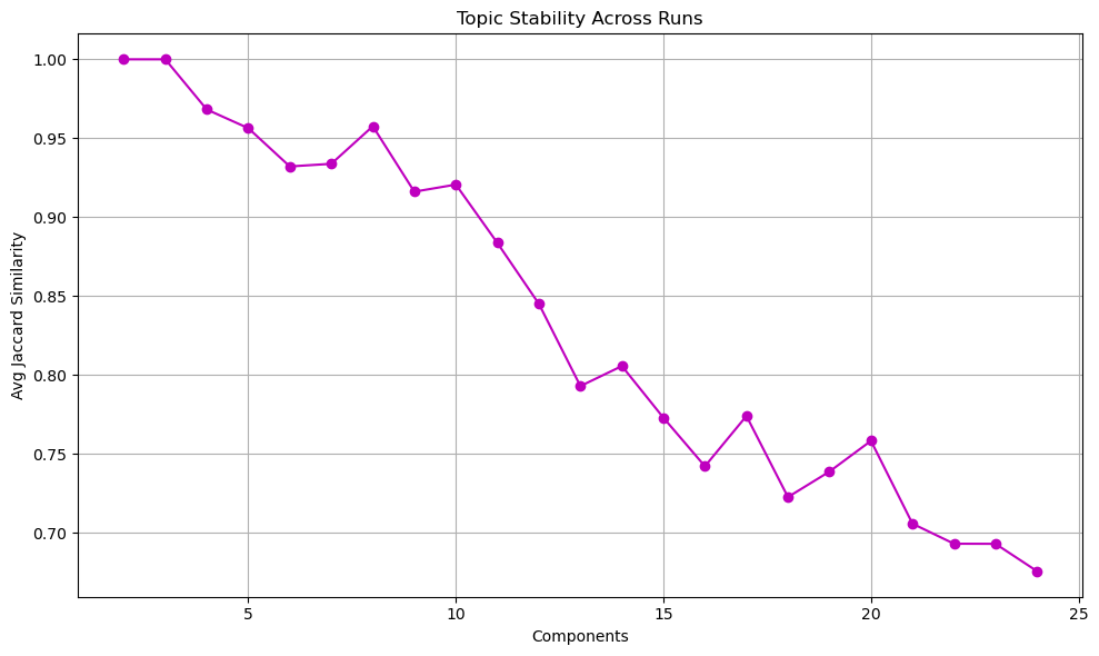
2. Evaluating Topic Quality...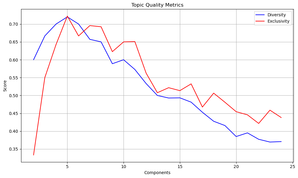
=== Analysis Complete ===
Based on the plots, manually set the optimal number of components.

Selected number of components: 5
The curves show a good trade-off between stability and diversity/exclusivity at a number of topics of 5. So we’ll set the number of topics to 5.
lda = LatentDirichletAllocation(
    n_components=5,  # Number of topics
    random_state=42,
    learning_method='online',
    max_iter=25
)

lda_output = lda.fit_transform(X_counts)

# Display topics
feature_names = count_vectorizer.get_feature_names_out()
for topic_idx, topic in enumerate(lda.components_):
    print(f"Topic #{topic_idx+1}:")
    print("|".join([feature_names[i] for i in topic.argsort()[:-11:-1]]))
    print()
Topic #1:
have|say|job|bill|the_united_states|even|now|get|money|year
Topic #2:
say|people|obama|support|want|make|vote|family|right|trump
Topic #3:
say|country|have|take|cost|get|america|come|american|congress
Topic #4:
government|work|say|spend|woman|republican|the|wisconsin|state|florida
Topic #5:
more|year|state|percent|have|say|time|pay|just|texasLet’s out the top statements per topic.
doc_topic_dist = lda.transform(X_counts)  # shape: (n_docs, n_topics)
liar['dominant_topic'] = doc_topic_dist.argmax(axis=1)
for topic_num in range(lda.n_components):
print(f"\n=== TOPIC {topic_num} ===")
top_indices = doc_topic_dist[:, topic_num].argsort()[::-1][:5]
for i in top_indices:
print(f"- {liar.iloc[i]['statement']}")
=== TOPIC 0 ===
- Russia and China "absolutely said pretty clearly" they would not keep economic sanctions on Iran if the United States "walked away from the deal.
- Joe Biden's sanctions on Russia "are riddled with loopholes and don't even start for 30 days. They have carve outs for the energy and financial sectors.
- Soybeans dropped 70 cents and corn 50 cents per bushel in two days, causing farmers to lose big money, "thanks to Biden's executive orders.
- The United States is "about to have the smallest Army since before WWII, the smallest Navy since WWI and the smallest Air Force ever.
- We've got 40 years of study now that show that, with a good preschool start, you're less likely to be on public dole, you're less likely to be in prison.

=== TOPIC 1 ===
- Says "Morgan Carroll opposed requiring convicted sex offenders to register their online profiles, making it harder to track online sex offenders and child predators.
- Says Bernie Sanders once said, "Instead of removing the conditions that make people depressed, modern society gives them antidepressant drugs.
- Says after leaving the White House, Hillary Clinton "was forced to return an estimated $200,000 in White House china, furniture and artwork that she had stolen.
- Photo shows Dianne Feinstein "bullying" Lisa Murkowski over "the now empty seat of the late Justice Ruth Bader Ginsburg.
- In the primary election, a "right-wing group spent more than $100,000,000 to support" Supreme Court Justice Rebecca Bradley.

=== TOPIC 2 ===
- Says Virginia Gov. Ralph Northam said, 'You will give up your guns, if you don't I'll have the National Guard cut your power, your phone lines, and your internet. Then, if you still refuse to comply I'll have you killed.'
- Ketanji Brown Jackson "says she gave pedophiles lighter sentences (because) it's different when they use computers vs mail to get volumes of child porn. This makes 'total sense' according to Jackson.
- The Trans-Pacific Partnership "knocks out 18,000 tariffs that other countries place on American products and goods.
- Says that Sen. Sherrod Brown is "out there egging on a lot of these protesters who are spitting on policemen and going to the bathroom on policemen's cars at these protests on Wall Street and other places.
- Protest vandalism in Richmond "all started two weeks ago when Mayor Stoney's police gassed - tear gassed - a peaceful crowd of protesters, moms and children, at 7:30 p.m. sharp.

=== TOPIC 3 ===
- Human error, such as skipping a community in the Wisconsin Supreme Court race, "is common in (the vote-tabulation) process.
- Says Pope Francis "was arrested Saturday in connection with an 80-count indictment of charges including possession of child pornography, human trafficking, incest, possession of drug paraphernalia and felony fraud.
- Between 2008 and 2014, "criminal aliens accounted for 38 percent of all murder convictions in the five states of California, Texas, Arizona, Florida and New York.
- If Russia, or some other entity, was hacking, why did the White House wait so long to act? Why did they only complain after Hillary lost?
- Says a California surfer was "alone, in the ocean," when he was arrested for violating the state's stay-at-home order.

=== TOPIC 4 ===
- A small business receiving a federal tax credit "to provide health care for its employees ... would be barred under the Stupak Amendment from allowing their employees to use ... the health care that they offer them for abortion.
- The top 1 percent of income earners pay 40 percent of all state income taxes, and those at the bottom pay little or nothing.
- Mark Kelly "voted to allow prison inmates to receive stimulus checks five separate times.
- Foxconn will not face oversight from any federal, state, or local agency to guarantee it complies with our wetlands protection laws.
- The House voted to cap insulin prices to $35/month, just $420 each year! Richard Hudson voted NO.
Looking at these LDA results, here’s what we can say:
Topic Analysis:
Topic 0: This topic appears focused on international relations, economic impacts, and national security. Key terms include “Russia,” “China,” “sanctions,” “Iran,” “United States,” and references to military size. This could represent discussions about foreign policy and defense.
Topic 1: This topic centers on political allegations, accusations against politicians, and controversial claims. Notable mentions include references to sex offenders, stolen items from the White House, and campaign spending. This seems to capture political attack messaging.
Topic 2: This topic contains content about protests, controversial political statements attributed to officials, and trade policy. It includes references to the Trans-Pacific Partnership, protesters, and alleged statements from political figures.
Topic 3: This topic appears to focus on claims about crime, election integrity, and controversial allegations. It includes references to “criminal aliens,” hacking claims, and alleged arrests. This seems to capture sensational or contested claims.
Topic 4: This topic appears to cover healthcare policy, taxation, and economic issues. It mentions healthcare, tax credits, stimulus checks, and specific policy proposals like insulin price caps.
Observations:
The topics show some coherence but also overlap considerably. For example, political figures (Obama, Trump) appear across multiple topics.
The model appears to have grouped statements more by subject matter than by other potential organizing principles like veracity or political leaning.
The top documents for each topic show how the LDA model is clustering similar content, though there’s still significant thematic overlap.
The road ahead:
we could consider adjusting the number of topics - The current 5 topics might be too few to capture distinct themes. We could running with 7-10 topics to see if we get clearer separation.
we could BERTopic next - Since our data has nuanced political content, BERTopic might capture more subtle semantic differences that word-frequency based LDA might miss.
🗺️ LDA results visualisation
Before moving to BERTopic, let’s first visualise the results of LDA.
# Prepare visualization
panel = pyLDAvis.prepare(
    topic_term_dists=lda.components_ / lda.components_.sum(axis=1)[:, None],  # normalize
    doc_topic_dists=lda.transform(X_counts),
    doc_lengths=(X_counts > 0).sum(axis=1).A1,  # number of tokens in each doc
    vocab=count_vectorizer.get_feature_names_out(),
    term_frequency=X_counts.sum(axis=0).A1
)

# To display inline in Jupyter Notebook:
pyLDAvis.display(panel)
Topic modeling : Moving beyond LDA to BERTopic
Our first attempt at uncovering thematic structure in political statements used LDA (Latent Dirichlet Allocation) — a classic, word-frequency-based topic modeling approach.
While it provided some insight, it fell short in a few key areas:
🧪 What we observed:
- Topics showed some coherence, but also a lot of semantic overlap — for example, figures like Obama or Trump appeared across multiple topics.
- It grouped statements by surface-level subject matter, but missed deeper patterns (like framing, stance, or veracity).
- Crucially, it required us to choose the number of topics manually, relying on heuristics or trial-and-error.
We even noted that increasing the number of topics (e.g. from 5 to 10) might improve clarity — but that still wouldn’t solve the core issue: LDA doesn’t “understand” meaning.
🚀 Enter BERTopic: Meaning-Aware Topic Modeling
To get richer, more distinct topics, we turned to BERTopic — a modern topic modeling technique that understands context and meaning using neural embeddings and clustering.
Rather than just counting co-occurring words, BERTopic groups statements that are semantically similar, even when they use different language.
🧠 What BERTopic Actually Does
BERTopic combines several powerful components:
1. Transformer-based Embeddings (for meaning)
It starts by turning each statement into a vector embedding — a list of numbers that represents its semantic meaning. This is done using a Transformer-based language model like BERT or MiniLM.
🧠 A Transformer is a type of deep neural network that processes text by attending to the relationships between all words in a sentence, allowing it to understand context far better than older models.
So phrases like: - “Healthcare premiums are rising”
- “Obamacare caused insurance costs to go up”
…are embedded close together, even if they don’t share words.
2. HDBSCAN Clustering (for automatic topic discovery)
Next, it uses HDBSCAN — a clustering algorithm related to DBSCAN — to group similar statements into topics:
- Finds dense clusters of similar texts in embedding space
- Automatically determines the number of topics
- Labels ambiguous or isolated statements as outliers (e.g., topic
-1)
This avoids the need for LDA-style guesswork about how many topics there should be.
3. c-TF-IDF Scoring (for distinctiveness)
Finally, BERTopic computes class-based TF-IDF (c-TF-IDF) to identify the most distinctive words for each topic:
- It merges all texts in a topic into one virtual document
- Then scores words that are frequent within the topic but rare across others
This yields interpretable keywords that make each topic easier to understand and label.
🔍 LDA vs. BERTopic: A Side-by-Side Comparison
Let’s illustrate how these methods differ using a small example.
Input Statements:
1. Obamacare led to rising healthcare premiums.
2. Health insurance rates have gone up in recent years.
3. Barack Obama announced the policy during his presidency.
LDA
- Based on word co-occurrence.
- Might place (1) and (3) in the same topic due to the word “Obama”.
- May not link (1) and (2), since they don’t share many exact words. Result: Topics influenced by shared surface terms, even if meanings diverge.
BERTopic
- Uses embeddings to understand that (1) and (2) both talk about healthcare costs.
- Understands that (3) is more biographical or political.
- Clusters (1) and (2) together, while (3) might land in a different cluster or become an outlier. Result: Topics grouped by meaning, not just vocabulary.
| Model | Grouping Logic | Grouping Result |
|---|---|---|
| LDA | Groups by word co-occurrence | Might group (1) and (3) together (both say “Obama”) |
| BERTopic | Groups by semantic similarity via embeddings | Groups (1) and (2) together (both about healthcare costs) |
🔄 Summary Comparison
| Feature | LDA | BERTopic |
|---|---|---|
| Text representation | Bag-of-Words | Sentence embeddings (semantic) |
| Context understanding | ❌ None | ✅ Yes |
| Synonym/generalization | ❌ No | ✅ Yes |
| Topic count | Must be set manually | Discovered automatically with HDBSCAN |
| Topic distinctiveness | Frequency-based | c-TF-IDF (topic-specific relevance) |
| Outlier handling | ❌ No | ✅ Yes (noise is excluded) |
| Visualization | Requires custom setup | ✅ Built-in and interactive |
💡 Why BERTopic Makes Sense for This Dataset
Political statements are: - Short - Often nuanced or rhetorically loaded - Use indirect phrasing or synonyms
This makes surface-level word clustering (like in LDA) brittle. BERTopic’s semantic approach is far better suited — helping us uncover meaningful, well-separated themes grounded in how people actually use language.
# Step 1: Extract raw statements
texts = liar_clean["statement"].tolist()

# Optional: Specify embedding model (MiniLM is a good default)
embedding_model = SentenceTransformer("all-MiniLM-L6-v2",cache_folder=os.getcwd())

# Step 2: Create BERTopic model with embedding model
topic_model = BERTopic(embedding_model=embedding_model, verbose=True)

# Step 3: Fit model on raw statements
topics, probs = topic_model.fit_transform(texts)

# Step 4: Explore topics
all_topics=topic_model.get_topic_info()
n_topics = all_topics.shape[0] - 1  # Subtract 1 to exclude the "-1" outlier topic
print(f"Number of topics found (excluding outliers): {n_topics}")
# OR:
print(f"Words for topic 0", topic_model.get_topic(0))  # Get words for topic 0

# Step 5: Visualize topics (interactively)
print("Visualising the top 10 topics")
topic_model.visualize_topics()topic_model.visualize_barchart(top_n_topics=10)topic_model.visualize_heatmap()topic_info = topic_model.get_topic_info()
topic_info| Topic | Count | Name | Representation | Representative_Docs | |
|---|---|---|---|---|---|
| 0 | -1 | 1894 | -1_the_to_says_in | [the, to, says, in, of, and, for, is, on, that] | [There was no effort” to get American experts … |
| 1 | 0 | 485 | 0_health_care_obamacare_medicare | [health, care, obamacare, medicare, insurance,… | [Wisconsin has “the number one health care sys… |
| 2 | 1 | 348 | 1_covid_19_vaccine_coronavirus | [covid, 19, vaccine, coronavirus, vaccines, va… | [Video shows that certain drinks can “test pos… |
| 3 | 2 | 305 | 2_election_vote_voter_ballots | [election, vote, voter, ballots, votes, voting… | [In Iowa, “since we have put a number of the v… |
| 4 | 3 | 208 | 3_school_schools_education_public | [school, schools, education, public, graduatio… | [Mayor Fung wants to punish our children’s edu… |
| … | … | … | … | … | … |
| 68 | 67 | 11 | 67_formula_baby_shortage_obesity | [formula, baby, shortage, obesity, current, ki… | [Due to the baby formula shortage Tricare will… |
| 69 | 68 | 11 | 68_fund_rainy_budget_budgets | [fund, rainy, budget, budgets, governor, day, … | [As state Commerce secretary, Mary Burke draft… |
| 70 | 69 | 11 | 69_gender_old_consent_boy | [gender, old, consent, boy, school, trans, gir… | [Assertions that it makes no difference whethe… |
| 71 | 70 | 11 | 70_virginia_west_virginians_moving | [virginia, west, virginians, moving, average, … | [West Virginia added the highest percentage of… |
| 72 | 71 | 10 | 71_jefferson_thomas_written_government | [jefferson, thomas, written, government, restr… | [Thomas Jefferson said, “That government is be… |
73 rows × 5 columns
BERTopic finds 74 topics (aside from outliers)! The distribution shows a long tail pattern typical of news/political discourse where a few major issues dominate but many niche topics exist: the predominant topics seem to be healthcare/Obamacare/Medicare (topic 0), Covid 19/vaccines (topic 1), elections/voting - clearly tied to voting or election fraud narratives (topic 2), education/schools (topic 3) and some niche topics are NFL Anthem protests or Carolina North HB21 BERTopic also finds many outliers (there are more outliers than there are statements in the top topic!), either illustrating the diversity od topics and inherent noisiness of the data or suggesting that we might need to consider different embeddings or optimize the minimum topic size parameter for BERTopic to better capture the data structure.
Just as with LDA, we want to see which words are more representative of each topic and which are the top statements associated with each topic.
def get_representative_docs(topic_model, texts, topics, probs, n=5):
    """
    Get the most representative documents for each topic.

    Parameters:
    -----------
    topic_model : BERTopic model
        The fitted BERTopic model
    texts : list
        List of original text documents
    topics : list
        List of topic assignments for each document
    probs : list
        List of probability distributions for each document
    n : int, optional
        Number of representative documents to return per topic

    Returns:
    --------
    dict
        Dictionary mapping topic IDs to lists of representative documents
    """
    topic_to_docs = {}

    # Exclude outlier topic (-1) and get unique topics
    unique_topics = set(topics)
    if -1 in unique_topics:
        unique_topics.remove(-1)

    for topic_id in unique_topics:
        # Get document indices for this topic
        indices = [i for i, t in enumerate(topics) if t == topic_id]

        # Skip if no documents in this topic
        if not indices:
            continue

        # Get probabilities for these documents
        # Each document's probability of belonging to this topic
        topic_probs = []
        for i in indices:
            # Find the probability for this topic
            # The structure depends on how BERTopic returns probabilities
            if isinstance(probs[i], list) and len(probs[i]) > 0:
                if isinstance(probs[i][0], tuple):
                    # If probs is a list of tuples like [(topic_id, prob), ...]
                    for t, p in probs[i]:
                        if t == topic_id:
                            topic_probs.append(p)
                            break
                    else:
                        topic_probs.append(0.0)  # Topic not found in probabilities
                else:
                    # If probs is a list of probabilities in order of topics
                    try:
                        topic_idx = list(topic_model.topic_mapper_.index_to_topic_.values()).index(topic_id)
                        topic_probs.append(probs[i][topic_idx])
                    except:
                        topic_probs.append(0.0)  # Topic not found in mapping
            else:
                topic_probs.append(0.0)  # No probability data

        # If we couldn't get reliable probabilities, use all documents
        if all(p == 0.0 for p in topic_probs):
            sorted_indices = indices[:n]
        else:
            # Sort by probability (highest first) and get top n
            sorted_indices = [indices[i] for i in np.argsort(topic_probs)[::-1][:n]]

        # Store documents
        topic_to_docs[topic_id] = [texts[i] for i in sorted_indices]

    return topic_to_docs

def display_topics_with_docs(topic_model, texts, topics, probs, n_docs=3, n_words=10):
    """
    Display topics with their representative documents.

    Parameters:
    -----------
    topic_model : BERTopic model
        The fitted BERTopic model
    texts : list
        List of original text documents
    topics : list
        List of topic assignments for each document
    probs : list
        List of probability distributions for each document
    n_docs : int, optional
        Number of representative documents to show per topic
    n_words : int, optional
        Number of words to show for each topic
    """
    # Get topic information
    topic_info = topic_model.get_topic_info()

    # Get representative documents
    rep_docs = get_representative_docs(topic_model, texts, topics, probs, n=n_docs)

    # Create a clean display
    print(f"{'='*80}")
    print(f"{'TOPIC SUMMARY':^80}")
    print(f"{'='*80}")

    # Display info for each topic, sorted by size (excluding -1)
    for _, row in topic_info[topic_info['Topic'] != -1].iterrows():
        topic_id = row['Topic']
        topic_name = row['Name']
        topic_size = row['Count']

        # Get words for this topic
        topic_words = topic_model.get_topic(topic_id)
        words_str = ", ".join([f"{word} ({score:.3f})" for word, score in topic_words[:n_words]])

        print(f"\nTOPIC {topic_id}: {topic_name} ({topic_size} documents)")
        print(f"Keywords: {words_str}")

        # Display representative documents
        if topic_id in rep_docs:
            print("\nRepresentative documents:")
            for i, doc in enumerate(rep_docs[topic_id]):
                # Limit document length for display
                display_doc = doc[:200] + "..." if len(doc) > 200 else doc
                print(f"{i+1}. {display_doc}")
        else:
            print("\nNo representative documents found for this topic.")

        print(f"{'-'*80}")

    # Display info for outlier topic if it exists
    if -1 in topics:
        outlier_count = topics.count(-1)
        print(f"\nOUTLIER TOPIC: -1 ({outlier_count} documents)")
        print("Documents that don't fit well into any topic")
        print(f"{'-'*80}")

# Example usage:
# display_topics_with_docs(topic_model, texts, topics, probs)

# To save the results to a file:
def save_topics_with_docs(topic_model, texts, topics, probs, n_docs=5, n_words=10, filename="topic_results.md"):
    """Save topics with their representative documents to a markdown file."""
    with open(filename, "w") as f:
        f.write("# BERTopic Results\n\n")

        # Get topic information
        topic_info = topic_model.get_topic_info()

        # Get representative documents
        rep_docs = get_representative_docs(topic_model, texts, topics, probs, n=n_docs)

        # Display info for each topic, sorted by size (excluding -1)
        for _, row in topic_info[topic_info['Topic'] != -1].iterrows():
            topic_id = row['Topic']
            topic_name = row['Name']
            topic_size = row['Count']

            # Get words for this topic
            topic_words = topic_model.get_topic(topic_id)
            words_str = ", ".join([f"{word} ({score:.3f})" for word, score in topic_words[:n_words]])

            f.write(f"\n## TOPIC {topic_id}: {topic_name} ({topic_size} documents)\n\n")
            f.write(f"**Keywords:** {words_str}\n\n")

            # Display representative documents
            if topic_id in rep_docs:
                f.write("### Representative documents:\n\n")
                for i, doc in enumerate(rep_docs[topic_id]):
                    f.write(f"{i+1}. {doc}\n\n")
            else:
                f.write("No representative documents found for this topic.\n\n")

            f.write("---\n")
display_topics_with_docs(topic_model, texts, topics, probs, n_docs=3, n_words=8)
# Save results to a markdown file for easier sharing/analysis
save_topics_with_docs(topic_model, texts, topics, probs, n_docs=5, n_words=10,
filename="liar_topics_analysis.md")================================================================================
TOPIC SUMMARY
================================================================================
TOPIC 0: 0_health_care_obamacare_medicare (485 documents)
Keywords: health (0.038), care (0.036), obamacare (0.027), medicare (0.026), insurance (0.021), social (0.015), medicaid (0.014), security (0.014)
Representative documents:
1. A small business receiving a federal tax credit "to provide health care for its employees ... would be barred under the Stupak Amendment from allowing their employees to use ... the health care that t...
2. Says Mark Udall "decided Obamacare. ... He passed Obamacare with his vote.
3. Says Bernie Sanders once said, "Instead of removing the conditions that make people depressed, modern society gives them antidepressant drugs.
--------------------------------------------------------------------------------
TOPIC 1: 1_covid_19_vaccine_coronavirus (348 documents)
Keywords: covid (0.060), 19 (0.048), vaccine (0.033), coronavirus (0.026), vaccines (0.019), vaccinated (0.016), people (0.014), are (0.014)
Representative documents:
1. Video shows that certain drinks can "test positive" for COVID-19 when using at-home COVID-19 tests.
2. The AstraZeneca COVID-19 vaccine contains a Bluetooth microchip.
3. Says drinking a "6-ounce glass of tonic water each night before bed" will help alleviate restless legs syndrome.
--------------------------------------------------------------------------------
TOPIC 2: 2_election_vote_voter_ballots (305 documents)
Keywords: election (0.029), vote (0.026), voter (0.022), ballots (0.021), votes (0.019), voting (0.018), voters (0.017), in (0.016)
Representative documents:
1. Canadian-born Ted Cruz "has had a double passport.
2. In certain swing states, there were more votes than people who voted, and in big numbers.
3. Electronic voting machines didn't allow people to vote" in Maricopa County, Arizona.
--------------------------------------------------------------------------------
TOPIC 3: 3_school_schools_education_public (208 documents)
Keywords: school (0.043), schools (0.035), education (0.031), public (0.021), graduation (0.020), college (0.020), students (0.019), funding (0.018)
Representative documents:
1. Richmond teachers have not gotten a raise "for almost 10 years.
2. Inner-city students "fall back and don't succeed, whereas if there was a less intensive track, they would.
3. Says "Gary Johnson and the Libertarian Party want to get rid of the public school system.
--------------------------------------------------------------------------------
TOPIC 4: 4_obama_barack_iran_president (173 documents)
Keywords: obama (0.046), barack (0.033), iran (0.023), president (0.023), nuclear (0.019), muslim (0.016), to (0.015), said (0.014)
Representative documents:
1. Barack Obama: I'm 'the First Sitting American President to Come From Kenya.'
2. Russia and China "absolutely said pretty clearly" they would not keep economic sanctions on Iran if the United States "walked away from the deal.
3. Says Barack Obama is "trying to slash funding for the Armed Pilots Program designed to prevent terror attacks.
--------------------------------------------------------------------------------
TOPIC 5: 5_debt_trillion_deficit_spending (126 documents)
Keywords: debt (0.078), trillion (0.042), deficit (0.032), spending (0.028), national (0.027), budget (0.022), federal (0.019), the (0.018)
Representative documents:
1. Sheldon Whitehouse's failure of leadership, the adding of almost $8 trillion in debt in his first full term, is shameful...
2. We have a national debt the size of our nation's economy for the first time since World War II.
3. The largest contributor to the debt ceiling, or to our deficit, has been the Trump tax cuts.
--------------------------------------------------------------------------------
TOPIC 6: 6_abortion_parenthood_planned_abortions (110 documents)
Keywords: abortion (0.074), parenthood (0.044), planned (0.041), abortions (0.038), women (0.024), birth (0.023), baby (0.022), pro (0.021)
Representative documents:
1. Planned Parenthood "is an organization that funnels millions of dollars in political contributions to pro-abortion candidates.
2. The House health care bill provides for "free abortion services, and probably forced participation in abortions by members of the medical profession.
3. Says he didn't call Dr. George Tiller a baby killer, as liberal groups charge, but was merely reporting what "some prolifers branded him.
--------------------------------------------------------------------------------
TOPIC 7: 7_crime_gun_violent_killed (109 documents)
Keywords: crime (0.046), gun (0.029), violent (0.026), killed (0.026), rate (0.023), in (0.022), violence (0.018), murder (0.018)
Representative documents:
1. Most of your serial killers, most of your people who commit domestic violence, they start off by abusing animals.
2. There are places in America that are among the most dangerous in the world. You go to places like Oakland. Or Ferguson. The crime numbers are worse. Seriously.
3. Says the manager of a Checkers in Miami Gardens, Fla., killed 10 employees.
--------------------------------------------------------------------------------
TOPIC 8: 8_jobs_created_job_000 (108 documents)
Keywords: jobs (0.082), created (0.045), job (0.031), 000 (0.029), ohio (0.028), sector (0.024), since (0.021), more (0.018)
Representative documents:
1. We've had the same leadership in the Travis County DA's office for 30 years.
2. There was a "loss of eight million jobs during the Bush eight years.
3. There are giant human caucasian skeletons in Ohio that predate any known civilizations.
--------------------------------------------------------------------------------
TOPIC 9: 9_biden_joe_video_shows (100 documents)
Keywords: biden (0.140), joe (0.113), video (0.046), shows (0.035), hunter (0.026), president (0.023), his (0.023), he (0.017)
Representative documents:
1. Joe Biden's wide open southern border" is to blame for fentanyl deaths in the U.S.
2. Says Jill Biden said, "Whatever is on Hunter's laptop is not important.
3. There is no Biden presidency. The real Biden was executed for his crimes long ago along with Clinton.
--------------------------------------------------------------------------------
TOPIC 10: 10_gun_background_checks_guns (79 documents)
Keywords: gun (0.068), background (0.053), checks (0.037), guns (0.033), nra (0.026), you (0.026), ban (0.024), firearms (0.024)
Representative documents:
1. California's Proposition 63 would "CRIMINALIZE the sharing of ammunition between friends who may be hunting or shooting together.
2. The New START treaty was passed despite significant concerns among some people in the State and Defense Departments.
3. A law that mandates fingerprinting for gun purchasers is "a requirement that's reduced gun crimes in the five states where it's the law.
--------------------------------------------------------------------------------
TOPIC 11: 11_border_immigration_mexico_illegal (70 documents)
Keywords: border (0.092), immigration (0.029), mexico (0.027), illegal (0.024), patrol (0.022), secure (0.020), we (0.019), illegally (0.018)
Representative documents:
1. Says President Donald Trump said asylum seekers "aren't people. These are animals.
2. The Obama administration "manipulated deportation data to make it appear that the Border Patrol was deporting more illegal immigrants than the Bush administration.
3. A lot of these migrants that are coming, we have no way to screen their backgrounds for either health or for security.
--------------------------------------------------------------------------------
TOPIC 12: 12_climate_change_warming_ice (60 documents)
Keywords: climate (0.067), change (0.049), warming (0.046), ice (0.041), global (0.034), earth (0.032), hoax (0.023), emissions (0.022)
Representative documents:
1. Asteroid warning: NASA tracks a 4KM killer rock on approach - Could end human civilisation.
2. Carbon dioxide is not "a primary contributor to the global warming that we see.
3. We need to also recognize that we just had two of the coldest years, biggest drop in global temperatures that we have had since the 1980s, the biggest in the last 100 years. We don't talk about that.
--------------------------------------------------------------------------------
TOPIC 13: 13_ukraine_russian_video_moon (58 documents)
Keywords: ukraine (0.096), russian (0.054), video (0.052), moon (0.047), putin (0.045), shows (0.038), landing (0.036), ufo (0.031)
Representative documents:
1. Photo shows a Russian tank Ukrainians are selling on eBay.
2. NASA Curiosity finds Nazi helmet on Mars.
3. A video shows a real angel in the sky in Palestine.
--------------------------------------------------------------------------------
TOPIC 14: 14_taxes_tax_kaine_tim (57 documents)
Keywords: taxes (0.086), tax (0.067), kaine (0.052), tim (0.049), increase (0.043), raise (0.042), raised (0.029), voted (0.023)
Representative documents:
1. Says Wendy's founder "Dave Thomas left the state literally on his deathbed to avoid the estate tax.
2. Says Jeanne Shaheen "voted to pave the way for a new national energy tax.
3. Says U.S. Senate rival Tammy Baldwin supports a "tax increase that President Obama says" would cost middle-class families $3,000 per year.
--------------------------------------------------------------------------------
TOPIC 15: 15_tax_taxes_cuts_property (53 documents)
Keywords: tax (0.085), taxes (0.030), cuts (0.025), property (0.023), relief (0.023), cut (0.019), republican (0.019), irs (0.018)
Representative documents:
1. If you or your family spends $28 a day — prepare to be under constant audit by the IRS.
2. We've got a personal tax system that's so complicated it costs Americans about $500 billion a year to comply with the current tax code.
3. GDP is booming. Let's spread the prosperity to the middle class with big #TaxCuts. Our #TaxReform package doubles standard deduction, brings $$$ back home, and reduces rates for ALL taxpayers. We will...
--------------------------------------------------------------------------------
TOPIC 16: 16_photo_shows_epstein_jeffrey (51 documents)
Keywords: photo (0.107), shows (0.074), epstein (0.044), jeffrey (0.038), photos (0.035), posing (0.034), michelle (0.028), shirt (0.028)
Representative documents:
1. Photo shows Queen Elizabeth II being carried across a river by African porters.
2. Photo shows former President Donald Trump "dancing with a 13-year-old girl" on Jeffrey Epstein's private island.
3. Says Nancy Pelosi and Beto O'Rourke were photographed with El Chapo.
--------------------------------------------------------------------------------
TOPIC 17: 17_pelosi_nancy_kamala_harris (48 documents)
Keywords: pelosi (0.102), nancy (0.086), kamala (0.048), harris (0.047), schiff (0.039), resign (0.037), adam (0.032), video (0.032)
Representative documents:
1. Kamala Harris resigns in shock after Biden's 'mandatory' border trip…Trump jails 'corrupt' VP.
2. Democrats Filing TREASON Charges Against Trump, McConnell, Giuliani, & Comey.
3. Pelosi sinks to new low, tells Dems: if you have to lie to voters to win, do it.
--------------------------------------------------------------------------------
TOPIC 18: 18_clinton_hillary_she_emails (47 documents)
Keywords: clinton (0.104), hillary (0.097), she (0.042), emails (0.038), fbi (0.033), her (0.032), email (0.029), laughing (0.024)
Representative documents:
1. Says "Hillary Clinton filed for divorce In New York courts.
2. The FBI has reopened its investigation into Hillary Clinton ... and discovered another 650,000 emails.
3. Says Hillary Clinton is "wrong" to say he mocked a disabled reporter.
--------------------------------------------------------------------------------
TOPIC 19: 19_coal_solar_energy_electric (47 documents)
Keywords: coal (0.081), solar (0.064), energy (0.053), electric (0.042), power (0.039), wind (0.032), gas (0.024), electricity (0.024)
Representative documents:
1. Puerto Rico's electric grid and their electric generating plant was dead before the storms ever hit. It was in very bad shape. It was in bankruptcy. It had no money. It was largely -- you know, it was...
2. China will be allowed to build hundreds of additional coal plants. So we can't build the plants, but they can, according to this (Paris) agreement.
3. Energy nominee Steven Chu has called coal "his worst nightmare.
--------------------------------------------------------------------------------
TOPIC 20: 20_wisconsin_income_growth_walker (45 documents)
Keywords: wisconsin (0.139), income (0.032), growth (0.031), walker (0.026), scott (0.022), player (0.021), midwest (0.019), jobs (0.019)
Representative documents:
1. Wisconsin is not as obese as the national average is. The national average, 35.7 percent of the population is obese. In Wisconsin, it's closer to 26 percent.
2. The sale of more than 600,000 Wisconsin deer licenses shows that Wisconsin's hunters are the "eighth largest army in the world.
3. Wisconsin is "dead last in income growth" among midwestern states during Gov. Scott Walker's term.
--------------------------------------------------------------------------------
TOPIC 21: 21_wage_minimum_hour_women (44 documents)
Keywords: wage (0.084), minimum (0.068), hour (0.049), women (0.048), wages (0.047), cents (0.041), average (0.038), men (0.037)
Representative documents:
1. Under Barack Obama and the big government economy, the median wage for women has dropped $733.
2. Raising the national minimum wage to $15 per hour "would destroy up to 3.7 million jobs.
3. A Congressional Budget Office report says President Barack Obama's executive order to raise the minimum wage for new federal contract workers "will cost the economy 500,000 jobs.
--------------------------------------------------------------------------------
TOPIC 22: 22_money_campaign_million_pac (44 documents)
Keywords: money (0.035), campaign (0.032), million (0.030), pac (0.030), foundation (0.025), clinton (0.024), trump (0.023), donors (0.021)
Representative documents:
1. During "the recent global warming summit in Copenhagen, Nancy Pelosi and others stayed at a five-star hotel on a trip costing nearly $10,000 per person.
2. Says Sen. Elizabeth Warren "lives in a $5.4 million mansion.
3. Says his campaign hasn't accepted corporate PAC money and isn't funded by "special interests.
--------------------------------------------------------------------------------
TOPIC 23: 23_mccain_john_he_against (42 documents)
Keywords: mccain (0.123), john (0.058), he (0.045), against (0.027), equal (0.026), said (0.023), negative (0.022), troops (0.022)
Representative documents:
1. Says Claire McCaskill "voted against including health records in the background check system.
2. We haven't yet taken out a negative ad.
3. Says McCain was a "Hanoi Hilton songbird" who collaborated with the enemy.
--------------------------------------------------------------------------------
TOPIC 24: 24_austin_texas_city_residents (38 documents)
Keywords: austin (0.087), texas (0.080), city (0.051), residents (0.028), mayor (0.027), antonio (0.027), says (0.024), council (0.023)
Representative documents:
1. Says Texas Rep. Terry Meza said changing the castle doctrine is meant to create a "peaceful" transfer of property from victims to thieves
2. Austin is "effectively" imposing "a ban on barbecue restaurants.
3. Russia has more diversity in its governmental representation than we do in Texas.
--------------------------------------------------------------------------------
TOPIC 25: 25_fbi_espionage_investigation_waterboarding (37 documents)
Keywords: fbi (0.054), espionage (0.035), investigation (0.027), waterboarding (0.027), warrant (0.025), james (0.023), news (0.023), spy (0.020)
Representative documents:
1. The White House fully cooperated with the Special Counsel's investigation.
2. The FBI said (former national security adviser Michael Flynn) wasn't lying.
3. Mark Kirk's claim of national security expertise is "based on his military record which he lied about at least 10 times.
--------------------------------------------------------------------------------
TOPIC 26: 26_poverty_homeownership_wealth_rate (36 documents)
Keywords: poverty (0.109), homeownership (0.036), wealth (0.036), rate (0.035), poor (0.034), black (0.034), african (0.033), white (0.029)
Representative documents:
1. 70% of Americans in poverty are white.
2. Says California has "30% or a third of the country's people living at or below the poverty level.
3. Black Friday originated in 1904 when enslaved people were sold at a discount to boost the economy.
--------------------------------------------------------------------------------
TOPIC 27: 27_unemployment_rate_black_lowest (35 documents)
Keywords: unemployment (0.204), rate (0.070), black (0.037), lowest (0.036), unemployed (0.036), sees (0.030), percent (0.028), been (0.028)
Representative documents:
1. Says the Congressional Budget Office said "unemployment could top 9 percent in 2013
2. Hispanic unemployment has been ticking down from an all-time high of 13.9 percent because of the policies we've implemented.
3. Chicago maintained the lowest unemployment rate through most of 2021 of any large American city.
--------------------------------------------------------------------------------
TOPIC 28: 28_stimulus_checks_projects_ants (34 documents)
Keywords: stimulus (0.182), checks (0.050), projects (0.030), ants (0.029), package (0.029), went (0.029), spent (0.027), alaska (0.025)
Representative documents:
1. Says Steve Jobs was responsible for creating more jobs than the stimulus bill.
2. Catherine Cortez Masto "was the deciding vote" to send COVID-19 stimulus checks to more than 1 million prisoners.
3. $2,000 stimulus checks were due on Jan. 19.
--------------------------------------------------------------------------------
TOPIC 29: 29_antifa_matter_lives_school (32 documents)
Keywords: antifa (0.144), matter (0.042), lives (0.041), school (0.040), parents (0.036), shooter (0.036), terrorist (0.035), black (0.032)
Representative documents:
1. Black Lives Matter and antifa set Catholic church on fire in Minneapolis.
2. The Nashville, Tennessee, school shooter was Samantha Hyde.
3. 12 white female bodies in garage freezer tagged 'Black Lives Matter.'
--------------------------------------------------------------------------------
TOPIC 30: 30_oil_gallon_gas_pump (32 documents)
Keywords: oil (0.125), gallon (0.048), gas (0.047), pump (0.036), cents (0.036), prices (0.034), energy (0.033), russia (0.032)
Representative documents:
1. Soybeans dropped 70 cents and corn 50 cents per bushel in two days, causing farmers to lose big money, "thanks to Biden's executive orders.
2. We have doubled our (oil) imports from Russia in the last year.
3. Ron Klein "sponsored an amendment that specifically allows price gouging.
--------------------------------------------------------------------------------
TOPIC 31: 31_food_milk_fast_fda (31 documents)
Keywords: food (0.079), milk (0.044), fast (0.041), fda (0.034), store (0.028), shortage (0.027), salmonella (0.023), eggs (0.023)
Representative documents:
1. Not one illness has been reported from raw milk in" Texas "in more than four years. A total of six illnesses have occurred in the last 20 years.
2. McDonald's uses potatoes sprayed with a highly toxic pesticide called Monitor.
3. The current (agriculture) commissioner allowed tainted beef to be sent to school cafeterias.
--------------------------------------------------------------------------------
TOPIC 32: 32_defense_aid_afghanistan_spend (30 documents)
Keywords: defense (0.067), aid (0.043), afghanistan (0.041), spend (0.039), military (0.038), gives (0.037), israel (0.035), spent (0.034)
Representative documents:
1. We spend three times more on entitlements and debt services than we do on defense.
2. We have one of the most expensive General Assemblies, per capita, in the entire country.
3. We have spent $7 trillion, trillion with a T, $7 trillion in the Middle East.
--------------------------------------------------------------------------------
TOPIC 33: 33_capitol_protesters_protesting_protest (30 documents)
Keywords: capitol (0.072), protesters (0.059), protesting (0.057), protest (0.051), riots (0.047), shows (0.046), riot (0.035), peaceful (0.035)
Representative documents:
1. The Simpsons predicted the Capitol riots
2. A photo shows two men on the run who pretend to be homeless and then "attack and rob you.
3. Protest vandalism in Richmond "all started two weeks ago when Mayor Stoney's police gassed - tear gassed - a peaceful crowd of protesters, moms and children, at 7:30 p.m. sharp.
--------------------------------------------------------------------------------
TOPIC 34: 34_jersey_new_jobs_states (29 documents)
Keywords: jersey (0.111), new (0.077), jobs (0.034), states (0.029), state (0.029), sector (0.023), growth (0.022), york (0.020)
Representative documents:
1. Because of its higher minimum wage, New York State is "already showing signs of various companies picking up and leaving.
2. Columbia, Mo., is "one of the fastest growing cities in the region, the only city in the state to grow jobs faster than the nation as a whole.
3. This decision is an unfortunate example of why those of us in Montpelier need to work together to make Vermont a more affordable place to do business and make sure our policies help businesses thrive ...
--------------------------------------------------------------------------------
TOPIC 35: 35_water_gallons_loophole_waters (29 documents)
Keywords: water (0.135), gallons (0.056), loophole (0.028), waters (0.028), drinking (0.027), saved (0.025), clean (0.025), flow (0.023)
Representative documents:
1. Onion Creek's highest flow rate" on a recent night of flooding "was 120,000 cubic feet per second, which is nearly double the average flow rate of Niagara Falls.
2. The Atlanta area's water planning district "is now the national leader in conservation.
3. The train that derailed in Ohio was carrying "over 300,000 gallons of a chemical that was banned in 1974.
--------------------------------------------------------------------------------
TOPIC 36: 36_income_pay_tax_taxes (28 documents)
Keywords: income (0.094), pay (0.077), tax (0.076), taxes (0.049), earners (0.047), percent (0.036), taxed (0.036), americans (0.031)
Representative documents:
1. The top 1 percent of income earners pay 40 percent of all state income taxes, and those at the bottom pay little or nothing.
2. We're the most highly taxed nation in the world.
3. As a U.S. senator with salary and perks, #Bernie is in the top 1 percent, but still paid only 13 percent in taxes last year.
--------------------------------------------------------------------------------
TOPIC 37: 37_marriage_equality_miss_marry (27 documents)
Keywords: marriage (0.100), equality (0.045), miss (0.040), marry (0.040), married (0.035), husband (0.033), donald (0.032), webster (0.028)
Representative documents:
1. Says you can determine a bell pepper's gender by its "bumps.
2. Kavanaugh accuser's husband breaks his silence, exposes 'sick issue' his wife has.
3. Husbands rarely beat up their wives. Single women get beaten up more.
--------------------------------------------------------------------------------
TOPIC 38: 38_romney_mitt_massachusetts_bain (27 documents)
Keywords: romney (0.187), mitt (0.167), massachusetts (0.061), bain (0.042), capital (0.031), bankruptcy (0.026), maxwell (0.025), plant (0.023)
Representative documents:
1. Says Romney and Bain Capital drove KB Toys into bankruptcy by loading it up with debt.
2. Epstein's recruiter Ghislaine Maxwell's father Robert Maxwell gave Mitt Romney his first $2M investment and started him in business.
3. Mitt Romney "supervised a company guilty of massive Medicare fraud.
--------------------------------------------------------------------------------
TOPIC 39: 39_marijuana_medical_legalizing_use (27 documents)
Keywords: marijuana (0.217), medical (0.059), legalizing (0.039), use (0.036), pot (0.035), teenager (0.029), smoking (0.029), recreational (0.029)
Representative documents:
1. Twenty-five percent of our kids in foster care are there because their parents are involved in drugs.
2. In one Colorado hospital, 50 percent of newborns tested had marijuana in their system.
3. Medical-grade marijuana alone will not get that patient 'high,' no matter what level of THC, CBD or any other compound is found in the plant.
--------------------------------------------------------------------------------
TOPIC 40: 40_road_lanes_milwaukee_built (26 documents)
Keywords: road (0.059), lanes (0.057), milwaukee (0.054), built (0.038), bridges (0.034), wi (0.033), rail (0.033), public (0.032)
Representative documents:
1. I took on the worst road system in the country, according to Trucker's magazine. When I left, they said it was the most improved road system in the country.
2. Fifteen years ago, you couldn't even get a pizza delivered in that neighborhood.
3. We don't have bridges being built" in the United States.
--------------------------------------------------------------------------------
TOPIC 41: 41_ocasio_alexandria_cortez_communism (26 documents)
Keywords: ocasio (0.053), alexandria (0.053), cortez (0.052), communism (0.040), marxist (0.040), socialists (0.040), democratic (0.039), socialist (0.038)
Representative documents:
1. Say New Jersey Reps. Donald Payne and Frank Pallone are "socialists who are openly serving in the U.S. Congress.
2. Says Alexandria Ocasio-Cortez tweeted, "Let's begin 'The Purge' to roundup all Conservative traitors.
3. Says Bernie Sanders "collaborated with Marxist regimes in the Soviet Union, Nicaragua and Cuba.
--------------------------------------------------------------------------------
TOPIC 42: 42_court_supreme_justices_election (24 documents)
Keywords: court (0.112), supreme (0.103), justices (0.056), election (0.047), confirmed (0.046), nominees (0.043), judges (0.040), bench (0.038)
Representative documents:
1. It has been 80 years since a Supreme Court vacancy was nominated and confirmed in an election year. There is a long tradition that you don't do this in an election year.
2. We've got four Supreme Court justices who … signed their name to a declaration that Americans have no fundamental right to self-defense.
3. Cheri Beasley "vacated" a man's death sentence and "threw out" the indictment in a child assault case.
--------------------------------------------------------------------------------
TOPIC 43: 43_perry_rick_texas_governor (23 documents)
Keywords: perry (0.219), rick (0.176), texas (0.040), governor (0.038), gov (0.036), binational (0.034), forum (0.030), lobbyists (0.029)
Representative documents:
1. Says Rick Perry and the Republican-controlled Texas Legislature "managed to slash the budget of the volunteer fire departments in our state by 75 percent in the last legislative session," reducing the...
2. Gov. Rick Perry "has overseen the highest Texas unemployment in 22 years.
3. Says Rick Perry is "spending more money than the state takes in, covering his deficits with record borrowing.
--------------------------------------------------------------------------------
TOPIC 44: 44_barack_obama_president_deported (23 documents)
Keywords: barack (0.077), obama (0.065), president (0.060), deported (0.059), immigration (0.056), authority (0.051), executive (0.041), deportation (0.037)
Representative documents:
1. President Barack Obama has the "power to stop deportation for all undocumented immigrants in this country.
2. President Obama said "22 times" he could not authorize immigration reform by executive order.
3. Latina who enthusiastically supported Donald Trump on stage in Las Vegas in October 2015 has been deported.
--------------------------------------------------------------------------------
TOPIC 45: 45_never_worked_obama_barack (22 documents)
Keywords: never (0.128), worked (0.059), obama (0.048), barack (0.040), encouraged (0.039), president (0.039), business (0.036), no (0.035)
Representative documents:
1. Says Barack Obama "is the first president in modern history not to have a single year of 3 percent growth.
2. There was no panhandling when I left office.
3. 92 percent" of President Barack Obama's administration has "never worked outside government.
--------------------------------------------------------------------------------
TOPIC 46: 46_drug_heroin_overdose_drugs (22 documents)
Keywords: drug (0.068), heroin (0.057), overdose (0.057), drugs (0.053), overdoses (0.047), throw (0.044), death (0.036), fentanyl (0.031)
Representative documents:
1. Says police are warning shoppers to use wipes to clean their carts over deadly risk of fentanyl residue.
2. So now they take drugs, literally, and they throw it, a hundred pounds of drugs. They throw it over the wall, they have catapults, but they throw it over the wall, and it lands and it hits somebody on...
3. 100% of heroin/fentanyl epidemic is because we don't have a WALL.
--------------------------------------------------------------------------------
TOPIC 47: 47_african_men_prison_whites (22 documents)
Keywords: african (0.113), men (0.064), prison (0.054), whites (0.052), arrested (0.047), blacks (0.047), likely (0.046), americans (0.046)
Representative documents:
1. ''Over 40 percent of African-American men in (Milwaukee County) have been going to prison for low-level drug offenses, and I think a hundred times that in the city of Madison.
2. In the 513 days between Trayvon dying, and today's verdict, 11,106 African-Americans have been murdered by other African-Americans.
3. There are more young black males involved in the criminal justice system than there are in higher education.
--------------------------------------------------------------------------------
TOPIC 48: 48_drilling_biden_offshore_pipeline (20 documents)
Keywords: drilling (0.112), biden (0.062), offshore (0.059), pipeline (0.052), oil (0.052), shale (0.045), crack (0.045), joe (0.044)
Representative documents:
1. A Costco gas pump screen said "Don't blame us. Blame Joe Biden.
2. NASA just announced a 100-foot-wide fissure-crack just opened up Yellowstone volcano in 24 hours.
3. I have always said that I would be for drilling.
--------------------------------------------------------------------------------
TOPIC 49: 49_food_stamps_stamp_farm (19 documents)
Keywords: food (0.183), stamps (0.113), stamp (0.074), farm (0.066), benefits (0.046), assistance (0.038), farmers (0.033), representatives (0.033)
Representative documents:
1. Forty-three million Americans are on food stamps.
2. Says Amazon is "paying full-time employees so little that they require gov food assistance.
3. Says "President Obama hijacked the farm bill (and) turned it into a food stamp bill.
--------------------------------------------------------------------------------
TOPIC 50: 50_bills_passed_introduced_congress (18 documents)
Keywords: bills (0.129), passed (0.053), introduced (0.048), congress (0.034), democrats (0.032), house (0.029), bill (0.026), stage (0.025)
Representative documents:
1. Says this House processed and approved as many bills as previous Legislatures.
2. Democrats have said that "even one hearing (on the stimulus bill) would be one too many, and that we have a single day to approve these five complex propositions that will affect the lives of millions...
3. Says Democrats "have issued more subpoenas than they've passed bills.
--------------------------------------------------------------------------------
TOPIC 51: 51_trade_united_china_states (18 documents)
Keywords: trade (0.064), united (0.060), china (0.055), states (0.049), car (0.048), billion (0.047), cars (0.044), tariffs (0.039)
Representative documents:
1. The United States has a massive trade deficit with Japan. It's anywhere from $69 billion to a $100 billion a year.
2. The European Union … they send us Mercedes, they send us -- by the millions -- the BMWs -- cars by the millions.
3. General Motors is sending Mexican made model of Chevy Cruze to U.S. car dealers-tax free across border.
--------------------------------------------------------------------------------
TOPIC 52: 52_texas_jobs_created_lost (17 documents)
Keywords: texas (0.103), jobs (0.092), created (0.082), lost (0.049), rest (0.040), unknown (0.036), 2009 (0.034), million (0.033)
Representative documents:
1. There's more union jobs growing in Texas, which is a right-to-work state, than in Illinois, and factory workers make more money in Texas than they do in Illinois.
2. This census is also the shortest and least intrusive count in modern history.
3. Says the Texas Forest Service planted 6,000 trees in the Dallas/Fort Worth area before the Super Bowl for unknown reasons at an unknown cost.
--------------------------------------------------------------------------------
TOPIC 53: 53_flag_american_pride_fellow (17 documents)
Keywords: flag (0.144), american (0.057), pride (0.054), fellow (0.036), an (0.035), soldier (0.031), christmas (0.030), rourke (0.030)
Representative documents:
1. McCain tells of a fellow Vietnam POW who was beaten for fashioning an American flag that became an inspirational symbol to fellow POWs.
2. The official pride flag was altered to include Ukrainian colors.
3. Not one American flag on the massive stage at the Democratic National Convention until people started complaining- then a small one. Pathetic.
--------------------------------------------------------------------------------
TOPIC 54: 54_businesses_small_minority_closing (16 documents)
Keywords: businesses (0.233), small (0.090), minority (0.076), closing (0.057), business (0.050), opening (0.040), contracts (0.039), latino (0.037)
Representative documents:
1. More businesses are closing than are opening for the first time in our nation's history.
2. Small businesses "create 70 percent of the jobs in America.
3. Small businesses (are) going out of business in record numbers.
--------------------------------------------------------------------------------
TOPIC 55: 55_amnesty_immigrants_illegal_path (16 documents)
Keywords: amnesty (0.146), immigrants (0.089), illegal (0.077), path (0.059), citizenship (0.051), dreamers (0.039), stage (0.035), hard (0.034)
Representative documents:
1. A majority of the men and women on this stage have previously and publicly embraced amnesty. I am the only candidate on this stage who has never supported amnesty.
2. Up until two weeks ago, John McCain was a leading proponent of amnesty. Now with me challenging him, suddenly he has changed.
3. The voting bill known as H.R. 1 would mean "that millions of illegal immigrants are quickly registered to vote.
--------------------------------------------------------------------------------
TOPIC 56: 56_sanctuary_cities_city_violate (15 documents)
Keywords: sanctuary (0.304), cities (0.108), city (0.095), violate (0.063), ice (0.047), illegal (0.045), mayor (0.042), harboring (0.039)
Representative documents:
1. Tom Leppert pledged to make Dallas a sanctuary city for illegal immigrants.
2. Under the mayor's COVID-19 order, Kansas City "churchgoers must register with the government.
3. Says Ohio congressional candidate Danny O'Connor "would make Columbus a sanctuary city for illegal immigrants.
--------------------------------------------------------------------------------
TOPIC 57: 57_hillary_fence_borders_wall (14 documents)
Keywords: hillary (0.078), fence (0.067), borders (0.065), wall (0.062), open (0.053), clinton (0.052), solution (0.046), want (0.042)
Representative documents:
1. Quotes Andy Borowitz as saying "stopping Hillary is a short-term solution. The long-term solution — and it will be more difficult — is fixing the educational system that has created so many people ign...
2. Says Barack Obama, Chuck Schumer and Hillary Clinton "all voted for" a border wall as senators.
3. Democrats and Joe Biden "want to abolish the suburbs altogether by ending single-family home zoning.
--------------------------------------------------------------------------------
TOPIC 58: 58_homeless_homelessness_california_highest (13 documents)
Keywords: homeless (0.115), homelessness (0.107), california (0.058), highest (0.053), population (0.049), francisco (0.044), housing (0.043), people (0.042)
Representative documents:
1. Nearly 60% of all occupants of HUD properties in U.S. are illegals.
2. Last year, Beaverton School District had the highest number of homeless students ever recorded in Oregon.
3. Homelessness has skyrocketed across California. We have the nation's highest homelessness rate and the nation's highest homeless population.
--------------------------------------------------------------------------------
TOPIC 59: 59_average_ceo_workers_worker (13 documents)
Keywords: average (0.089), ceo (0.076), workers (0.071), worker (0.069), 000 (0.064), railroad (0.052), makes (0.050), ceos (0.047)
Representative documents:
1. Say the ratio of CEO pay to average worker pay in the U.S. is 475 to 1.
2. Most of the people that work in finance make $70,000, $80,000 a year.
3. It is wrong for the average federal worker today to make more than $100,000 while the average private-sector worker makes less than $70,000.
--------------------------------------------------------------------------------
TOPIC 60: 60_carolina_north_hb2_candidates (12 documents)
Keywords: carolina (0.180), north (0.153), hb2 (0.076), candidates (0.038), ranks (0.035), south (0.034), politically (0.030), orange (0.030)
Representative documents:
1. Despite the passage of HB2, "towns, cities and counties in North Carolina are still allowed to set stricter non-discrimination policies for their own employees if they choose.
2. North Carolina ranks last in the country in K-12 funding.
3. Says North Carolina bill "would allow politically active 501(c)(4) organizations to hide major donors while using their money to support or oppose candidates and political issues.
--------------------------------------------------------------------------------
TOPIC 61: 61_dead_damar_hamlin_floyd (12 documents)
Keywords: dead (0.119), damar (0.096), hamlin (0.096), floyd (0.072), hospital (0.062), 101st (0.053), honored (0.053), tee (0.053)
Representative documents:
1. Premeditation, in murder cases like the Oscar Pistorius case, "can be formed in the twinkling of an eye.
2. Legendary actor Kirk Douglas dead, 4 days before his 101st birthday.
3. Henry Kissinger's "deathbed confession" shows "Adolf Hitler was buried in Spain" and lived to age 68.
--------------------------------------------------------------------------------
TOPIC 62: 62_stadium_game_rooting_stadiums (12 documents)
Keywords: stadium (0.138), game (0.056), rooting (0.053), stadiums (0.053), bowl (0.046), virtually (0.044), super (0.041), owned (0.039)
Representative documents:
1. Says proposal to use city-owned land for an Austin pro soccer stadium is a "$1 billion giveaway.
2. Thunderous crowd at Philadelphia Phillies game "literally registering on the Penn State University Brandywine seismograph station.
3. Protests of (Sisters of Perpetual Indulgence) at a Los Angeles Dodgers game led to a "virtually empty stadium for the game itself.
--------------------------------------------------------------------------------
TOPIC 63: 63_nfl_anthem_kneel_players (12 documents)
Keywords: nfl (0.122), anthem (0.109), kneel (0.089), players (0.079), football (0.073), game (0.067), tebow (0.063), knee (0.059)
Representative documents:
1. Derek Chauvin had his left hand in his pocket while kneeling on George Floyd.
2. A photo shows Joe Namath and Al Woodall kneeling on the sideline of a football field during the national anthem.
3. Tim Tebow used to "kneel in prayer and the NFL complained.
--------------------------------------------------------------------------------
TOPIC 64: 64_lowest_florida_per_state (12 documents)
Keywords: lowest (0.096), florida (0.077), per (0.065), state (0.064), odd (0.057), burden (0.049), pick (0.046), tennessee (0.039)
Representative documents:
1. Says Ohio is one of just 17 states with an estate tax, and it has "the lowest threshold in the nation.
2. The state constitution "clearly says there's not to be a state income tax in Tennessee.
3. We have the lowest per-capita spending of any state in the nation" except for South Dakota.
--------------------------------------------------------------------------------
TOPIC 65: 65_charlie_crist_minimum_wage (11 documents)
Keywords: charlie (0.232), crist (0.227), minimum (0.070), wage (0.068), felons (0.066), raising (0.056), taxpayer (0.051), swindled (0.045)
Representative documents:
1. Says Charlie Crist "is embroiled in a fraud case for steering taxpayer money to a de facto Ponzi scheme.
2. Two weeks after signing a taxpayer protection pledge, (Charlie Crist) breaks it.
3. Says Charlie Crist "voted against raising the minimum wage.
--------------------------------------------------------------------------------
TOPIC 66: 66_obama_hamas_reparations_elon (11 documents)
Keywords: obama (0.067), hamas (0.067), reparations (0.067), elon (0.055), musk (0.055), million (0.051), organization (0.049), fight (0.047)
Representative documents:
1. With 40 billion dollars, Elon Musk could have given each of the 330M people living in America a million dollars and still had $7B left over.
2. Says President Barack Obama's homeland security budget had "$16 million to fight climate change" but "didn't have a line item to fight violent extremism.
3. Obama used $20 million in federal money "to emmigrate (sic) Hamas Refugees to the USA.
--------------------------------------------------------------------------------
TOPIC 67: 67_formula_baby_shortage_obesity (11 documents)
Keywords: formula (0.195), baby (0.144), shortage (0.134), obesity (0.092), current (0.069), kids (0.063), kills (0.063), homemade (0.063)
Representative documents:
1. The United States can't import baby formula because of the U.S.-Mexico-Canada Agreement.
2. Babysitter on crystal meth eats 3-month-old toddler.
3. Donations of baby formula to Ukraine helped cause the current U.S. shortage.
--------------------------------------------------------------------------------
TOPIC 68: 68_fund_rainy_budget_budgets (11 documents)
Keywords: fund (0.125), rainy (0.102), budget (0.072), budgets (0.065), governor (0.051), day (0.050), state (0.042), continual (0.042)
Representative documents:
1. Says John Kitzhaber's proposed budget for upcoming biennium represents 8 percent increase over last
2. As state Commerce secretary, Mary Burke drafted, sponsored and promoted "budgets that raised taxes by billions, created high structural deficits and raided funds to finance huge spending hikes.
3. The rainy day fund … is $320 million. That's much more than what it has been in the past.
--------------------------------------------------------------------------------
TOPIC 69: 69_gender_old_consent_boy (11 documents)
Keywords: gender (0.087), old (0.058), consent (0.057), boy (0.057), school (0.055), trans (0.055), girl (0.050), age (0.044)
Representative documents:
1. U.N. calls for decriminalizing sex with minors.
2. Schools in Austin Independent School District are teaching children as young as 4 years old that their gender is fluid – that they're not a boy or a girl and they can choose whichever gender they want...
3. At a Wisconsin school, a 12-year-old girl "was transitioned into a boy by school officials without parental consent," and Protasiewicz supports it.
--------------------------------------------------------------------------------
TOPIC 70: 70_virginia_west_virginians_moving (11 documents)
Keywords: virginia (0.174), west (0.131), virginians (0.059), moving (0.043), average (0.040), 2017 (0.040), pinnacle (0.035), fun (0.035)
Representative documents:
1. Over the last few years, more Virginians are moving away from Virginia than are moving to Virginia from the other 49 states.
2. West Virginia is the state with the oldest population.
3. In 2017, West Virginia's $43,469 median household income was $16,867 below the national average, ranking 50th.
--------------------------------------------------------------------------------
TOPIC 71: 71_jefferson_thomas_written_government (10 documents)
Keywords: jefferson (0.067), thomas (0.062), written (0.061), government (0.058), restrain (0.054), constitution (0.054), independence (0.051), said (0.047)
Representative documents:
1. Quotes Thomas Jefferson as saying that "a government big enough to give you everything you want, is strong enough to take everything you have.
2. Thomas Jefferson said, "That government is best which governs the least, because its people discipline themselves.
3. Says George Washington said, "A free people ought not only be armed and disciplined. But they should have sufficient arms and ammunition to maintain a status of independence from any who might attempt...
--------------------------------------------------------------------------------
OUTLIER TOPIC: -1 (1894 documents)
Documents that don't fit well into any topic
--------------------------------------------------------------------------------These results allow us to confirm the conclusions from the topic frequency analysis.
A look at topic distinctiveness
While frequency tells you how prevalent a topic is in your dataset, distinctiveness (also called semantic purity or coherence) tells you how conceptually focused that topic is.
- A frequent topic appears often — but could be vague or messy (e.g., generic words like “said” or “people”).
- A distinctive topic has words that are strongly associated with it and not shared with other topics — making it easier to interpret and label.
🧰 How BERTopic Measures Distinctiveness: c-TF-IDF
To quantify this, BERTopic uses class-based TF-IDF (c-TF-IDF) — a clever twist on standard TF-IDF.
Instead of calculating term frequency per document, c-TF-IDF calculates term frequency per topic.
This helps emphasize words that are especially characteristic of each topic, even if they’re not globally rare.
🔍 Example
Let’s say: - Topic A includes 200 statements about healthcare. - Topic B includes 150 statements about education.
Suppose the word “medicare” appears 120 times in Topic A but barely shows up in Topic B or any other topic.
In c-TF-IDF: - “medicare” gets a high score for Topic A because: - It’s common within Topic A (high term frequency), - But uncommon in other topics (high inverse topic frequency).
Compare that to a word like “people”: - Even if “people” appears often, it shows up across all topics, so it gets a low c-TF-IDF score — it’s not distinctive.
🎯 Why this matters
By using c-TF-IDF, BERTopic highlights the most topic-specific keywords, which helps: - Identify clear, well-separated topics, - Surface coherent themes that are easier to label, - Filter out blurry, overlapping ones.
So when evaluating topics, don’t just consider how many documents belong to them — look at how sharply defined they are, too.
# Get the c-TF-IDF matrix (topics × vocabulary)
ctfidf = topic_model.c_tf_idf_

# Get vocabulary terms
vectorizer = topic_model.vectorizer_model
vocab = vectorizer.get_feature_names_out()

# Calculate average c-TF-IDF score per topic (excluding outliers)
topic_ids = topic_model.get_topic_info().Topic.tolist()
topic_ids = [t for t in topic_ids if t != -1]

avg_scores = {}
for topic_id in topic_ids:
    scores = ctfidf[topic_id].toarray().flatten()
    avg_scores[topic_id] = scores.mean()

# Sort topics by average c-TF-IDF score (descending)
distinctive_topics = sorted(avg_scores.items(), key=lambda x: x[1], reverse=True)
print("Most distinctive topics (by average c-TF-IDF):")
for topic_id, score in distinctive_topics[:10]:
    print(f"Topic {topic_id}: avg c-TF-IDF score = {score:.4f}")
Most distinctive topics (by average c-TF-IDF):
Topic 62: avg c-TF-IDF score = 0.0004
Topic 17: avg c-TF-IDF score = 0.0004
Topic 14: avg c-TF-IDF score = 0.0004
Topic 68: avg c-TF-IDF score = 0.0004
Topic 30: avg c-TF-IDF score = 0.0004
Topic 38: avg c-TF-IDF score = 0.0003
Topic 64: avg c-TF-IDF score = 0.0003
Topic 34: avg c-TF-IDF score = 0.0003
Topic 18: avg c-TF-IDF score = 0.0003
Topic 57: avg c-TF-IDF score = 0.0003for topic_id, _ in distinctive_topics[:10]:
print(f"\nTopic {topic_id} top words:")
print(topic_model.get_topic(topic_id))
Topic 62 top words:
[('stadium', 0.13795182106578005), ('game', 0.05619589128928586), ('rooting', 0.05327750905772074), ('stadiums', 0.05327750905772074), ('bowl', 0.04581549316615795), ('virtually', 0.04433311469056421), ('super', 0.04104105166066736), ('owned', 0.0394148060187943), ('built', 0.03806296441850709), ('public', 0.03188214531714473)]

Topic 17 top words:
[('pelosi', 0.10193614680765169), ('nancy', 0.08614272950243061), ('kamala', 0.047539981628650554), ('harris', 0.04700065055706048), ('schiff', 0.039357629122400754), ('resign', 0.03700831367816971), ('adam', 0.03218324769956764), ('video', 0.03207188913138721), ('impeachment', 0.0288616172039607), ('house', 0.026639451129318155)]

Topic 14 top words:
[('taxes', 0.08554675464390696), ('tax', 0.06657037990590066), ('kaine', 0.051610650943962225), ('tim', 0.04894487845317714), ('increase', 0.04311120112099205), ('raise', 0.042212501062001036), ('raised', 0.02947163743405533), ('voted', 0.02650671151725443), ('your', 0.022968079278039084), ('senate', 0.021749891167399338)]

Topic 68 top words:
[('fund', 0.12498161978974934), ('rainy', 0.10176995471620823), ('budget', 0.07159927989262056), ('budgets', 0.06526044084714358), ('governor', 0.050669157668142714), ('day', 0.05046184333916669), ('state', 0.0423656523909458), ('continual', 0.041970405276855), ('320', 0.041970405276855), ('drafted', 0.041970405276855)]

Topic 30 top words:
[('oil', 0.12457196219360095), ('gallon', 0.047724472048081196), ('gas', 0.04685677581127021), ('pump', 0.03590058184018368), ('cents', 0.035620178408996735), ('prices', 0.03420087638388947), ('energy', 0.032642306204577504), ('russia', 0.03210570051464789), ('price', 0.03121993960515881), ('barrel', 0.029769442536033697)]

Topic 38 top words:
[('romney', 0.18653074546391543), ('mitt', 0.16723359308182045), ('massachusetts', 0.06105821994399273), ('bain', 0.04192987361682082), ('capital', 0.030529109971996364), ('bankruptcy', 0.02562738772992853), ('maxwell', 0.02479820342280418), ('plant', 0.023491247792721437), ('first', 0.020896770370246082), ('wants', 0.020590686651728807)]

Topic 64 top words:
[('lowest', 0.09579545718244353), ('florida', 0.07651895235795685), ('per', 0.06506454923414083), ('state', 0.06392010711616385), ('odd', 0.0572499549085157), ('burden', 0.049265060639073225), ('pick', 0.04629285553076316), ('tennessee', 0.0390986847009778), ('capita', 0.0390986847009778), ('tax', 0.03875309197073962)]

Topic 34 top words:
[('jersey', 0.11096255370054298), ('new', 0.07722761456544958), ('jobs', 0.03390893474854867), ('states', 0.02922026111759179), ('state', 0.028925068319436587), ('sector', 0.023057284766550175), ('growth', 0.021879733947925584), ('york', 0.020410105899409905), ('private', 0.0193397284259531), ('job', 0.018041011257105694)]

Topic 18 top words:
[('clinton', 0.1041847440016645), ('hillary', 0.09732329944960937), ('she', 0.04220664324576848), ('emails', 0.03760946363984845), ('fbi', 0.03275851517384305), ('her', 0.0324574756138043), ('email', 0.029237592966797787), ('laughing', 0.024244365943473428), ('department', 0.022509518642157698), ('trump', 0.021424032410235324)]

Topic 57 top words:
[('hillary', 0.07785247790730068), ('fence', 0.06704699443943352), ('borders', 0.06515290778403704), ('wall', 0.06165555222700382), ('open', 0.05293297966047305), ('clinton', 0.0515921708979436), ('solution', 0.04619257541443909), ('want', 0.04174767169650181), ('wants', 0.03711407717472106), ('border', 0.03711407717472106)]
BERTopic helps us some really distinctive topics (we look at the top 10):
Topic 10 – National Debt & Fiscal Policy
Top words: debt, trillion, national, deficit, spending, budget
Interpretation: This cluster seems focused on concerns about the U.S. national debt, budget deficits, and government spending limits like the debt ceiling.
Topic 13 – Obama, Foreign Policy & Military
Top words: obama, syria, troops, iraq, isis
Interpretation: Highly centered on Barack Obama, especially in the context of foreign policy, military intervention, and possibly conspiracy-related claims (e.g., “kenya”).
Topic 64 – Stadiums & Sports Economics
Top words: stadium, game, bowl, owned, super
Interpretation: Talks about sports infrastructure, maybe public funding of stadiums or major events like the Super Bowl.
Topic 24 – Texas Cities & Local Governance
Top words: austin, texas, council, residents
Interpretation: Likely about local issues in Texas cities, especially Austin — maybe urban policy, city council decisions, or local disputes.
Topic 21 – Prominent Democratic Figures (Pelosi, Harris)
Top words: pelosi, nancy, kamala, resign, video
Interpretation: Focuses on U.S. political figures — possibly criticism, controversy, or viral content about Pelosi and Harris.
Topic 58 – U.S. Constitution & Founding Values
Top words: amendment, speech, jefferson, written
Interpretation: Philosophical or historical references to the Constitution, possibly used in political argumentation.
Topic 22 – Climate Change & Global Warming
Top words: climate, warming, ice, hoax, change
Interpretation: Clear climate-related content — including denialist terms (hoax) that suggest politicized debate.
Topic 73 – Homelessness in California
Top words: homeless, francisco, california, housing
Interpretation: Focused on homelessness issues, probably with a strong emphasis on California or San Francisco.
Topic 71 – Amanda Fritz & Odd Claims
Top words: amanda, fritz, endorsed, invention, mercury
Interpretation: Very specific — may relate to Portland City Commissioner Amanda Fritz, and seems to include fringe or quirky claims (e.g., “invention”, “mercury”).
Topic 28 – Income & Taxation
Top words: income, tax, earners, rate, americans
Interpretation: Economic fairness, taxation, and income brackets — probably debates on who pays what and whether the tax system is fair.
✨ Summary
These are some crystal-clear, high-purity topics, great for: - Labeling (we can assign them meaningful names) - Segmenting by theme - Spotting highly specific political narratives
Footnotes
in reference to the North Carolina bill passed in 2016 that required people to use bathrooms corresponding to their birth gender.↩︎