
✅ Week 03 - Lab Solutions
Linear regression as a machine learning algorithm
This solution file follows the format of a Jupyter Notebook file .ipynb you had to fill in during the lab session.
Downloading the student solutions
Click on the below button to download the student notebook.
import numpy as np
import pandas as pd
from sklearn.model_selection import train_test_split
from sklearn.linear_model import LinearRegression, Lasso
from sklearn.metrics import r2_score, root_mean_squared_error
import statsmodels.api as sm
from lets_plot import *
LetsPlot.setup_html()
Before we do anything more
Please create a data folder called data to store all the different data sets in this course.
The World Values Survey
wvs = pd.read_csv("data/wvs-wave-7.csv")
wvs = wvs.dropna()
print(wvs.shape)

(86867, 17)
We start our machine learning journey with Wave 7 of the World Values Survey (wvs), which contains information on 86,867 individuals from 63 countries. We have cleaned the data to only include non-missing values. The columns include:
iso3c3-letter country iso codesatisfaction1 to 10 rating of life satisfaction (the outcome)social_trustTRUE / FALSE as to whether or not someone expresses social trustmalerespondent is male (reference: female)ageage of respondentpost_second_edurespondent has post-secondary educationruralrespondent lives in a rural area (reference: urban)employmentcategorical employment variable (trycount(wvs, employment))financial_situ1 to 10 rating of respondent’s financial situationmarriedthe respondent is married (reference: other marital status)relig_import1 to 10 rating of how much importance the respondent attaches to religion.better_livingtrichotomous rating of whether or not the respondent sees their lives as better off than their parents (trycount(wvs, better_living))no_food: In the last 12 months, how often have your or your family gone without enough food to eat? (Sometimes / Often = TRUE, Rarely / Never = FALSE)no_safetyIn the last 12 months, how often have your or your family felt unsafe from crime in your home? (Sometimes / Often = TRUE, Rarely / Never = FALSE)no_medicalIn the last 12 months, how often have your or your family gone without medicine or medical treatment that you needed? (Sometimes / Often = TRUE, Rarely / Never = FALSE)no_cashIn the last 12 months, how often have your or your family gone without a cash income? (Sometimes / Often = TRUE, Rarely / Never = FALSE)no_shelterIn the last 12 months, how often have your or your family gone without a safe shelter over your head? (Sometimes / Often = TRUE, Rarely / Never = FALSE)
👉 NOTE: With variables such as no_food, we recoded the original question mainly for the sake of simplicity. This simplification can be useful as it reduces the number of parameters in our model. However, there may be distinct differences between each level that may produce different results.
If you find that your laptop is unable to handle the full data set without running slowly, try experimenting with the following code. This takes a random sample of the data, stratifying by country so the sampling algorithm doesn’t take more data from one country and less from another.
wvs = wvs.groupby("iso3c").sample(frac=0.25,random_state=123)Understanding life satisfaction: some exploratory data analysis (EDA) (5 minutes)
Here are a couple of graphs that tell a few stories about wvs.
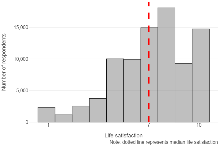
Median life satisfaction appears to be relatively high in the sample (7 out of 10)
med_satisfaction = np.median(wvs["satisfaction"])

(
  ggplot(wvs, aes("satisfaction")) +
  geom_histogram(fill = "grey", colour = "black", bins = 10, alpha = 0.5) +
  geom_vline(xintercept = med_satisfaction, linetype = "dashed", size = 2, colour = "red") +
  scale_x_continuous(breaks = [1, med_satisfaction, 10]) +
  theme_minimal() +
  theme(panel_grid_minor = element_blank(),
        panel_grid_major_x=element_blank()) +
  labs(x = "Life satisfaction", y = "Number of respondents",
       caption = "Note: dotted line represents median life satisfaction")
)
Life satisfaction tracks positively with financial situation
wvs_count = wvs.value_counts(["financial_situ", "satisfaction"]).reset_index()

(
  ggplot(wvs_count, aes("financial_situ", "satisfaction", size = "count")) +
  geom_point() +
  scale_x_continuous(breaks = np.arange(2, 12, 2)) +
  scale_y_continuous(breaks = np.arange(2, 12, 2)) +
  theme(panel_grid = element_blank(),
        panel_background = element_rect(fill = "white"),
        legend_position = "bottom") +
  labs(x = "Financial situation", y = "Life satisfaction")
)
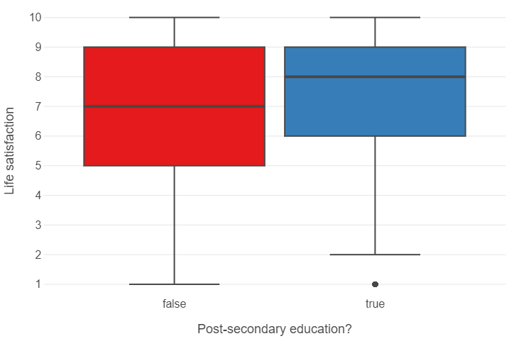
The median individual with post-secondary education has a higher life satisfaction than the median individual without
(
  ggplot(wvs, aes("post_second_edu", "satisfaction", fill = "post_second_edu")) +
  geom_boxplot() +
  theme_minimal() +
  theme(panel_grid_minor = element_blank(),
        panel_grid_major_x = element_blank(),
        legend_position="none") +
  labs(x = "Post-secondary education?", y = "Life satisfaction")
)
Understanding life satisfaction: the hypothesis-testing approach (5 minutes)
Why do some people have a higher life satisfaction than others? This is one question that a quantitative social scientist might answer by exploring the magnitude and precision of a series of variables. Suppose we hypothesised that individuals with post-secondary level education have greater life satisfaction relative to those who do not. We can estimate a linear regression model by using satisfaction as the dependent variable and post_second_edu as the independent variable.
To estimate a linear regression with interpretable output in Python, we can use the sm.OLS function, which requires two things:
- One or more features plus a constant
- An outcome
Let’s do this now. We can print the summary method to get information on the coefficient estimate for post_second_edu.
# Convert post_second_edu to float
X = wvs["post_second_edu"].astype(float)
# Add a constant
X = sm.add_constant(X)

# Isolate the feature column
y = wvs["satisfaction"]

# Build an OLS and print its output
model_univ = sm.OLS(y,X).fit()
print(model_univ.summary())

OLS Regression Results
==============================================================================
Dep. Variable:           satisfaction   R-squared:                       0.002
Model:                            OLS   Adj. R-squared:                  0.002
Method:                 Least Squares   F-statistic:                     160.6
Date:                Thu, 30 Jan 2025   Prob (F-statistic):           8.94e-37
Time:                        11:27:49   Log-Likelihood:            -1.9209e+05
No. Observations:               86867   AIC:                         3.842e+05
Df Residuals:                   86865   BIC:                         3.842e+05
Df Model:                           1
Covariance Type:            nonrobust
===================================================================================
                      coef    std err          t      P>|t|      [0.025      0.975]
-----------------------------------------------------------------------------------
const               7.0458      0.009    769.097      0.000       7.028       7.064
post_second_edu     0.2019      0.016     12.673      0.000       0.171       0.233
==============================================================================
Omnibus:                     5586.646   Durbin-Watson:                   1.674
Prob(Omnibus):                  0.000   Jarque-Bera (JB):             6736.238
Skew:                          -0.680   Prob(JB):                         0.00
Kurtosis:                       3.113   Cond. No.                         2.41
==============================================================================

Notes:
[1] Standard Errors assume that the covariance matrix of the errors is correctly specified.
We see that individuals with post-secondary education have a positive and statistically significant (p < 0.001) increase in life satisfaction of about 0.2 points.
👉 NOTE: The process of hypothesis testing is obviously more involved when using observational data than is portrayed by this simple example. Control variables will almost always be incorporated and, increasingly, identification strategies will be used to uncover causal effects. The end result, however, will involve as rigorous an attempt at falsifying a hypothesis as can be provided with the data.
For an example of how multivariate regression is used, we can run the following code.
# Create a function that normalises variables
def normalise(var):
  return (var-var.mean())/var.std()

# Create a data frame of features
X = wvs.drop(["satisfaction","iso3c"],axis=1)

# Identify which features are floats, categories and booleians
X_float = X.filter(items=["age","financial_situ","relig_import"],axis=1)
X_cat = X.filter(items=["employment","better_living"],axis=1)
X_bool = X[X.columns[~X.columns.isin(X_float+X_cat)]]

# Normalise numeric features
X_float = X_float.apply(lambda x: normalise(x),axis=0)

# Get dummies from categorical features
X_cat = pd.get_dummies(X_cat,drop_first=True, dtype=int)

# Convert booleian features to integers
X_bool = X_bool.astype(int)

# Concatenate to final data frame
X = pd.concat([X_float,X_cat,X_bool],axis=1)

# Add a constant
X = sm.add_constant(X)

# ISOLATING OUR OUTCOME
y = wvs["satisfaction"]
# BUILDING / SUMMARISING OUR MODEL
model_multiv = sm.OLS(y,X).fit()
print(model_multiv.summary())
OLS Regression Results
==============================================================================
Dep. Variable: satisfaction R-squared: 0.329
Model: OLS Adj. R-squared: 0.329
Method: Least Squares F-statistic: 1935.
Date: Thu, 30 Jan 2025 Prob (F-statistic): 0.00
Time: 11:28:12 Log-Likelihood: -1.7485e+05
No. Observations: 86867 AIC: 3.497e+05
Df Residuals: 86844 BIC: 3.500e+05
Df Model: 22
Covariance Type: nonrobust
=================================================================================================
coef std err t P>|t| [0.025 0.975]
-------------------------------------------------------------------------------------------------
const 7.1728 0.020 352.324 0.000 7.133 7.213
age -0.0006 0.008 -0.078 0.938 -0.016 0.015
financial_situ 1.1598 0.007 173.978 0.000 1.147 1.173
relig_import 0.1857 0.007 27.921 0.000 0.173 0.199
employment_House wife/husband 0.0012 0.022 0.055 0.956 -0.042 0.044
employment_Other 0.1059 0.058 1.811 0.070 -0.009 0.220
employment_Part time 0.1039 0.024 4.400 0.000 0.058 0.150
employment_Retired -0.0225 0.024 -0.932 0.351 -0.070 0.025
employment_Self employed -0.0107 0.020 -0.545 0.586 -0.049 0.028
employment_Student -0.0165 0.030 -0.543 0.587 -0.076 0.043
employment_Unemployed -0.1378 0.025 -5.450 0.000 -0.187 -0.088
better_living_Better off -0.0025 0.014 -0.174 0.862 -0.031 0.026
better_living_Worse off -0.4222 0.019 -21.932 0.000 -0.460 -0.384
social_trust 0.0733 0.015 4.839 0.000 0.044 0.103
male -0.0492 0.013 -3.705 0.000 -0.075 -0.023
post_second_edu -0.0335 0.014 -2.409 0.016 -0.061 -0.006
rural -0.0419 0.014 -3.039 0.002 -0.069 -0.015
married 0.1908 0.014 13.798 0.000 0.164 0.218
no_food -0.1663 0.021 -8.050 0.000 -0.207 -0.126
no_safety -0.0507 0.018 -2.783 0.005 -0.086 -0.015
no_medical -0.1286 0.018 -7.037 0.000 -0.164 -0.093
no_cash 0.0226 0.017 1.333 0.183 -0.011 0.056
no_shelter -0.2384 0.026 -9.214 0.000 -0.289 -0.188
==============================================================================
Omnibus: 3453.253 Durbin-Watson: 1.818
Prob(Omnibus): 0.000 Jarque-Bera (JB): 8250.356
Skew: -0.228 Prob(JB): 0.00
Kurtosis: 4.439 Cond. No. 15.5
==============================================================================
Notes:
[1] Standard Errors assume that the covariance matrix of the errors is correctly specified.Interestingly, we can see that the coefficient estimate for post_second_edu is now negative and significant, albeit at a lower level than before (p < 0.05).
👉 NOTE: p-values are useful to machine learning scientists as they indicate which variables may yield a significant increase in model performance. However, p-hacking where researchers manipulate data to find results that support their hypothesis make it hard to tell whether or not a relationship held up after honest attempts at falsification. This can range from using a specific modelling approach that produces statistically significant (while failing to report others that do not) findings to outright manipulation of the data. For a recent egregious case of the latter, we recommend the Data Falsificada series.
Predicting life satisfaction: the machine learning approach (30 minutes)
Machine learning scientists take a different approach. Our aim, in this context, is to build a model that can be used to accurately predict how happy a person is using a mixture of features and, for some models, hyperparameters (which we will address in Lab 5).
Thus, rather than attempting to falsify the effects of causes, we are more concerned about the fit of the model in the aggregate when applied to unforeseen data.
To achieve this, we do the following:
- Split the data into training and test sets
- Build a model using the training set
- Evaluate the model on the test set
Let’s look at each of these in turn.
Split the data into training and test sets
It is worth considering what a training and test set is and why we might split the data this way.
A training set is data that we use to build (or “train”) a model. In the case of multivariate linear regression, we are using the training data to estimate a series of coefficients. Here is a made-up multivariate linear model with three coefficients derived from (non-existent) data to illustrate things.
def sim_model_preds(x1,x2,x3):
  y = 1.1*x1 + 2.2*x2 + 3.3*x3
  return y
A test set is data that the model has not yet seen. We then apply the model to this data set and use an evaluation metric to find out how accurate our predictions are. For example, suppose we had a new observation where x1 = 10, x2 = 20 and x3 = 30 and y = 150. We can use the above model to develop a prediction.
sim_model_preds(10,20,30)

154.0
We get a prediction of 154 points!
We can also calculate the amount of error we make by calculating residuals (actual value - predicted value).
150 - sim_model_preds(10, 20, 30)

-4.0
We can see that our model is 4 points off the real answer!
Why do we evaluate our models using different data? Because, as stated earlier, machine learning scientists care about the applicability of a model to unforeseen data. If we were to evaluate the model using the training data, we obviously cannot do this to begin with. Furthermore, we cannot ascertain whether the model we have built can generalise to other data sets or if the model has simply learned the idiosyncrasies of the data it was used to train on. We will discuss the concept of overfitting throughout this course.
We can use train_test_split in sklearn.model_selection to split the data into training and test sets.
X_train, X_test, y_train, y_test = train_test_split(X, y, random_state = 123)👉 NOTE: Our data are purely cross-sectional, so we can use this approach. However, when working with more complex data structures (e.g. time series cross sectional), different approaches to splitting the data will need to be used.
Build a model using the training set
We will now switch our focus from statsmodels to scikit-learn, the latter being Python’s most comprehensive and popular machine learning library.
Below, we will see how simple it is to run a model in this library. We have done all the data cleaning needed, so we can just get to it!
# Create a model instance of a linear regression
linear_model = LinearRegression()

# Fit this instance to the training set
linear_model.fit(X_train, y_train)
Evaluate the model using the test set
Now that we have trained a model, we can then evaluate its performance on the test set. We will look at two evaluation metrics:
- R-squared: the proportion of variance in the outcome explained by the model.
- Root mean squared error (RMSE): the amount of error a typical observation parameterised as the units used in the initial measurement.
# Create predictions for the test set
linear_preds = linear_model.predict(X_test)

# Calculate performance metrics
r2 = r2_score(y_test, linear_preds)
rmse = root_mean_squared_error(y_test, linear_preds)

# Print results
print(np.round(r2, 2), np.round(rmse, 2))

0.33 1.81
🗣️ CLASSROOM DISCUSSION:
How can we interpret these results?
We find that the model explains ~ 33% of the test set variance in life satisfaction. We also find that our model predictions are off by ~ 1.8 points.
Graphically exploring where we make errors
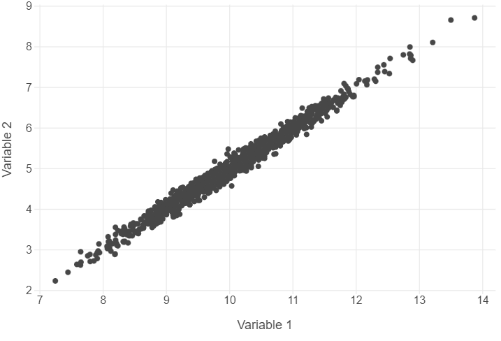
We are going to build some residual scatter plots which look at the relationship between the values fitted by the model for each observation and the residuals (actual - predicted values). Before we do this for our data, let’s take a look at an example where there is a near perfect relationship between two variables. As this very rarely exists in the social world, we will rely upon simulated data.
We translated and adapted this code from here.
# Set a seed for reproducibility
np.random.seed(123)

# Create the variance covariance matrix
sigma = [[1,0.99],[0.99,1]]

# Create the mean vector
mu = [10,5]

# Generate a multivariate normal distribution using 1,000 samples
v1, v2 = np.random.multivariate_normal(mu,sigma,1000).T

# Combine to a data frame
sim_data = pd.DataFrame({"V1":v1,"V2":v2})
Plot the correlation
(
  ggplot(sim_data, aes("V1", "V2")) +
  geom_point() +
  theme_minimal() +
  theme(panel_grid_minor = element_blank()) +
  labs(x = "Variable 1", y = "Variable 2")
)
Residual plots
# Build a linear model
sim_fit = linear_model.fit(v1.reshape(-1,1),v2.reshape(-1,1))
sim_preds = linear_model.predict(v1.reshape(-1,1))

# Combine predictions / residuals to a data frame
sim_residuals_toplot = pd.DataFrame({"predictions": sim_preds.reshape(-1),
                                     "residuals": v2 - sim_preds.reshape(-1)})

# Plot the results
(
  ggplot(sim_residuals_toplot, aes("predictions", "residuals")) +
  geom_hline(yintercept = 0, linetype = "dashed") +
  geom_point() +
  theme_minimal() +
  theme(panel_grid_minor = element_blank()) +
  scale_y_continuous(limits=[-7,7]) +
  labs(x = "Fitted values", y = "Residuals")
)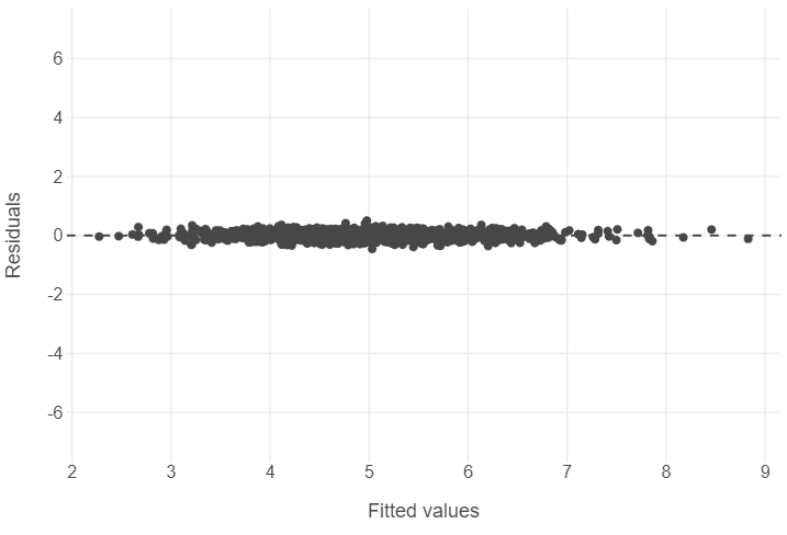
Now let’s run this code for our model.
residuals_toplot = pd.DataFrame({"predictions": linear_preds,
                                 "residuals": np.array(y_test) - linear_preds})
(
  ggplot(residuals_toplot, aes("predictions", "residuals")) +
  geom_hline(yintercept = 0, linetype = "dashed") +
  geom_point() +
  theme(panel_grid_minor = element_blank()) +
  labs(x = "Fitted values", y = "Residuals")
)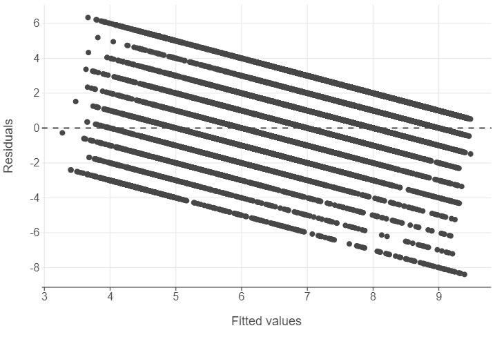
🎯 ACTION POINTS why does the graph of the simulated data illustrate a more well-fitting model when compared to our actual data?
The spread of our values in the actual data is relatively large. Furthermore, we see that as our fitted values become larger, we go from underpredicting to overpredicting life satisfaction.
Introduction to using list comprehensions to aid feature selection (30 minutes)
👨🏻🏫 TEACHING MOMENT: Your tutor will take you through the code, so sit back, relax and enjoy!
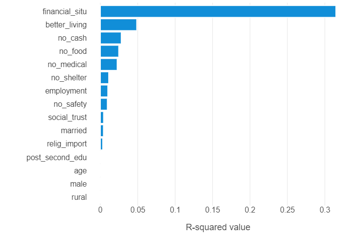
Remember our univariate model earlier? We are going to do the same for all features so see which ones show the best improvements in predictive power.
We could build 15 different model objects, but this would be very inefficient. Instead, we are going to build a function that calculates the \(R2\) for a given feature and apply it to all features using a list comprehension.
Create a list of feature names
feature_names = wvs.drop(["iso3c","satisfaction"],axis=1).columnsDefine a function to get r-squared values for each feature
This gets a little tricky! Remember that we have transformed all our categorical features into one-hot encoded dummy variables. We need to therefore make sure that all dummies in one feature are included. The trick we’ve opted for is to use our original feature names to loop over. In the get_r2 we use a logical condition X_train.columns.str.contains(feature) which simply asks “does a given column name contain the string value of a given feature?”
def get_r2(feature):
  """

  Runs a linear model using a subset of features in a training set and calculates
  the r-squared for each model, using a test set. The output is a single value.

  """

  # Create subsetted data
  train = X_train[X_train.columns[X_train.columns.str.contains(feature)]]
  test = X_test[X_test.columns[X_test.columns.str.contains(feature)]]

  # Instantiate and run a linear model on subsetted data
  linear_model = LinearRegression()
  linear_model.fit(train,y_train)

  # Create the predictions
  preds = linear_model.predict(test)

  # Calculate r-squared
  r2 = r2_score(y_test,preds)
  return r2
We can check to see the function works by trying it on a feature or two. Let’s try this for financial situation.
get_r2("financial_situ")

0.3147842601900087
Use a list comprehension to loop get_r2 over all features
r2s = [get_r2(feat) for feat in feature_names]Create a data frame showing the r-squared for each feature
linear_output = pd.DataFrame({"feature":feature_names,"r2":r2s})
linear_output = linear_output.sort_values(by = "r2")
Plot the results!
(
  ggplot(linear_output, aes("r2", "feature")) +
  geom_bar(stat = "identity") +
  theme_minimal() +
  theme(panel_grid_minor = element_blank(),
        panel_grid_major_y = element_blank()) +
  labs(x = "R-squared value", y = "")
)
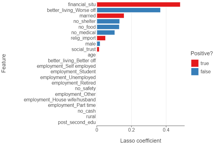
Using penalised linear regression to perform feature selection (20 minutes)
We are now going to experiment with a lasso regression which, in this case, is a linear regression that uses a so-called hyperparameter - a “dial” built into a given model that can be experimented with to improve model performance. The hyperparameter in this case is a regularisation penalty which takes the value of a non-negative number. This penalty can shrink the magnitude of coefficients down to zero and the larger the penalty, the more shrinkage occurs.
Step 1: Create a lasso model
Run the following code. This builds a lasso model with the penalty parameter set to 0.01.
lasso_model = Lasso(alpha = 0.01)
lasso_model.fit(X_train, y_train)
Step 2: Extract lasso coefficients
# Create a data frame with feature columns and Lasso coefficients
lasso_output = pd.DataFrame({"feature": X_train.columns, "coefficient": lasso_model.coef_})

# Code a positive / negative vector
lasso_output["positive"] = np.where(lasso_output["coefficient"] >= 0, True, False)

# Take the absolute value of the coefficients
lasso_output["coefficient"] = np.abs(lasso_output["coefficient"])

# Remove the constant and sort the data frame by (absolute) coefficient magnitude
lasso_output = lasso_output.query("feature != 'const'").sort_values("coefficient")
🎯 ACTION POINTS What is the output? Which coefficients have been shrunk to zero? What is the most important feature?
The output is
lasso_output

    feature coefficient positive
1     age   0.000000    True
19  no_safety   0.000000    True
16  rural   0.000000    True
15  post_second_edu 0.000000    True
14  male    0.000000    True
21  no_cash 0.000000    True
9     employment_Student    0.000000    True
11  better_living_Better off    0.000000    True
7     employment_Retired    0.000000    True
5     employment_Other  0.000000    True
4     employment_House wife/husband 0.000000    True
8   employment_Self employed    0.000000    True
13  social_trust    0.006864    True
22  no_shelter  0.054865    False
10  employment_Unemployed   0.065437    False
6     employment_Part time  0.085227    True
20  no_medical  0.118321    False
17  married 0.142701    True
3     relig_import  0.176989    True
18  no_food 0.188848    False
12  better_living_Worse off 0.366195    False
2     financial_situ    1.171107    True
financial_situ is the most important feature (just as previously). The coefficients for age,no_safety,rural,post_second_edu,male,no_cash,employment_Student,better_living_Better off,employment_Retired,employment_Other,employment_House wife/husband and employment_Self employed have all been shrunk to 0
Step 3: Create a bar plot
(
  ggplot(lasso_output, aes("coefficient", "feature", fill = "positive")) +
  geom_bar(stat = "identity") +
  theme(panel_grid_major_y = element_blank()) +
  labs(x = "Lasso coefficient", y = "Feature",
       fill = "Positive?")
)
Step 4: Evaluate on the test set
Although a different model is used, the code for evaluating the model on the test set is exactly the same as earlier.
# Apply model to test set
lasso_preds = lasso_model.predict(X_test)

# Calculate performance metrics
lasso_r2 = r2_score(y_test, lasso_preds)
lasso_rmse = root_mean_squared_error(y_test, lasso_preds)

# Print rounded PMs
print(np.round(lasso_r2,2), np.round(lasso_rmse,2))

0.33 1.81
🗣️ CLASSROOM DISCUSSION:
What feature is the largest positive / negative predictor of life satisfaction? Does this model represent an improvement on the linear model?
No, we find more or less identical results to the linear model.
(Bonus) Step 5: Experiment with different penalties
This is your chance to try out different penalties. Can you find a penalty that improves test set performance?
Let’s try a lower penalty value of 0.001.
# Instantiate a lasso model
lasso_model = Lasso(alpha=0.001)

# Fit the model to the training data
lasso_model.fit(X_train, y_train)

# Apply the model to the test set
lasso_preds = lasso_model.predict(X_test)

# Calculate performance metrics
lasso_r2 = r2_score(y_test, lasso_preds)
lasso_rmse = root_mean_squared_error(y_test, lasso_preds)

# Print the rounded metrics
print(np.round(lasso_r2, 2), np.round(lasso_rmse, 2))

0.33 1.81
It looks like a penalty of 0.01 works just as well as a lower penalty.
👉 NOTE: In labs 4 and 5, we are going to use a method called k-fold cross validation to systematically test different combinations of hyperparameters for models such as the lasso.