LSE DS202W 2025: Week 4 - Lab Solutions

2024/25 Winter Term

Author

The DS202 Team

Published

10 Feb 2025

This solution file follows the format of a Jupyter Notebook file .ipynb you had to fill in during the lab session.

⚙️ Setup

Downloading the student solutions

Click on the below button to download the student notebook.

Loading libraries and functions

import numpy as np
import pandas as pd
from sklearn.model_selection import train_test_split
from sklearn.linear_model import LogisticRegression
from sklearn.linear_model import Lasso
from sklearn.metrics import precision_score, recall_score, f1_score, root_mean_squared_error
import statsmodels.api as sm
from lets_plot import *
LetsPlot.setup_html()

📋 Lab Tasks

Part I - Cleaning a new data set `monitor` (30 min)

The first step is to load the dataset. In this lab, we will be using the 2020 Wellcome Trust Global Monitor (monitor) dataset which contains data. It includes variables associated with trust in various actors and demographic information:

science_decreases_jobs: binary outcome where respondents are asked whether they believe science and technology will decrease (versus increase, or have no impact on) the amount of jobs available.
trust_neighbours: Trust People in Neighbourhood
trust_government: Trust the National Government in This Country
trust_scientists: Trust Scientists in This Country
trust_journalists: Trust Journalists in This Country
trust_doctors: Trust Doctors and Nurses in This Country
trust_ngos: Trust People Who Work at Charitable Organizations or NGOs in This Country
trust_trad_healers: Trust Traditional Healers in This Country
age: Age (years)
gender: Male / Female
education: Education Level (Elementary / Secondary / Tertiary)
hh_income: Per Capita Income Quintiles
subj_income: Feelings About Household Income
emp_status: Employment Status

👉 NOTE: With variables such as trust_neighbours, we recoded the original question to a trust / no trust binary mainly for the sake of simplicity. This simplification can be useful as it reduces the number of parameters in our model. However, there may be distinct differences between each level that may produce different results.

monitor = pd.read_csv("data/wellcome_global_monitor.csv")

📝Task: Check the dimensions of the dataframe.

print(monitor.shape)

(119088, 14)

📝Task: Here’s another check we can perform quickly in pandas. If we use the isnull method and then calculate the mean, we can check the proportion of missing values contained within each variable.

print(monitor.isnull().mean())

science_decreases_jobs    0.0
trust_neighbours          0.0
trust_government          0.0
trust_scientists          0.0
trust_journalists         0.0
trust_doctors             0.0
trust_ngos                0.0
trust_trad_healers        0.0
age                       0.0
gender                    0.0
education                 0.0
hh_income                 0.0
subj_income               0.0
emp_status                0.0
dtype: float64

📝Task: We need to perform some variable transformations. Normalise age, convert all logical variables to integer variables (check out astype), and code all categorical features as one-hot encoded dummies.

# Create a function that normalises variables
def normalise(var):
  return (var-var.mean())/var.std()

# Identify column types
logical_vars = monitor.columns[monitor.columns.str.contains("trust")]
categorical_vars = ["gender","education", "hh_income", "subj_income", "emp_status"]

# Perform cleaning
monitor_cleaned = monitor
monitor_cleaned[logical_vars] = monitor_cleaned[logical_vars].astype(int)
monitor_cleaned["age"] = normalise(monitor_cleaned["age"])
monitor_cleaned = pd.get_dummies(monitor_cleaned,columns=categorical_vars,drop_first=True,dtype=int)

📝Task: How many observations fall into each class of the variable science_decreases_jobs? Comment. What are the challenges you would expect when training a model?

monitor_cleaned.value_counts("science_decreases_jobs")

science_decreases_jobs
False    83077
True     36011
Name: count, dtype: int64

Our dataset is imbalanced: there are many more individuals who believe that science and technology will not take their jobs (class 0) than individuals who do (class 1).

📝Task: Come up with one or two summary visualisations!

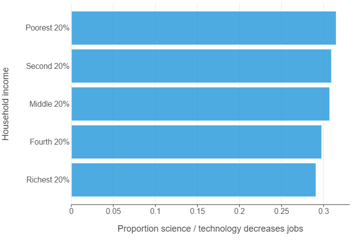
The gap between rich and poor regarding science / technology taking jobs is quite small!

reorder_hh = {"Poorest 20%":4,"Second 20%":3,"Middle 20%":2,
              "Fourth 20%":1,"Richest 20%":0}

monitor_summary = monitor.\
    filter(items=["science_decreases_jobs","hh_income"]).\
    groupby("hh_income",as_index=False).\
    mean().\
    sort_values(by=["hh_income"], key=lambda x: x.map(reorder_hh))

(
    ggplot(monitor_summary, aes("science_decreases_jobs", "hh_income")) +
    geom_bar(stat="identity", alpha = 0.75) +
    theme(panel_grid_major_y=element_blank()) +
    labs(x = "Proportion science / technology decreases jobs", y = "Household income")
)

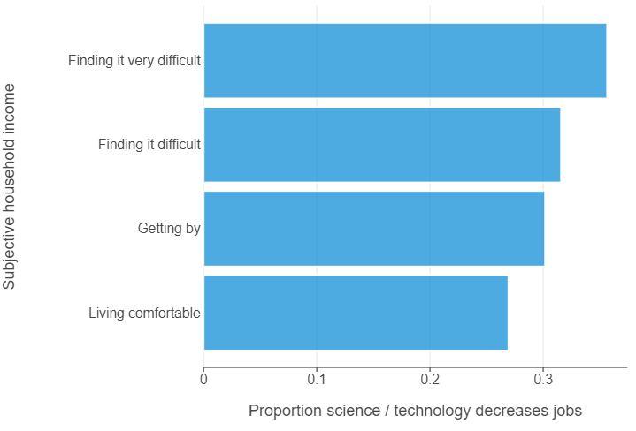
The same gap between the economically insecure and secure is much larger!

reorder_subj = {"Living comfortable on present income":0,
                "Getting by on present income":1,
                "Finding it difficult on present income":2,
                "Finding it very difficult on present income":3}

monitor_summary = monitor.\
    filter(items=["science_decreases_jobs","subj_income"]).\
    groupby("subj_income",as_index=False).\
    mean().\
    sort_values(by=["subj_income"], key=lambda x: x.map(reorder_subj))

monitor_summary["subj_income"] = monitor_summary["subj_income"].str.replace(" on present income", "")

(
    ggplot(monitor_summary, aes("science_decreases_jobs", "subj_income")) +
    geom_bar(stat="identity", alpha = 0.75) +
    theme(panel_grid_major_y=element_blank()) +
    labs(x = "Proportion science / technology decreases jobs", y = "Subjective household income")
)

Part II - Fitting a logistic regression (40 min)

We want to perform a logistic regression using the available variables in the dataset to predict whether an individual thinks that science will decrease jobs.

👨🏻‍🏫 TEACHING MOMENT: Your class teacher will formalize the logistic regression in the context of the data at our disposal.

Now, we need to split the data into training and testing sets. Having a test set will help us evaluate how well the model performs.

In the training phase, we will use part of the data to fit the logistic regression model.
In the testing phase, we will assess the model’s performance on the remaining data (test set) which was not used during training.

# Divide data into features (X) and targets (y) 
X = monitor_cleaned.drop("science_decreases_jobs", axis=1).astype(float)
X = sm.add_constant(X)
y = monitor_cleaned["science_decreases_jobs"].astype(int)

# Perform a 0.75 / 0.25 train / test
X_train, X_test, y_train, y_test = train_test_split(X, y, stratify=y, random_state=123)

💡Tip: When using train_test_split try specifying stratify = y. This ensures that the training and test sets will have identical proportions of the outcome.

We will now fit a logistic regression model on the training data using statsmodels.

logit_model = sm.Logit(y_train, X_train).fit()
print(logit_model.summary())

Optimization terminated successfully.
         Current function value: 0.595142
         Iterations 5
                             Logit Regression Results                             
==================================================================================
Dep. Variable:     science_decreases_jobs   No. Observations:                89316
Model:                              Logit   Df Residuals:                    89292
Method:                               MLE   Df Model:                           23
Date:                    Thu, 06 Feb 2025   Pseudo R-squ.:                 0.02893
Time:                            09:32:51   Log-Likelihood:                -53156.
converged:                           True   LL-Null:                       -54739.
Covariance Type:                nonrobust   LLR p-value:                     0.000
===========================================================================================================================
                                                              coef    std err          z      P>|z|      [0.025      0.975]
---------------------------------------------------------------------------------------------------------------------------
const                                                      -0.2195      0.039     -5.562      0.000      -0.297      -0.142
trust_neighbours                                           -0.0367      0.018     -2.009      0.045      -0.073      -0.001
trust_government                                           -0.4455      0.016    -27.654      0.000      -0.477      -0.414
trust_scientists                                           -0.1670      0.021     -8.057      0.000      -0.208      -0.126
trust_journalists                                          -0.2412      0.016    -14.794      0.000      -0.273      -0.209
trust_doctors                                              -0.1147      0.022     -5.187      0.000      -0.158      -0.071
trust_ngos                                                 -0.1490      0.017     -8.543      0.000      -0.183      -0.115
trust_trad_healers                                         -0.0869      0.015     -5.654      0.000      -0.117      -0.057
age                                                         0.1614      0.008     20.614      0.000       0.146       0.177
gender_Male                                                -0.0193      0.015     -1.267      0.205      -0.049       0.011
education_Secondary (8-15 years)                            0.3059      0.024     12.690      0.000       0.259       0.353
education_Tertiary                                          0.2953      0.027     11.105      0.000       0.243       0.347
hh_income_Middle 20%                                        0.0646      0.023      2.762      0.006       0.019       0.110
hh_income_Poorest 20%                                       0.0757      0.026      2.954      0.003       0.025       0.126
hh_income_Richest 20%                                      -0.0322      0.022     -1.490      0.136      -0.075       0.010
hh_income_Second 20%                                        0.0479      0.025      1.953      0.051      -0.000       0.096
subj_income_Finding it very difficult on present income     0.1362      0.027      5.052      0.000       0.083       0.189
subj_income_Getting by on present income                   -0.0414      0.021     -2.013      0.044      -0.082      -0.001
subj_income_Living comfortable on present income           -0.1643      0.024     -6.957      0.000      -0.211      -0.118
emp_status_Employed full time for self                     -0.1293      0.025     -5.274      0.000      -0.177      -0.081
emp_status_Employed part time do not want full time        -0.0133      0.033     -0.408      0.684      -0.077       0.051
emp_status_Employed part time want full time               -0.0833      0.029     -2.859      0.004      -0.140      -0.026
emp_status_Out of workforce                                -0.0545      0.020     -2.786      0.005      -0.093      -0.016
emp_status_Unemployed                                       0.0275      0.031      0.878      0.380      -0.034       0.089
===========================================================================================================================

👨🏻‍🏫 TEACHING MOMENT: Your class teacher will explain how to interpret the summary of the model (\(p-\)values, AIC …).

We can run the same model using scikit-learn by specifying the following code.

# Instantiate / fit a logistic regression model
logit_model = LogisticRegression() 
logit_model.fit(X_train, y_train)

Next, we will generate predicted probabilities on both the training and testing sets from our logistic regression model using predict_proba.

# Generate predictions on the training set
train_probas = logit_model.predict_proba(X_train)[:,1]

# Generate predictions on the testing set
test_probas = logit_model.predict_proba(X_test)[:,1]

💡Tip: predict_proba produces a 2-d numpy array which predicts the probability of the outcome not occurring (the 1st dimension) and occurring (the 2nd dimension). To select the 2nd dimension (and all the rows), employ this indexing [:,1] when using this function.

test_probas[0:10]

array([0.26031154, 0.35727596, 0.46766817, 0.33238068, 0.22080559,
       0.29925601, 0.28789836, 0.42926639, 0.36675032, 0.32610668])

We are going to set an arbitrary threshold \(\alpha\). All the scores that are higher than \(\alpha=0.6\) will be classified as 1 and the scores lower than \(\alpha=0.6\) will be classified as 0.

# Convert predicted scores to binary outcomes for the training set
train_preds = np.where(train_probas > 0.6, 1, 0)

# Convert predicted scores to binary outcomes for the testing set
test_preds = np.where(test_probas > 0.6, 1, 0)

👨🏻‍🏫 TEACHING MOMENT: Your class teacher will explain what precision and recall are.

Now, let’s print the precision and recall for both training and testing sets.

print(f"Training set precision: {np.round(precision_score(y_train, train_preds), 3)}")
print(f"Testing set precision: {np.round(precision_score(y_test, test_preds), 3)}")
print(f"Training set recall: {np.round(recall_score(y_train, train_preds), 3)}")
print(f"Testing set recall: {np.round(recall_score(y_test, test_preds), 3)}")

Training set precision: 0.477
Testing set precision: 0.467
Training set recall: 0.001
Testing set recall: 0.001

❓Question: Compare the results you obtain for both the training and testing sets. Was this expected ? Does the model overfit ? underfit ?

We find that precision is reduced by 1 percentage point. Recall is uniformly poor.

❓Question: What is the problem with setting an arbitrary threshold \(\alpha=0.6\) ? How should we expect the precision and the recall to behave if we increase the threshold \(\alpha\) ? If we decrease \(\alpha\) ?

First of all, we need to consider how balanced our data are between different classes in the outcome. If we plot the distribution of predictions of belief in science/technology taking jobs, for example, very few observations have a probability of above 0.5, let alone 0.6! This will result in recall being very low. However, setting the threshold too low will result in reduced precision as more individuals with a low probability of believing in science/technology taking jobs will nevertheless be classified as such.

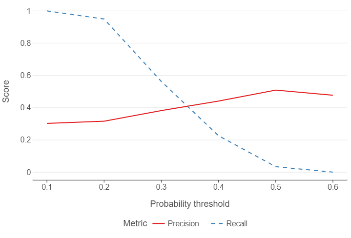
We will now compute the precision and recall for the test set for different values of the threshold \(\alpha\). Compute them for \(\alpha \in \{0.1, 0.2, 0.3, 0.4, 0.5, 0.6 \}\).

th_list = np.arange(0.1, 0.7, 0.1)

def test_proba_th(th, prob_est, truth):
  class_preds = np.where(prob_est > th, 1, 0)
  prec = precision_score(truth, class_preds)
  sens = recall_score(truth, class_preds)
  return prec, sens

metrics = [test_proba_th(th,train_probas,y_train) for th in th_list]

output = pd.DataFrame({"threshold": th_list, 
                       "Precision": [m[0] for m in metrics],
                       "Recall": [m[1] for m in metrics]})

print(output)

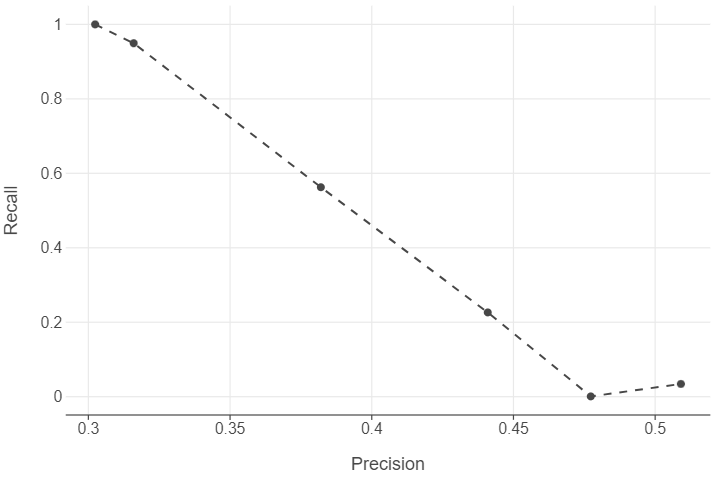
threshold  Precision    Recall
0        0.1   0.302387  1.000000
1        0.2   0.315991  0.949459
2        0.3   0.382039  0.562648
3        0.4   0.440926  0.226340
4        0.5   0.509091  0.034212
5        0.6   0.477273  0.000778

👨🏻‍🏫 TEACHING MOMENT: Your teacher will explain what the code chunk is doing.

We specify a probability threshold range using np.arange. Note, when we specify an interval of 0.1, we need to set the maximum value to 0.7 to get 0.6.
We build a function using np.where that creates a binary variable depending on the probability threshold selected and then calculates precision / recall scores.
We loop the function over the different thresholds using list comprehension.
We create a data frame with the thresholds and precision and recall scores. While we have a list of thresholds, we need to use list comprehension to get the correct dimension of metrics, which is a 2-d numpy array.

Let’s create a plot that shows performance over different thresholds, using colour to distinguish between the different evaluation metrics.

output_melted = pd.melt(output, id_vars="threshold")

(
  ggplot(output_melted, aes("threshold", "value", colour = "variable", linetype = "variable")) +
  geom_line() +
  theme(panel_grid_minor = element_blank(),
        panel_grid_major_x = element_blank(),
        legend_position = "bottom") +
  labs(x = "Probability threshold", y = "Score", colour = "Metric", linetype = "Metric")
)

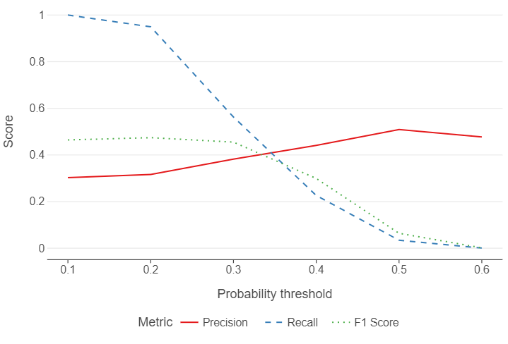
📝Task: Try redefining class_metrics to also include f1_score and see what happens.

def test_proba_th(th, prob_est, truth):
  class_preds = np.where(prob_est > th, 1, 0)
  prec = precision_score(truth, class_preds)
  sens = recall_score(truth, class_preds)
  f1 = f1_score(truth, class_preds)
  return prec, sens, f1

metrics = [test_proba_th(th, train_probas, y_train) for th in th_list]

output = pd.DataFrame({"threshold": th_list, 
                       "Precision": [m[0] for m in metrics],
                       "Recall": [m[1] for m in metrics],
                       "F1 Score": [m[2] for m in metrics]})

output_melted = pd.melt(output, id_vars="threshold")

(
  ggplot(output_melted, aes("threshold", "value", colour = "variable", linetype = "variable")) +
  geom_line() +
  theme(panel_grid_minor = element_blank(),
        panel_grid_major_x = element_blank(),
        legend_position = "bottom") +
  labs(x = "Probability threshold", y = "Score", colour = "Metric", linetype = "Metric")
)

📝Task: Based on the precision and recall values you calculated, create a precision-recall plot to visualize the relationship between these two metrics. How does the shape of the precision-recall curve help you assess model performance ? What trade-offs do you observe between precision and recall ?

We see that generally, there is a precision-recall trade off.

(
  ggplot(output, aes("Precision", "Recall")) +
  geom_point() +
  geom_line(linetype = "dashed") 
)

Working with time-series cross-sectional data in machine learning (30 mins)

Economists and political scientists constantly work with data that has a cross-sectional (e.g. between country) and time-series (e.g. within countries over years) structure. This poses an interesting challenge for when we perform a train / test split. If we use train_test_split on such data, the function will assume that it is cross-sectional and perform an initial split without taking the time-series dimension into account. In doing so, we run the risk of:

Using future values to predict the past
Using information from the same country in the training and testing sets

Naturally, a few solutions follow from this issue:

Use earlier years to train the model and later years to test it.
Use some countries to train the model and other countries to test it.

📝Task: Use GDP per capita in the Gapminder data set (see the Week 2 lab) to predict life expectancy.

Open the data set.

gapminder = pd.read_csv("data/gapminder.csv")

Convert the variable names to snake case (see Lab 2).

# Create a dictionary of variable names using snake case
snake_case_var_names = {
  "country":"country",
  "continent":"continent",
  "year":"year",
  "lifeExp": "life_exp",
  "pop":"pop",
  "gdpPercap":"gdp_per_cap"
}

# Set the columns attribute to this list
gapminder = gapminder.rename(columns=snake_case_var_names)

Splitting the data by year

Use data from 2007 as the testing data, and all other years as the training data.

train, test = gapminder.query("year < 2007"), gapminder.query("year == 2007")

Split the training / testing data into outcomes and features (remember to convert the series into a one-column data frame).

X_train, X_test = train["gdp_per_cap"].to_frame(), test["gdp_per_cap"].to_frame()
y_train, y_test = train["life_exp"].to_frame(), test["life_exp"].to_frame()

Build a linear model on the training set, and evaluate it on the test set, using RMSE

# Instantiate a lasso model
lasso_model = Lasso(alpha=0.01)

# Fit the model on the training set
lasso_model.fit(X_train, y_train)

# Create predictions for the test set
preds = lasso_model.predict(X_test)

# Calculate RMSE
rmse = root_mean_squared_error(y_test, preds)

# Summarise the results
print(f"On average, our model is approximately {np.round(rmse, 2)} years off!")

On average, our model is approximately 10.05 years off!

Splitting the data by country

Create an array of all unique country values.

countries = gapminder["country"].unique()

Randomly sample 36 countries (~25% of all countries in gapminder) to be in the test set.

💁Tip: You’ll need a couple of functions from numpy.random first, to set a random seed (seed) for reproduceability and, second, to select the number of countries (choice).

from numpy.random import seed, choice

seed(123)
test_countries = choice(countries, size=36)

Split the data into training and testing sets.

train = gapminder.query("country not in @test_countries")
test = gapminder.query("country in @test_countries")