
Week 07 - Lab Solutions
Dimensionality reduction using PCA and UMAP
This solution file follows the format of a Jupyter Notebook file .ipynb you had to fill in during the lab session.
⚙️ Setup
Downloading the student solutions
Click on the below button to download the student notebook.
Loading libraries
import numpy as np
import pandas as pd
from sklearn.decomposition import PCA
from sklearn.pipeline import Pipeline
from sklearn.preprocessing import StandardScaler
from umap import UMAP
import plotly.express as px
from lets_plot import *
LetsPlot.setup_html()
🥅 Learning Objectives
By the end of this lab, you will be able to:
- Understand the concept of dimensionality reduction
- Apply principal component analysis (PCA) to perform dimensionality reduction
- Apply Uniform Manifold Approximation and Projection (UMAP) to perform dimensionality reduction
Exploring ethical values and norms in the World Values Survey (15 minutes)
The WVS provides information on 19 such issues which respondents can rate from 0 (never justifiable) to 10 (always justifiable), including:
Q177: Claiming government benefits to which you are not entitledQ178: Avoiding a fare on public transportQ179: Stealing propertyQ180: Cheating on taxes if you have a chanceQ181: Someone accepting a bribe in the course of their dutiesQ182: HomosexualityQ183: ProstitutionQ184: AbortionQ185: DivorceQ186: Sex before marriageQ187: SuicideQ188: EuthanasiaQ189: For a man to beat his wifeQ190: Parents beating childrenQ191: Violence against other peopleQ192: Terrorism as a political, ideological or religious meanQ193: Having casual sexQ194: Political violenceQ195: Death penalty
🗣️ CLASSROOM DISCUSSION: How could we explore relationships between these features?
We could look at scatter plots between all pairs of variables. But remembering relationships between all pairs would be cumbersome.
🎯 ACTION POINT: Read the data set into Python (set low_memory = False)
wvs = pd.read_csv("../data/wvs-wave-7-ethical-norms.csv", low_memory=False)🎯 ACTION POINT: Rename the variables to better reflect the ethical value / norm
# Create a list of columns to keep
keys = [f"Q{i}" for i in range(177,196)]

# Create a list of descriptive labels for the columns
values = ["cheating_benefits","avoid_transport_fare","stealing_property",
          "cheating_taxes","accept_bribes","homosexuality","sex_work",
          "abortion","divorce","sex_before_marriage","suicide","euthanasia",
          "violence_against_spouse","violence_against_child","social_violence","terrorism",
          "casual_sex","political_violence","death_penalty"]

# Create a dictionary to rename the columns in the data frame
vars_renamed = dict(zip(keys,values))

# Employ the changes to data frame
wvs_cleaned = wvs.rename(columns=vars_renamed)
Principle Component Analysis with the World Values Survey (45 minutes)
Besides making data exploration and visualization difficult, high dimensional data comes with other challenges too, in particular with regards to supervised learning.
🧑🏫 TEACHING MOMENT:
The Curse of Dimensionality 🪄
No, that’s not a Harry Potter spell but it refers to the problems that often arise when dealing with high dimensional data (ie lots of variables).
Machine learning models tend to perform badly with too many features - there is a higher chance for overfitting, plus there is also a much bigger computational cost associated to training models with many variables.
Dimensionality Reduction to the Rescue 🧑⚕️
We want to reduce the number of variables. Intuitively, this could work because there are often strong correlations between many of the individual variables. In other words, there is redundancy in the data.
Dimensionality reduction refers to a collection of methods that can help reduce the number of variables while preserving most of the information. PCA is one such method.
Principal Component Analysis (PCA) 💡
However, rather than deciding which variables to keep and which ones to throw out (that would fall under “variable selection”), we want to compress our high dimensional data into a low dimensional set of variables while retaining as much information from the original data as possible.
To implement PCA, we must first normalise our variables. Up until now, we have employed a user-based function. However, because we have only numeric features, we can actually perform the data transformation and PCA in one step using pipelines! Pipeline consists of a list of tuples, (user defined step name, model instantiation) that can be seen as a series of steps to be run in order to apply a model.
🎯 ACTION POINT: Use Pipeline to combine StandardScaler() and PCA() and fit the pipeline to the cleaned data.
# Create a pipeline whereby all features are scaled
pipe = Pipeline([("scaler", StandardScaler()), ("pca", PCA())])

# Fit the pipeline to the full data set
_ = pipe.fit(wvs_cleaned.values)
🎯 ACTION POINT: With pipelines, accessing the attributes of each step may seem tricky at first. Luckily, however, any pipeline has a named_steps attribute, which can allow you to explore all the attributes that pertain to a specific step. Try this with the explained_variance_ratio_ attribute which gives us the proportion of variance explained by each principle component between all features. Ideally, we would like to see a graph showing the cumulative proportion of variance explained over the first 10 principle components.
# Getting the array is simple enough
print(pipe.named_steps["pca"].explained_variance_ratio_)

[0.34317401 0.17419084 0.06569919 0.04997639 0.04368943 0.03951267
 0.03247185 0.03118563 0.0280985  0.02651473 0.02336204 0.02172602
 0.02082714 0.01984693 0.01924397 0.01851482 0.01626068 0.01355571
 0.01214943]

# We can transform this into a data frame
variances = pd.DataFrame({"component":np.arange(1,20,1), "variance": pipe.named_steps["pca"].explained_variance_ratio_})

# Calculate the cumulative percentage
variances["cum_variance"] = np.cumsum(variances["variance"])

# ... and plot!
(
    ggplot(variances.query("component <=10"), aes(as_discrete("component"), "cum_variance")) +
    geom_bar(stat = "identity") +
    scale_y_continuous(labels=[f"{r}%" for r in np.arange(0,100,20)], breaks=np.arange(0,1,0.2)) +
    theme(panel_grid_major_x=element_blank()) +
    labs(x = "Principle component", y = "Cumulative variance")
)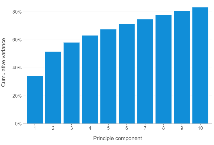
🗣️ CLASSROOM DISCUSSION: Do we notice anything in particular?
The amount of variance explained by each principle component decreases monotonically. If we look at the first 10 principle components, we can see that we have explained 83.5% of the data.
🎯 ACTION POINT: Use fit_transform on the cleaned data to create an array. Use pd.DataFrame() to transform this output into a singular data frame. Try using list comprehension to create a series of variable names such as pc1, …, pc19
# Employ fit_transform to create an array
pca_arrays = pipe.fit_transform(wvs_cleaned)

# Convert the array to a data frame and rename the columns
pca_df = pd.DataFrame(pca_arrays, columns=[f"pc{i+1}" for i in range(19)])
🎯 ACTION POINT: Plot the first two principle components.
(
    ggplot(pca_df, aes("pc1","pc2")) +
    geom_point(alpha = 0.05) +
    geom_smooth(method="lm")
)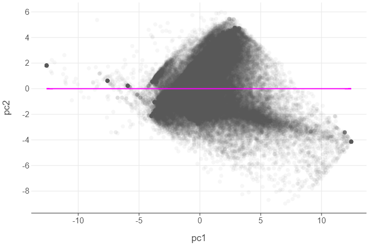
👨🏻🏫 TEACHING MOMENT: Why is there no correlation between the first and second principle components?
This is by design. PCA not only creates components which maximise the variance amongst the features, but also designs each component to be completely uncorrelated with one another!
We can further elaborate on each principle component by understanding the role each feature plays in influencing its loadings. We assess two aspects of the loadings:
Magnitude: larger absolute loadings show that a given feature will have a greater influence on the principle component.
Sign: positive / negative loadings indicate that a feature will contribute positively / negatively to the principle component.
# Create a list of data frames for each loading
list_dfs = [pd.DataFrame({"features":values,"loadings":comp}) for comp in pipe.named_steps["pca"].components_]

# Concatenate the list of data frames to create a singular data frame
loadings_df = pd.concat(list_dfs, keys = [i + 1 for i in range(19)], names = ["component","row"]).\
    reset_index().\
        drop(columns=["row"],index=1)

# Create a new column showing the absolute value of the loading
loadings_df["abs_loadings"] = np.abs(loadings_df["loadings"])
🎯 ACTION POINT: Plot the loadings of the first 4 principle components using a bar graph. Add facet_wrap(facets="component") to the plot to see the loading for each principle component in isolation.
(
    ggplot(loadings_df.query("component <= 4"), aes("loadings","features", fill = "abs_loadings")) +
    geom_bar(stat="identity") +
    facet_wrap(facets="component") +
    scale_fill_viridis() +
    theme(legend_position = "none")
)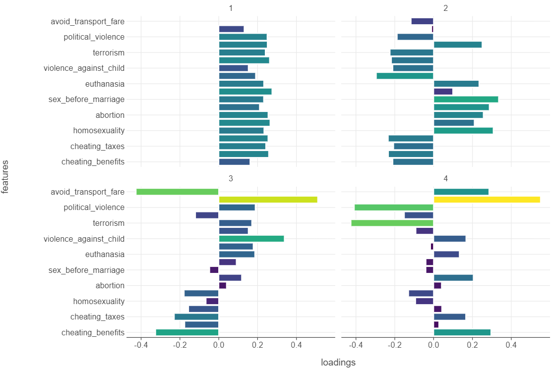
🗣️ CLASSROOM DISCUSSION: How can we describe each principle component?
- PC1: There are none that stand out - in fact, it looks like the principle component indicates moderate positions on all values / norms.
- PC2: Interestingly, we see that issues such as sex before marriage, abortion tend to positively influence the principle component and issues such as the use of violence tend to negatively influence the principle component.
- PC3: We see almost the flip side of PC2, although avoiding transport fairs and the death penalty influence the principle component the most.
- PC4: This is the most interesting. On the one hand, we see strong positive influence of the death penalty, yet political violence and terrorism strongly / negatively influence the principle component.
Part II: Using UMAP on the Varieties of Democracy Data Set (30 mins)
To round off our exploration of dimensionality reduction, we will look at UMAP (Uniform Manifold Approximation and Projection). UMAP, in essence, takes data that has a high number of dimensions and compresses it to a 2-dimensional feature space.
👉 NOTE: Andy Coenen and Adam Pearce of Google PAIR have put together an excellent tutorial on UMAP (click here).
vdem = pd.read_csv("../data/vdem-data-subset.csv")To explore this in the context of social science data, we will be looking at the Varieties of Democracy data set (2010-2023). Specifically, we will be looking at four different variables
v2x_polyarchy: Index of free and fair elections.v2x_libdem: Index of liberal democracy (protection of individuals / minorities from the tyranny of the state/majority).v2x_partip: Index of participatory democracy (participation of citizens in all political processes).regime: Four-fold typology of political regimes, namely, closed autocracy, electoral autocracy, electoral democracy, liberal democracy.
We will represent the three indices using a 3-d scatter plot, using colour to distinguish between regime type:
fig = px.scatter_3d(
    vdem,
    x="v2x_polyarchy",
    y="v2x_libdem",
    z="v2x_partipdem",
    color="regime",
    title="3D Scatter Plot of Democracy Variables"
)

fig.update_layout(
    scene=dict(
        xaxis_title="Polyarchy",
        yaxis_title="Liberal",
        zaxis_title="Participation"
    )
)

fig.show()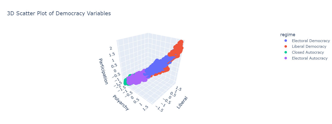
This is all good and well, but how can we represent this data as a 2-dimensional space? One increasingly popular method is UMAP. While we need to do some hand-waving as the mathematics are too complicated to be dealt with here, UMAP has a few key hyperparameters that can be experimented with.
- Number of nearest neighbours used to construct the initial high-dimensional graph (
n_neighbors). - Minimum distance between points in low dimensional space (
min_dist).
We will instantiate a UMAP, setting n_neighbors to 100, and fit it using our continuous features.
# Set a random seed
np.random.seed(123)
# Instantiate a UMAP with the relevant hyperparameter choice
reducer = UMAP(n_neighbors=100)
# Create a subset of the data using only variables beginning with "v2x"
vdem_subset = vdem[vdem.columns[vdem.columns.str.contains("v2x")]].to_numpy()
# Fit / transform the model to the subset of data to obtain the embeddings
embedding = reducer.fit_transform(vdem_subset)
# Convert the embeddings to a data frame
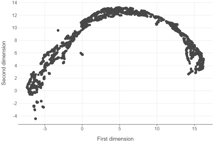
embedding = pd.DataFrame(embedding, columns = ["first_dim", "second_dim"])After this, we can extract the 2-d space created by UMAP and plot it.
(
    ggplot(embedding, aes("first_dim", "second_dim")) +
    geom_point() +
    labs(x = "First dimension", y = "Second dimension")
)
To see how this pertains to value labels, we can add the regime classifications to this plot.
# Add country/year and regime information to the embedding
embedding = pd.concat([embedding, vdem.filter(items=["country_year","regime"])], axis= 1)

# Plot the results
(
    ggplot(embedding, aes("first_dim", "second_dim", colour="regime")) +
    geom_point() +
    labs(x = "First dimension", y = "Second dimension", colour = "")
)
Note that UMAP has created a 2-map that maintains the topography of the data. Admittedly, this can be hard initially to interpret. However, we can note the following:
- This is a semi-circle configuration of points whereby less democratic regime types become more prominent.
- Despite this, we see considerable overlap between different regimes, indicating that considering these countries in at a given point in time to be distinctively democratic / autocratic may not be warranted in some cases.
- There is an outlier cluster that is distinct to the semi-circle configuration of points that UMAP provides. We can isolate these observations simply by filtering.
embedding.query("second_dim < -1.5")["country_year"].to_numpy()

array(['Burma/Myanmar-2022', 'Burma/Myanmar-2023', 'Yemen-2016',
       'Yemen-2017', 'Yemen-2018', 'Yemen-2019', 'Yemen-2020',
       'Yemen-2021', 'Yemen-2022', 'Yemen-2023', 'South Sudan-2017',
       'South Sudan-2018', 'South Sudan-2021', 'South Sudan-2022',
       'Afghanistan-2021', 'Afghanistan-2022', 'Afghanistan-2023',
       'North Korea-2010', 'North Korea-2011', 'North Korea-2012',
       'North Korea-2013', 'North Korea-2014', 'North Korea-2015',
       'North Korea-2016', 'North Korea-2017', 'North Korea-2018',
       'North Korea-2019', 'North Korea-2020', 'North Korea-2021',
       'North Korea-2022', 'North Korea-2023', 'Qatar-2010', 'Qatar-2011',
       'Qatar-2012', 'Qatar-2013', 'Qatar-2014', 'Qatar-2015',
       'Qatar-2016', 'Qatar-2017', 'Qatar-2018', 'Qatar-2019',
       'Qatar-2020', 'Qatar-2021', 'Qatar-2022', 'Qatar-2023',
       'Syria-2010', 'Syria-2011', 'Syria-2012', 'Syria-2013',
       'Syria-2014', 'Syria-2015', 'Syria-2016', 'Syria-2017',
       'Syria-2018', 'Syria-2019', 'Syria-2020', 'Syria-2021',
       'Syria-2022', 'Syria-2023', 'Belarus-2021', 'Belarus-2022',
       'Belarus-2023', 'China-2010', 'China-2011', 'China-2012',
       'China-2013', 'China-2014', 'China-2015', 'China-2016',
       'China-2017', 'China-2018', 'China-2019', 'China-2020',
       'China-2021', 'China-2022', 'China-2023', 'Eritrea-2010',
       'Eritrea-2011', 'Eritrea-2012', 'Eritrea-2013', 'Eritrea-2014',
       'Eritrea-2015', 'Eritrea-2016', 'Eritrea-2017', 'Eritrea-2018',
       'Eritrea-2019', 'Eritrea-2020', 'Eritrea-2021', 'Eritrea-2022',
       'Eritrea-2023', 'Libya-2010', 'Tajikistan-2016', 'Tajikistan-2017',
       'Tajikistan-2018', 'Tajikistan-2019', 'Tajikistan-2020',
       'Tajikistan-2021', 'Tajikistan-2022', 'Tajikistan-2023',
       'Turkmenistan-2010', 'Turkmenistan-2011', 'Turkmenistan-2012',
       'Turkmenistan-2013', 'Turkmenistan-2014', 'Turkmenistan-2015',
       'Turkmenistan-2016', 'Turkmenistan-2017', 'Turkmenistan-2018',
       'Turkmenistan-2019', 'Turkmenistan-2020', 'Turkmenistan-2021',
       'Turkmenistan-2022', 'Turkmenistan-2023', 'Uzbekistan-2010',
       'Uzbekistan-2011', 'Uzbekistan-2012', 'Uzbekistan-2013',
       'Uzbekistan-2014', 'Uzbekistan-2015', 'Uzbekistan-2016',
       'Bahrain-2011', 'Bahrain-2012', 'Bahrain-2013', 'Bahrain-2014',
       'Bahrain-2015', 'Bahrain-2016', 'Bahrain-2017', 'Bahrain-2018',
       'Bahrain-2019', 'Bahrain-2020', 'Bahrain-2021', 'Bahrain-2022',
       'Bahrain-2023', 'Equatorial Guinea-2010', 'Equatorial Guinea-2018',
       'Equatorial Guinea-2020', 'Equatorial Guinea-2021',
       'Equatorial Guinea-2022', 'Saudi Arabia-2010', 'Saudi Arabia-2011',
       'Saudi Arabia-2012', 'Saudi Arabia-2013', 'Saudi Arabia-2014',
       'Saudi Arabia-2015', 'Saudi Arabia-2016', 'Saudi Arabia-2017',
       'Saudi Arabia-2018', 'Saudi Arabia-2019', 'Saudi Arabia-2020',
       'Saudi Arabia-2021', 'Saudi Arabia-2022', 'Saudi Arabia-2023',
       'United Arab Emirates-2010', 'United Arab Emirates-2011',
       'United Arab Emirates-2012', 'United Arab Emirates-2013',
       'United Arab Emirates-2014', 'United Arab Emirates-2015',
       'United Arab Emirates-2016', 'United Arab Emirates-2017',
       'United Arab Emirates-2018', 'United Arab Emirates-2019',
       'United Arab Emirates-2020', 'United Arab Emirates-2021',
       'United Arab Emirates-2022', 'United Arab Emirates-2023'],
      dtype=object)
This approach yields a very interesting finding: the most notoriously undemocratic regimes in the world such as Afghanistan under the Taliban, North Korea, and Eritrea all form a part of this cluster.