💻 LSE DS202A 2024: Week 10 - Lab
This solution file follows the format of the Quarto file .qmd you had to fill in during the lab session. If you want to render the document yourselves and play with the code, you can download the .qmd version of this solution file by clicking on the button below:
🥅 Learning Objectives
- Perform basic feature engineering for text data using the
quantedaecosystem. - Apply feature engineering with text data to a supervised learning task.
- Compile structural topic models, using co-variates to predict topic prevalency.
⚙️ Setup
Install missing libraries:
There are a fair amount of new packages in this lab, but thankfully nearly all of them are on the CRAN. To install, you can rely upon the install.packages() function.
install.packages("bonsai")
install.packages("lightgbm")
install.packages("quanteda")
install.packages("quanteda.textstats")
install.packages("quanteda.textplots")
install.packages("quanteda.textmodels")
install.packages("shapviz")
install.packages("stm")
install.packages("devtools")
install.packages("vip")
To install the library tidystm, make sure you have devtools installed, then, in the console/R terminal, execute the following command
devtools::install_github("mikajoh/tidystm", dependencies = TRUE)Import required libraries:
library("bonsai")
library("ggsci")
library("lightgbm")
library("quanteda")
library("quanteda.textstats")
library("quanteda.textplots")
library("quanteda.textmodels")
library("shapviz")
library("stm")
library("tidyverse")
library("tidymodels")
library("tidystm")
# To install tidystm, copy + paste code into console.
# if (!require(devtools)) install.packages("devtools")
# devtools::install_github("mikajoh/tidystm", dependencies = TRUE)
library("vip")
A new data set: National Health Service (NHS) reviews (5 minutes)
nhs_reviews <-
  read_csv("data/NHS-reviews.csv") %>%
  as_tibble() %>%
  drop_na(review_positive)
Today, we will be looking at a data set of r ncol(nhs_reviews) reviews of the UK’s National Health Service.
review_title: The title of the review.review_text: The body of the review.star_rating: 1-5 rating of the NHS.review_positive: Whether the review was positive or negative.review_date: The date the review was left (YYYY-MM-DD).gp_response: Whether the general practitioner responded or not.
The column we are going to be taking a look at in more detail is review_text which contains a lot of information we can leverage. However, we first need to find a way of converting this raw text into usable features.
Enter quanteda (25 minutes)!
The most developed (and speedy) package for natural language processing in R is quanteda.
We will begin by transforming nhs_reviews into a corpus.
nhs_corpus <- corpus(nhs_reviews, text_field = "review_text")
nhs_corpus
Corpus consisting of 1,986 documents and 5 docvars.
text1 :
"Phoned up to book a appointment receptionist very helpful.Ad..."

text2 :
"Excellent efficient staffWell organised at dealing with a mi..."

text3 :
"I have always had an extremely good experience with my surge..."

text4 :
"Ive been told to wait in car and they will call me in an hou..."

text5 :
"Tried for over 2 hours to call the practice. When it was not..."

text6 :
"I have been with this surgery for more than 10 years and I a..."

[ reached max_ndoc ... 1,980 more documents ]
When we inspect the results, we can see that a corpus is simply a collection of documents with associated metadata. To access the metadata, we can run the following command.
nhs_corpus %>%
  docvars() %>%
  as_tibble()
# A tibble: 1,986 × 5
   review_title    star_rating review_positive review_date gp_response
   <chr>                 <dbl> <fct>           <date>      <chr>
 1 Great service             4 Positive        2021-10-13  Has not re…
 2 Friendly helpf…           5 Positive        2021-07-26  Responded
 3 Excellent serv…           5 Positive        2021-09-18  Has not re…
 4 Bizzare                   1 Negative        2021-06-19  Responded
 5 They want answ…           1 Negative        2021-06-12  Responded
 6 Creat practice            5 Positive        2021-08-23  Has not re…
 7 Very Helpful              5 Positive        2021-02-15  Responded
 8 GReat Practice            5 Positive        2021-01-15  Has not re…
 9 Great practice            5 Positive        2022-03-28  Has not re…
10 Needs an overh…           1 Negative        2022-05-07  Responded
# ℹ 1,976 more rows
# ℹ Use `print(n = ...)` to see more rows
👉 NOTE: This metadata will be utilised later on.
Next, we can convert each document in our corpus into a series of tokens.
🧑🏫 TEACHING MOMENT:
Tokens represent distinct words, punctuation, symbols, numbers etc. More advanced things we can do is create n-grams (combinations of two or more tokens) or use word stemming / lemmatisation. This, however, is beyond the scope of this course, so we will stick with unigrams.
nhs_tokens <-
  tokens(nhs_corpus,
         remove_punct = TRUE,
         remove_symbols = TRUE,
         remove_numbers = TRUE) %>%
  tokens_remove(pattern = stopwords("en"))

nhs_tokens
Tokens consisting of 1,986 documents and 5 docvars.
text1 :
 [1] "Phoned"          "book"            "appointment"
 [4] "receptionist"    "helpful.Advised" "Dr"
 [7] "ring"            "back"            "although"
[10] "little"          "late"            "understandable"
[ ... and 20 more ]

text2 :
 [1] "Excellent"    "efficient"    "staffWell"    "organised"
 [5] "dealing"      "minor"        "health"       "whilst"
 [9] "away"         "holiday"      "ordering"     "prescription"
[ ... and 4 more ]

text3 :
 [1] "always"        "extremely"     "good"          "experience"
 [5] "surgery"       "GP’s"          "Practice"      "Manager"
 [9] "Nurses"        "Receptionists" "helpful"       "professional"

text4 :
 [1] "Ive"      "told"     "wait"     "car"      "call"     "hour"
 [7] "called"   "didnt"    "even"     "see"      "daughter" "send"
[ ... and 17 more ]

text5 :
 [1] "Tried"    "hours"    "call"     "practice" "engaged"  "hold"
 [7] "least"    "minutes"  "hang"     "work"     "able"     "hang"
[ ... and 64 more ]

text6 :
 [1] "surgery"   "years"     "always"    "looked"    "doctors"
 [6] "try"       "best"      "referrals" "accepted"  "Reception"
[11] "staff"     "helpful"

[ reached max_ndoc ... 1,980 more documents ]
You will have noticed that we automatically filter out stopwords. This is because stopwords add little in the way of information about substantive topics and, as such, should not be considered.
👉 NOTE: We have used a pre-selected list of stopwords, however, you may need to employ a more nuanced list depending on your topic. For example, gender pronouns are included in the stopwords list which, in this case, could make sense but if you are studying topics relating to gender may not.
Next, we will convert this series of tokens into a document feature matrix (DFM).
nhs_dfm <-
  nhs_tokens %>%
  dfm() %>%
  dfm_trim(min_termfreq = 12)

nhs_dfm
Document-feature matrix of: 1,986 documents, 1,033 features (97.29% sparse) and 5 docvars.
       features
docs    phoned book appointment receptionist dr ring back although
  text1      1    1           1            2  2    1    1        1
  text2      0    0           0            0  0    0    0        0
  text3      0    0           0            0  0    0    0        0
  text4      0    0           0            0  0    0    0        0
  text5      0    0           2            0  0    0    1        0
  text6      0    0           0            0  0    0    0        0
       features
docs    little late
  text1      1    1
  text2      0    0
  text3      0    0
  text4      0    0
  text5      0    0
  text6      0    0
[ reached max_ndoc ... 1,980 more documents, reached max_nfeat ... 1,023 more features ]
👉 NOTE: quanteda is tidyverse friendly, so it is possible to achieve all these cleaning steps using one chunk of code, like so.
nhs_dfm <-
  nhs_reviews %>%
  corpus(text_field = "review_text") %>%
  tokens(remove_punct = TRUE, remove_symbols = TRUE, remove_numbers = TRUE) %>%
  tokens_remove(pattern = stopwords("en")) %>%
  dfm() %>%
  dfm_trim(min_termfreq = 12)
We set the minimum term frequency to 12, but any number around this threshold is probably appropriate. Not setting a threshold results in just over 7,500 features, many of which are not generalisable. A threshold of 12 results in a DFM with 1,033 features.
👉 NOTE: Try removing tokens_remove(pattern = stopwords("en")) and see what happens.
Now that we have our final DFM, we can use wordclouds to plot the relative frequency of each token.
textplot_wordcloud(nhs_dfm)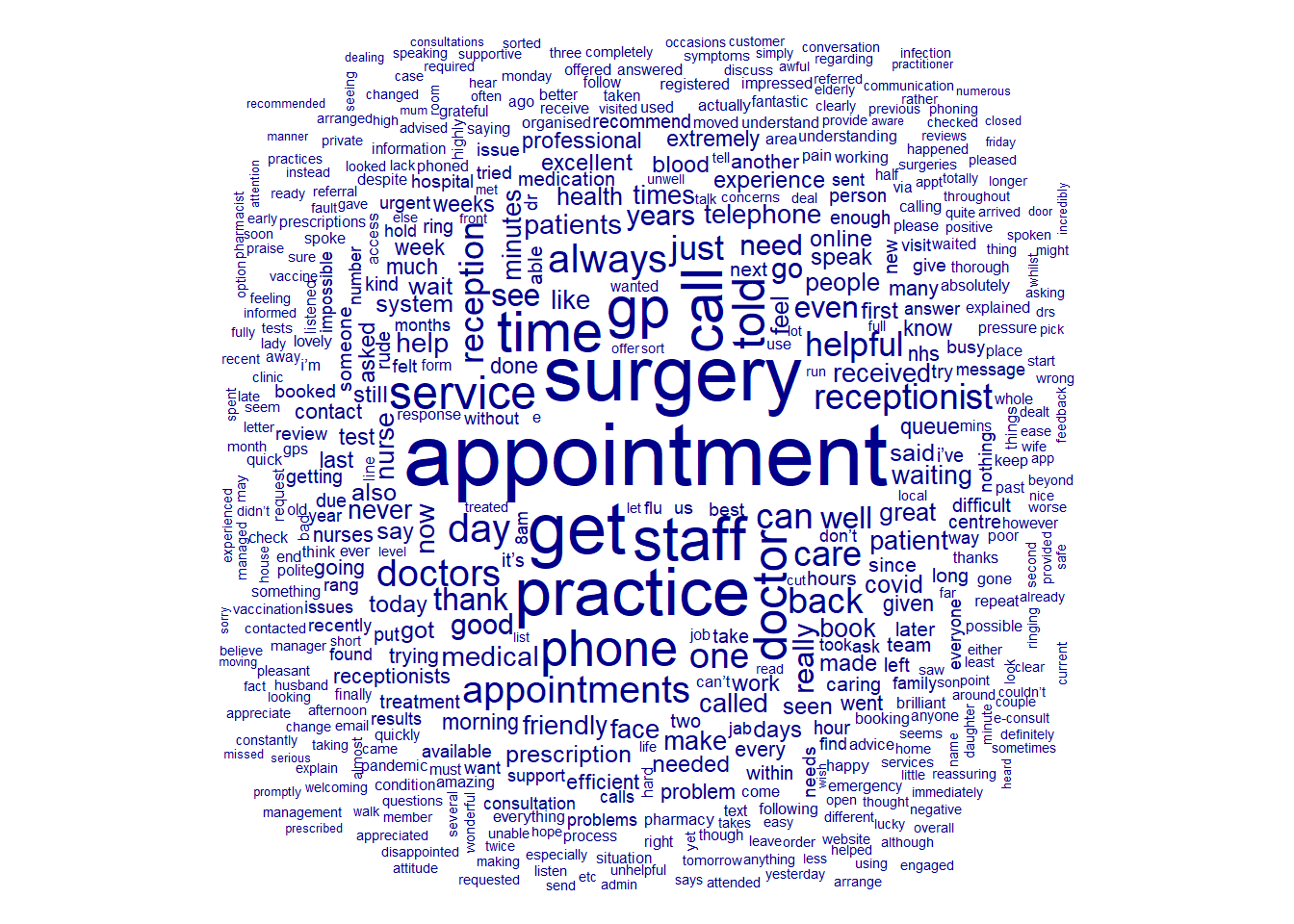
We can also plot the number of tokens in a given review, distinguishing between negative and positive reviews using colour.
tibble(ntoken = ntoken(nhs_tokens),
       positive = docvars(nhs_tokens)$review_positive) %>%
  ggplot(aes(ntoken, fill = positive)) +
  geom_density(alpha = 0.5) +
  theme_minimal() +
  theme(panel.grid.minor = element_blank(),
        panel.grid.major.x = element_blank(),
        legend.position = "bottom") +
  ggsci::scale_fill_lancet() +
  labs(x = "Number of tokens in document",
       y = "Density",
       fill = NULL)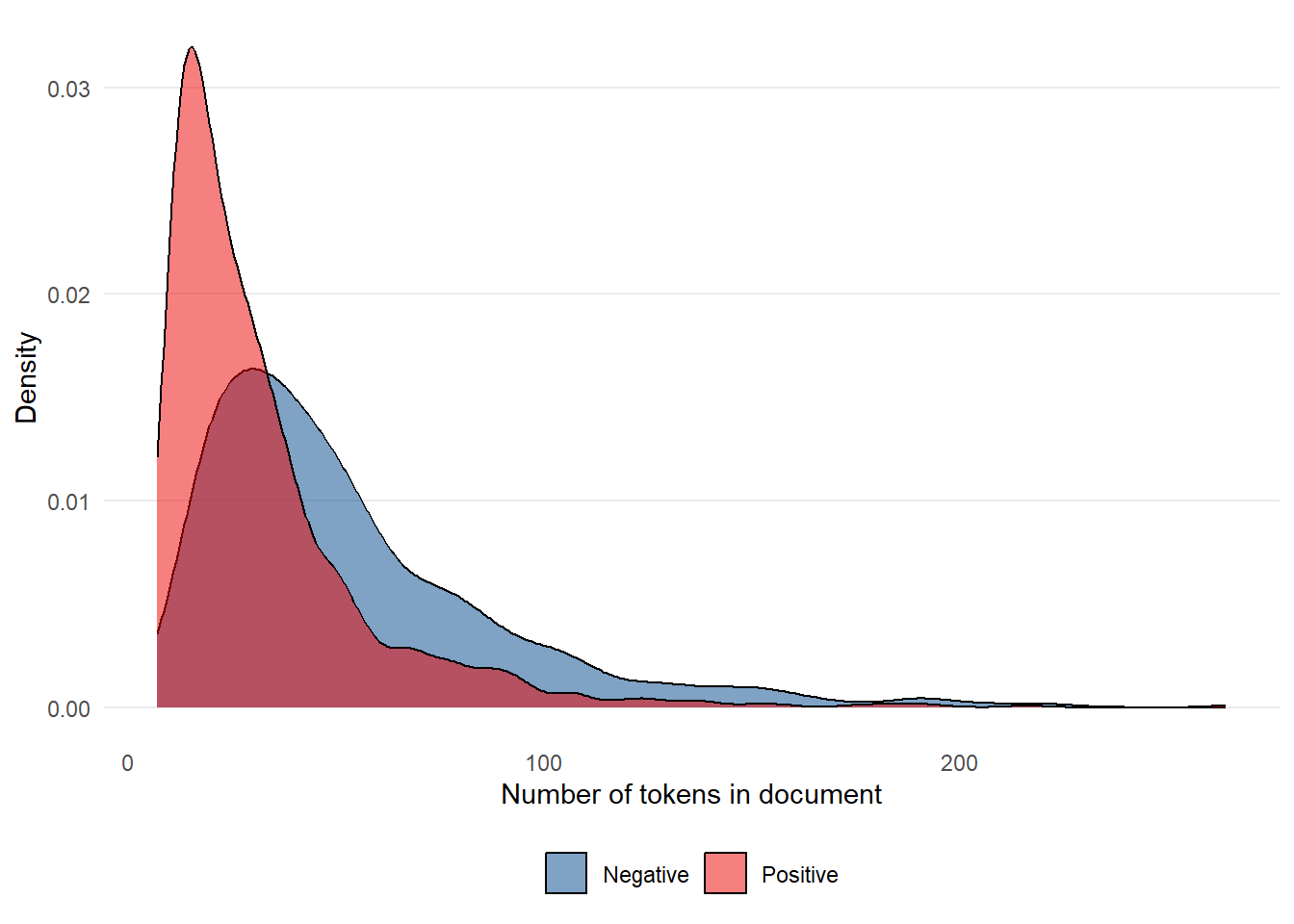
Supervised learning example: using tokens as features to identify positive reviews (30 minutes)
We can use our new feature engineering skills to predict whether or not an NHS review is positive. We can assess which terms are associated with positive and negative reviews using the keyness statistic.
positive_lgl <- docvars(nhs_dfm)$review_positive == "Positive"

tstat <- textstat_keyness(nhs_dfm, target = positive_lgl)

textplot_keyness(tstat) +
  labs(x = "Chi-Square Test")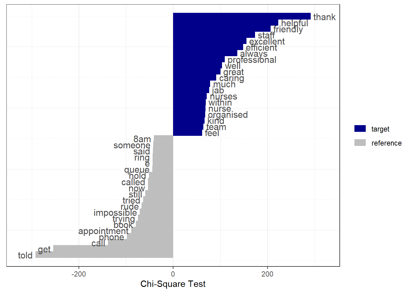
🗣️ CLASSROOM DISCUSSION:
Based on this graph, can we assess what issues tend to result in NHS users providing positive / negative reviews?
Helpful and caring staff seem to result in positive reviews. Queuing, rudeness, and phone calls seem to result in negative reviews.
To perform predictive modelling, we need to convert our DFM into a tibble, and add outcome labels found in the DFM metadata.
nhs_tbl <-
  nhs_dfm %>%
  convert(to = "data.frame") %>%
  mutate(positive = docvars(nhs_dfm)$review_positive,
         positive = as.factor(positive)) %>%
  as_tibble()
Next, we need to perform a training / testing split.
set.seed(321)

nhs_split <- initial_split(nhs_tbl, strata = positive)
nhs_train <- training(nhs_split)
nhs_test <- testing(nhs_split)
We then create a recipe. The only step we need to perform is to update the document ID variable to an ID so it is not used in the predictive model.
nhs_rec <-
  nhs_tbl %>%
  recipe(positive ~ .) %>%
  update_role(doc_id, new_role = "id")
After this, we will build a Light Gradient Boosted Model - similar to an XGBoost.
- Set
mtryto the square root of the number of features (minus 1), rounded to the nearest whole number. - Set
trees = 2000- we have a lot of features! - Set
learn_rate = 0.01. - Set the engine of the boosted tree to “lightgbm”, and include
importance = "impurity".
model <-
  boost_tree(mtry = round(sqrt(ncol(nhs_train) - 1),0), trees = 2000,
             learn_rate = 0.01) %>%
  set_mode("classification") %>%
  set_engine("lightgbm", importance = "impurity")
We can finally run the model. Use a workflow and add the recipe and model to it, then fit the workflow to the training data.
nhs_fit <-
  workflow() %>%
  add_recipe(nhs_rec) %>%
  add_model(model) %>%
  fit(data = nhs_train)
These steps should all be fairly straightforward. However, we are now going to find out which features are the most important, something we can do with tree-based models. We can do this using variable importance plots (VIPs) which, as the name suggests, visually ranks features in terms of their importance to the model as a whole.
nhs_fit %>%
  vip() +
  theme_minimal() +
  theme(panel.grid.minor = element_blank(),
        panel.grid.major.y = element_blank()) +
  labs(x = NULL, y = "Importance")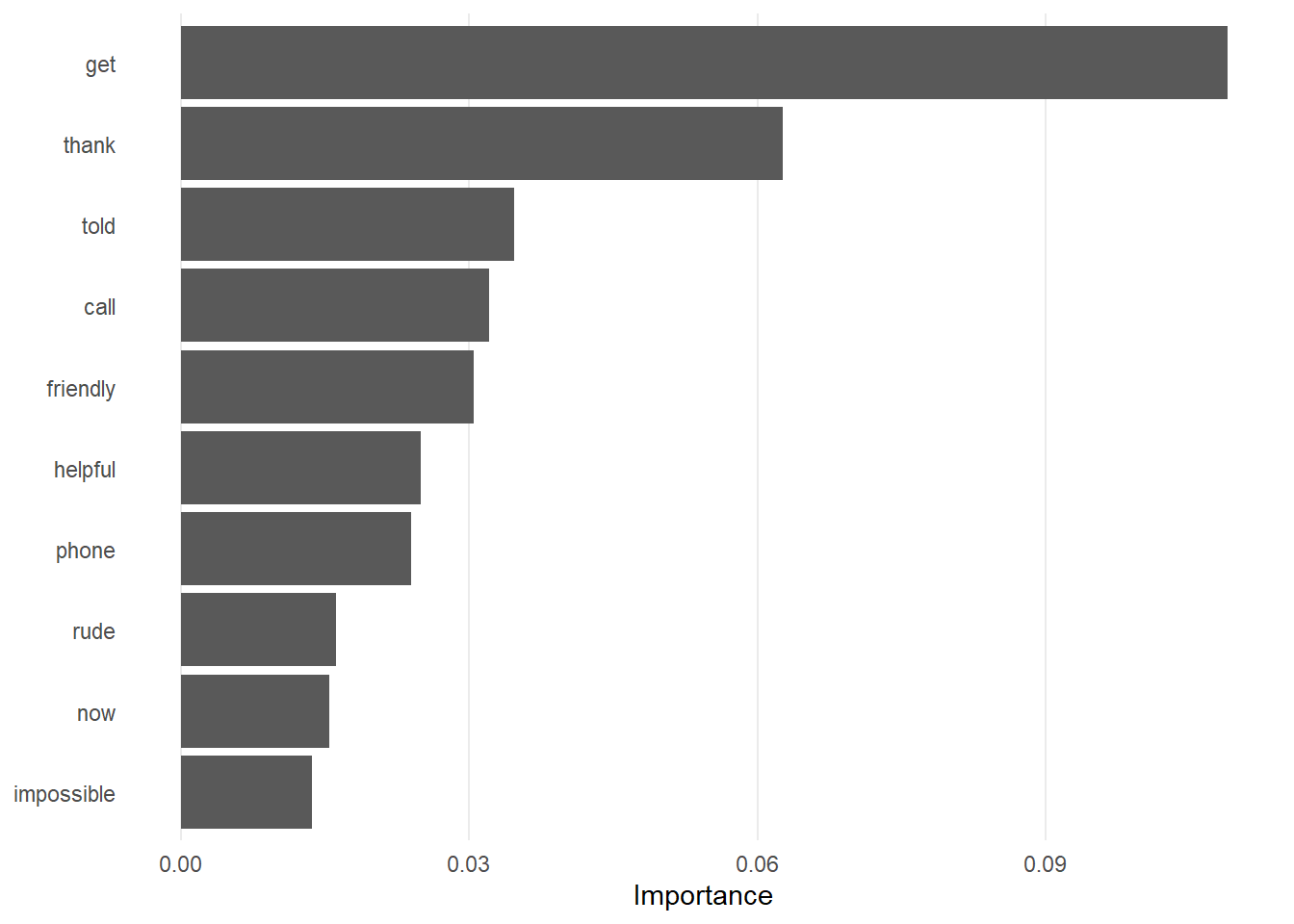
We can also use Shapley values, both for each observation and in the aggregate.
ℹ️ Information:
Shapley values have a game theoretical underpinning. The basic idea is that we want to assign “credit” to a given feature for improving the performance of a model when compared to all possible sets (or “coalitions”) of features. Instead of looking at the global contribution of each feature, as with variable importance, we compute the marginal contribution feature j makes to the prediction of an outcome for each observation, relative to the potential combination of features had the jth feature not been present. The Shapley value is then calculated as the average of all these marginal contributions across all observations. Shapley values can be calculated for all kinds of model, which makes them highly useful quantities of interest to calculate.
For a more in-depth look at Shapley values, check out “Interpretable Machine Learning” from Christoph Molnar (click here for the relevant section).
nhs_matrix <- as.matrix(select(nhs_train, -doc_id, -positive))
nhs_fit_extracted <- extract_fit_engine(nhs_fit)

shap <- shapviz(nhs_fit_extracted, X_pred = nhs_matrix, X = nhs_train)

sv_importance(shap, kind = "both", show_numbers = TRUE) +
  theme_minimal() +
  theme(panel.grid.minor = element_blank(),
        panel.grid.major.y = element_blank()) +
  labs(x = "SHAP value")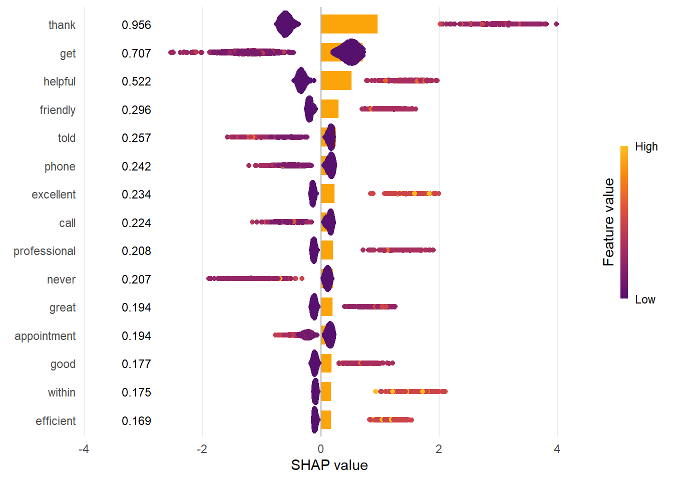
👉 NOTE:
If we enter ?sv_importance we will see that the bar plot shows the average absolute SHAP value per feature. The “beeswarm” plot displays SHAP values per row of data.
🗣️ CLASSROOM DISCUSSION:
Which features are most important? Which make the most sense?
“Thank”, “get”, “helpful”, “friendly”, and “phone” are the 5 most important features according to the Shapley values importance plot. Features such as “friendly” and “helpful” further indicate the reasons as to why people may review the NHS as positive.
Let’s apply this model to the test set. Present a confusion matrix.
nhs_fit %>%
  augment(new_data = nhs_test) %>%
  conf_mat(positive, .pred_class)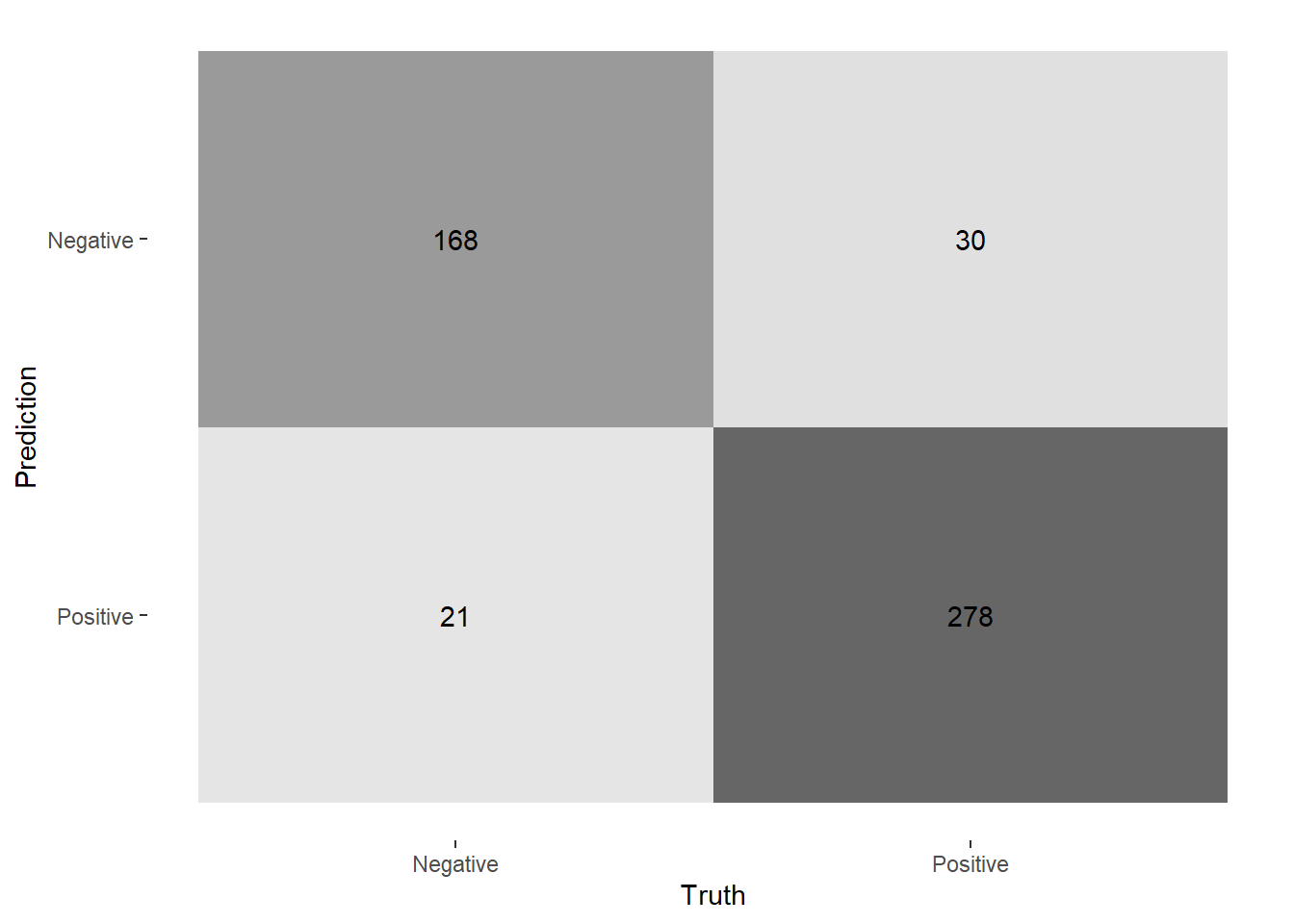
Use the f1-score to evaluate the model.
nhs_fit %>%
  augment(new_data = nhs_test) %>%
  f_meas(truth = positive, estimate = .pred_class)
# A tibble: 1 × 3
.metric .estimator .estimate
<chr> <chr> <dbl>
1 f_meas binary 0.868🗣️ CLASSROOM DISCUSSION:
How well does the model perform? Can you think of another model that could be a useful classifier?
The model has an f1-score of 0.87, which is quite good. Clearly, the bag-of-words approach has some merit when it comes to classifying NHS reviews. Another model that could add value is Lasso, as this can help us perform feature selection by shrinking insignificant features to zero - helpful when we have over 1,000 features!
Unsupervised learning example: using structural topic models (STMs) to understand important review themes (30 minutes)
Topic models are often used in social sciences to understand text data. These algorithms cluster words that are frequently used together across different documents into distinct topics (the number of which is set by the user). Each word is then ranked by how indicative they are of a given topic using some kind of score, of which there are many. We will use the FREX (frequency-exclusivity) score, as it finds words which are frequent in, and yet exclusive to, a given topic.
👉 NOTE:
More formally, FREX scores are the harmonic mean of rank of word by probability within a topic and rank by distribution of topic given the word.
Running a topic model is relatively straightforward. We will pick 10 topics - check out the bonus section to find out why. All we need to do is feed stm our DFM and specify K.
nhs_tm <- stm(nhs_dfm, K = 10)👉 NOTE: This may take a few minutes to compile. Please be patient!
After the model compiles, we can review the top 7 terms associated with each topic, based on FREX scores.
labelTopics(nhs_tm)$frex %>% t() [,1] [,2] [,3] [,4]
[1,] "consultation" "since" "always" "get"
[2,] "dr" "repeat" "nurses" "book"
[3,] "face" "website" "best" "available"
[4,] "tests" "registered" "highly" "appointments"
[5,] "treatment" "ago" "great" "impossible"
[6,] "contacted" "app" "care" "system"
[7,] "given" "prescriptions" "staff" "try"
[,5] [,6] [,7] [,8] [,9]
[1,] "test" "jab" "i’ve" "told" "process"
[2,] "blood" "flu" "team" "message" "vaccine"
[3,] "appt" "clinic" "drs" "hold" "ease"
[4,] "rude" "organised" "past" "call" "well"
[5,] "negative" "efficient" "family" "said" "felt"
[6,] "sample" "covid" "spoken" "waited" "safe"
[7,] "read" "vaccination" "practise" "called" "done"
[,10]
[1,] "advice"
[2,] "lovely"
[3,] "nice"
[4,] "saw"
[5,] "fantastic"
[6,] "nurse"
[7,] "really" 🗣️ CLASSROOM DISCUSSION:
Can you figure out the “topic” using these words?
Topic 1
Consultation with a relevant doctor and / or delivery of treatment / test results.
Topic 2
Access to prescriptions and using the NHS website.
Topic 3
Nursing staff.
Topic 4
Booking appointments.
Topic 5
Blood tests.
Topic 6
COVID-19 vaccine appointments.
Topic 7
Family practices.
Topic 8
Phone call waiting times.
Topic 9
Other vaccine appointments.
Topic 10
Advice given by nurses.
Already, we can see that topic models certainly provide intuitive insight into these NHS reviews. However, suppose that we now think that a given topic may be more prominent in positive / negative reviews? We can add covariates such as review_positive to our topic model to statistically test this hypothesis.
positive <- docvars(nhs_dfm)$review_positive
nhs_tm_prev <- stm(nhs_dfm, K = 10, prevalence = ~ positive)
After compiling the model. We can then run the following command which estimates the probability that a topic occurs based on whether or not a review is positive.
effects <- estimateEffect(1:10 ~ positive, nhs_tm_prev)
summary(effects)
Call:
estimateEffect(formula = 1:10 ~ positive, stmobj = nhs_tm_prev)


Topic 1:

Coefficients:
                 Estimate Std. Error t value Pr(>|t|)
(Intercept)      0.060495   0.006242   9.692  < 2e-16 ***
positivePositive 0.067465   0.008423   8.010 1.94e-15 ***
---
Signif. codes:  0 ‘***’ 0.001 ‘**’ 0.01 ‘*’ 0.05 ‘.’ 0.1 ‘ ’ 1


Topic 2:

Coefficients:
                  Estimate Std. Error t value Pr(>|t|)
(Intercept)       0.139226   0.006368  21.864   <2e-16 ***
positivePositive -0.073415   0.008021  -9.152   <2e-16 ***
---
Signif. codes:  0 ‘***’ 0.001 ‘**’ 0.01 ‘*’ 0.05 ‘.’ 0.1 ‘ ’ 1


Topic 3:

Coefficients:
                 Estimate Std. Error t value Pr(>|t|)
(Intercept)      0.030336   0.007300   4.156 3.38e-05 ***
positivePositive 0.203678   0.009993  20.382  < 2e-16 ***
---
Signif. codes:  0 ‘***’ 0.001 ‘**’ 0.01 ‘*’ 0.05 ‘.’ 0.1 ‘ ’ 1


Topic 4:

Coefficients:
                  Estimate Std. Error t value Pr(>|t|)
(Intercept)       0.259940   0.008585   30.28   <2e-16 ***
positivePositive -0.202644   0.009984  -20.30   <2e-16 ***
---
Signif. codes:  0 ‘***’ 0.001 ‘**’ 0.01 ‘*’ 0.05 ‘.’ 0.1 ‘ ’ 1


Topic 5:

Coefficients:
                  Estimate Std. Error t value Pr(>|t|)
(Intercept)       0.115554   0.006259  18.463  < 2e-16 ***
positivePositive -0.054419   0.007348  -7.406 1.92e-13 ***
---
Signif. codes:  0 ‘***’ 0.001 ‘**’ 0.01 ‘*’ 0.05 ‘.’ 0.1 ‘ ’ 1


Topic 6:

Coefficients:
                 Estimate Std. Error t value Pr(>|t|)
(Intercept)      0.021392   0.006182    3.46 0.000551 ***
positivePositive 0.107273   0.008560   12.53  < 2e-16 ***
---
Signif. codes:  0 ‘***’ 0.001 ‘**’ 0.01 ‘*’ 0.05 ‘.’ 0.1 ‘ ’ 1


Topic 7:

Coefficients:
                 Estimate Std. Error t value Pr(>|t|)
(Intercept)      0.059058   0.005333  11.074   <2e-16 ***
positivePositive 0.015073   0.006960   2.166   0.0305 *
---
Signif. codes:  0 ‘***’ 0.001 ‘**’ 0.01 ‘*’ 0.05 ‘.’ 0.1 ‘ ’ 1


Topic 8:

Coefficients:
                 Estimate Std. Error t value Pr(>|t|)
(Intercept)       0.27014    0.00835   32.35   <2e-16 ***
positivePositive -0.22139    0.01013  -21.85   <2e-16 ***
---
Signif. codes:  0 ‘***’ 0.001 ‘**’ 0.01 ‘*’ 0.05 ‘.’ 0.1 ‘ ’ 1


Topic 9:

Coefficients:
                 Estimate Std. Error t value Pr(>|t|)
(Intercept)      0.025716   0.004850   5.302 1.27e-07 ***
positivePositive 0.067464   0.007278   9.269  < 2e-16 ***
---
Signif. codes:  0 ‘***’ 0.001 ‘**’ 0.01 ‘*’ 0.05 ‘.’ 0.1 ‘ ’ 1


Topic 10:

Coefficients:
                 Estimate Std. Error t value Pr(>|t|)
(Intercept)      0.018056   0.004550   3.969 7.49e-05 ***
positivePositive 0.091132   0.006761  13.478  < 2e-16 ***
---
Signif. codes:  0 ‘***’ 0.001 ‘**’ 0.01 ‘*’ 0.05 ‘.’ 0.1 ‘ ’ 1
This is all well and good, but it is hard to determine which topic relates to which coefficient. The below graph makes things a bit easier for the user to understand.
labels <-
  labelTopics(nhs_tm_prev)$frex %>%
  as_tibble() %>%
  unite(everything(), col = "words", sep = ", ")

extract.estimateEffect(effects, "positive", model = nhs_tm_prev, method = "difference", cov.value1 = "Positive", cov.value2 = "Negative") %>%
  as_tibble() %>%
  bind_cols(labels) %>%
  mutate(words = fct_inorder(as.factor(words))) %>%
  ggplot(aes(estimate, as.character(topic))) +
  facet_wrap(. ~ words, ncol = 1, scales = "free_y") +
  geom_vline(xintercept = 0) +
  geom_point(position = position_dodge(width = 1)) +
  geom_linerange(aes(xmin = ci.lower, xmax = ci.upper),
                 position = position_dodge(width = 1)) +
  theme_minimal() +
  theme(panel.grid.minor = element_blank(),
        panel.grid.major.y = element_blank(),
        axis.title.y = element_text(angle = 0)) +
  labs(x = "Coefficient estimate\n(95% confidence interval)",
       y = "Topic\nnumber",
       title = "What topics are most prevalent in positive NHS reviews?",
       subtitle = "Coefficient estimates of a structural topic model (K=5) with topic prevalency predicted by positive reviews",
       caption = "Note: Top 7 words for each topic determined by FREX score.")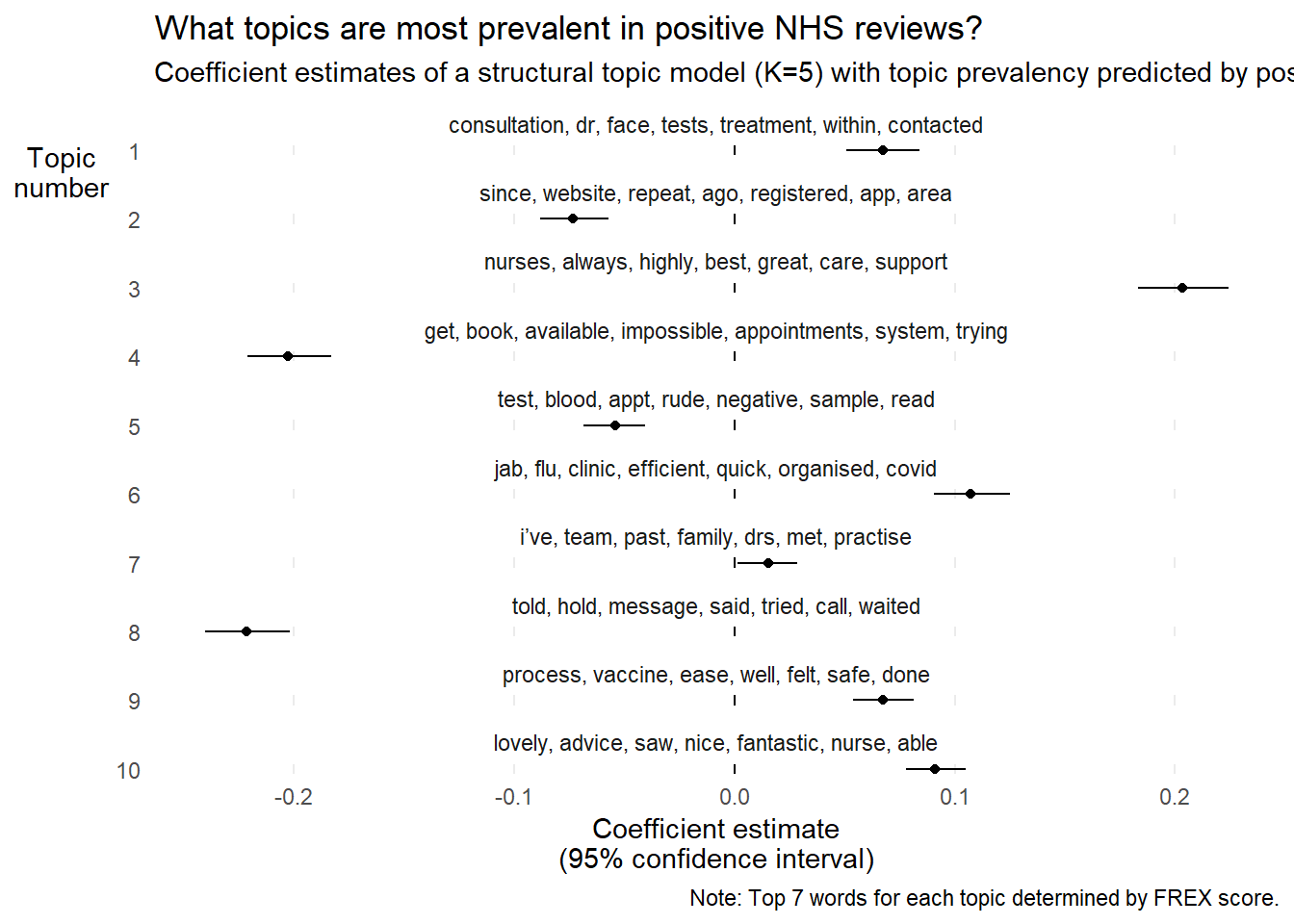
🗣️ CLASSROOM DISCUSSION:
Do these coefficient estimates make sense?
Yes, they more or less correspond to our intuitions. Issues relating to waiting times and accessing repeat prescriptions are more prevalent in negative reviews. Consultations with doctors, and friendly / efficient staff are more prevalent in positive reviews.
Bonus: What is the optimal number of topics?
Much like finding the optimal number of clusters with k-means, finding the optimal number of topics is by no means straightforward. We adapt a process similar to that presented in Weston et al (2023).
We will try different values of K (3 to 20) and assess the following statistics. Quoting Weston et al (2023: 4):
“Exclusivity represents the degree to which words are exclusive to a single topic rather than associated with multiple topics. Exclusive words are more likely to carry topic-relevant content, thus assisting with the interpretation of topics … Variational lower bound is the metric used to determine convergence for a specific solution. In other words, the estimation functions … will continue to evaluate models until the change in the variational lower bound is smaller than some designated threshold or the maximum number of allowed iterations is reached. The default value for convergence is change less than .00001. Residual is the estimation of the dispersion of residuals for a particular solution … Some have recommended looking for local minima … whereas others suggest that dispersion greater than one indicates more topics are needed. Finally, semantic coherence is a measure of how commonly the most probable words in a topic co-occur … A limitation of semantic coherence is that it is highest when the number of topics is low.”
doParallel::registerDoParallel()

k_search <- searchK(
  nhs_dfm,
  K = c(3:20),
  N = 500,
  heldout.seed = 123
)

k_search$results %>%
  pivot_longer(-K, names_to = "metric", values_to = "value") %>%
  filter(metric %in% c("exclus", "semcoh", "lbound", "residual")) %>%
  unnest(c(K, value)) %>%
  mutate(metric = case_when(metric == "exclus" ~ "Exclusivity",
                            metric == "lbound" ~ "Lower Bound",
                            metric == "residual" ~ "Residual Dispersion",
                            .default = "Semantic Coherence")) %>%
  ggplot(aes(K, value, colour = metric)) +
  facet_wrap(. ~ metric, scales = "free_y") +
  geom_vline(xintercept = c(5, 10), linetype = "dashed") +
  geom_point() +
  geom_line() +
  theme_minimal() +
  theme(panel.grid.minor = element_blank(),
        panel.grid.major.x = element_blank(),
        strip.text = element_text(size = 15, hjust = 0),
        legend.position = "none") +
  scale_colour_uchicago() +
  labs(y = NULL)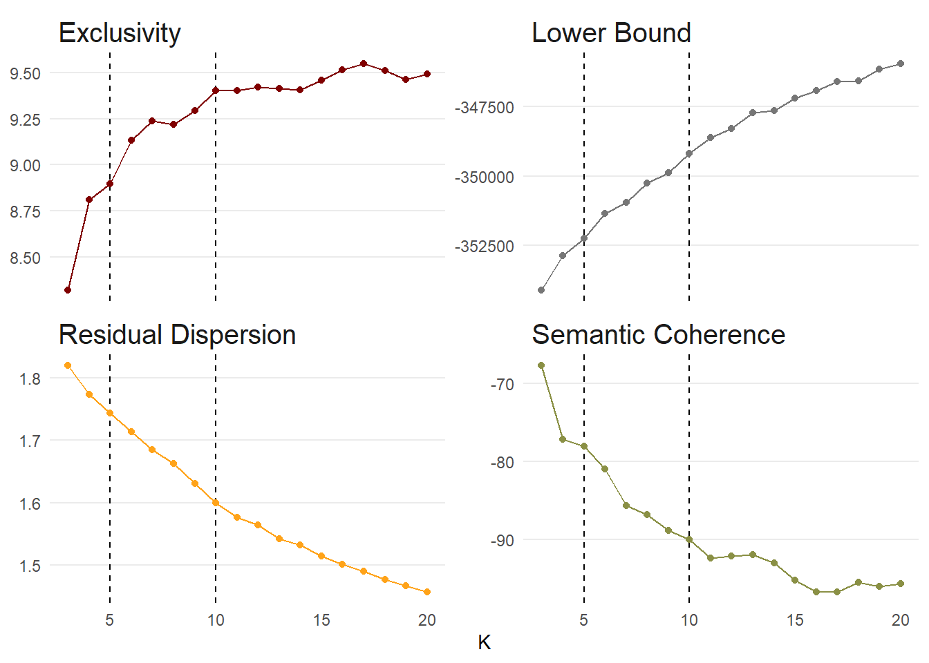
👉 NOTE: This will take a few minutes to compile. Please be patient!
❓ Question:
Based on these graphs, which K is best?
It is hard to provide a truly conclusive answer in this case. Beyond 10 topics, we only gain small increases in exclusivity. Between 4 and 5 topics would be better for semantic coherence, but recall that semantic coherence is automatically higher for topic models with a lower number of topics. We further see a continued drop off in semantic coherence after 10 topics which indicate that a topic number larger than this would be less coherent. Residual dispersion / variational lower bound decreases / increases consistently as the number of topics increase, indicating that a higher number of topics within the range would be better than a lower number. As a result, we could make the case that 10 topics is most suitable in this instance.
