
💻 LSE DS202W 2023: Week 11 - Lab
2023/24 Winter Term
In our final lab of DS202W, you will learn how to use quanteda, an R package for quantitative text analysis. We will do more data pre-processing, and you will have the chance to apply dimensionality reduction (e.g., PCA) and clustering (e.g., k-means) techniques to text data.
🥅 Learning Objectives
- Pre-processing: Learn how to use the
quantedapackage to pre-process text data - Text summarisation: Learn how to use the
quantedapackage to summarise text data - Reinforce dimensionality reduction and clustering: Apply dimensionality reduction and clustering techniques to text data
- Discover a new way to find out the optimal number of clusters: Learn how to use the
NbClustpackage to determine the optimal number of clusters - Visualisation: Learn how to use the
plotlypackage to visualise text data
However, the most critical aspect of this lab is that you will not be asked to produce code. Instead, you will be asked to interpret the results of the code we provide you with. Discussing the results with your peers will be key to your success in this lab.
This will help you practice for your Summative 03 and Summer exams. Those assignments will not require you to write code unless you want to get extra credit.
📚 Preparation
Use the link below to download the lab file:
Install new packages
In the R Console – never in the Quarto Markdown – run the following commands:
install.packages("ggsci")
install.packages("plotly")
install.packages("NbClust")
install.packages("janitor")
install.packages("topicmodels")


## Quanteda packages
install.packages("quanteda")
install.packages("quanteda.textstats")
install.packages("quanteda.textplots")
install.packages("quanteda.textmodels")
Note: if quanteda installs fine, but you get the weird and mysterious error below, your R setup is likely conflicting with your renv setup.
Error: package or namespace load failed for ‘quanteda’:
 .onLoad failed in loadNamespace() for 'RcppParallel', details:
  call: dyn.load(file, DLLpath = DLLpath, ...)
  error: unable to load shared object ...
Without getting into too many details here, you can just deactivate renv for now:
renv::deactivate()Then, try to load all the libraries again.
Packages you will need
library(tidyverse)
library(tidymodels)

library(janitor)     # for better names and other data cleaning tools
library(plotly)      # for interactive charts

library(NbClust)     # to calculate the optimal number of clusters
library(topicmodels) # for topic modeling

library(quanteda)
library(quanteda.textstats)
library(quanteda.textplots)
library(quanteda.textmodels)

# Vanity packages:
library(ggsci)       # we like pretty colours
📋 Lab Tasks
No need to wait! Start tackling the action points below when you come to the classroom.
Part 0: Export your chat logs (~ 3 min)
As part of the  GENIAL project, we ask that you fill out the following form as soon as you come to the lab:
🎯 ACTION POINTS
🔗 CLICK HERE to export your chat log.
Thanks for being GENIAL! You are now one step closer to earning some prizes! 🎟️
👉 NOTE: You MUST complete the initial form.
If you really don’t want to participate in GENIAL1, just answer ‘No’ to the Terms & Conditions question - your e-mail address will be deleted from GENIAL’s database the following week.
Part I - Meet a new dataset (15 mins)
This dataset we are going to use today, Political Apologies across Cultures (PAC), was assembled by the Political Apologies x Cultures project. The data consists of an inventory of political apologies offered by states or state representatives to a collective for human rights violations that happened in the recent or distant past.
🎯 ACTION POINTS
Go to the Political Apologies x Cultures project website, click on Database and then click on Coded Database. This will download a file called
PAC_Coded-Apologies_Public-Version-2.xlsxto your computer.Before opening it in R, take some time to look at the data in its raw format using MS Excel (or Google Sheets). What do you see? Which tabs and columns seem interesting?
Create a
df_pacand pre-process thedate_originalcolumn. We can use theread_excelfunction from the tidyverse packagereadxlto read Excel spreadsheets:
df_pac <-
  readxl::read_excel("PAC_Coded-Apologies_Public-Version-2.xlsx",
                     sheet="PAC_coding_Template",
                     .name_repair="minimal") %>%
  janitor::clean_names() %>%
  drop_na(date_original) %>%
  mutate(date_original=
          case_when(
            str_starts(date_original, "0.0.") ~ str_replace(date_original, "0.0.", "1.1."), str_starts(date_original, "0.")   ~ str_replace(date_original, "0.", "1."),
            .default=date_original),
         date_original=lubridate::dmy(date_original))  %>%
  arrange(desc(date_original))

df_pac %>% glimpse()
Click here to see the output
Rows: 396
Columns: 91
$ no                         <dbl> 512, 511, 509, 498, 497, 493, 487, 506, 503, 490, 489, 507, 500, 486, 482,…
$ date_original              <date> 2022-07-11, 2022-06-08, 2022-03-23, 2022-03-10, 2022-02-17, 2021-12-13, 2…
$ date                       <chr> "11.07.2022", "08.06.2022", "23.03.2022", "10.03.2022", "17.02.2022", "13.…
$ year_1                     <dbl> 2022, 2022, 2022, 2022, 2022, 2021, 2021, 2021, 2021, 2021, 2021, 2021, 20…
$ year_2                     <dbl> 10, 10, 10, 10, 10, 10, 10, 10, 10, 10, 10, 10, 10, 10, 10, 10, 10, 10, 10…
$ year_cat                   <chr> "10 =2020-2024", "10 =2020-2024", "10 =2020-2024", "10 =2020-2024", "10 =2…
$ description                <chr> "Dutch Minister of Defence Kasja Ollongren offered 'deepest apologies' for…
$ country_s                  <chr> "Netherlands", "Belgium", "United Kingdom of Great Britain and Northern Ir…
$ check_country_s            <chr> "Netherlands", "Belgium", "United Kingdom of Great Britain and Northern Ir…
$ count_s_iso_alpha          <chr> "NLD", "BEL", "GBR", "DNK", "NLD", "CAN", "NLD", "SVK", "ISR", "MEX", "FRA…
$ count_s_iso_num            <dbl> 528, 56, 826, 208, 528, 124, 528, 703, 376, 484, 250, 703, 68, 554, 276, 2…
$ region_s_un                <dbl> 150, 150, 150, 150, 150, 19, 150, 150, 142, 19, 150, 150, 19, 9, 150, 150,…
$ region_s_oecd              <chr> "Europe", "Europe", "Europe", "Europe", "Europe", "Americas", "Europe", "E…
$ name_send                  <chr> "Kasja Ollongren", "Philippe of Belgium", "Prince William", "Mette Frederi…
$ role_send                  <chr> "4 =Minister", "1 =King/Queen/Emperor", "8 =Other official role", "3 =Prim…
$ role_send_specify_other    <chr> NA, NA, "Prince", NA, NA, NA, NA, NA, NA, NA, NA, NA, NA, NA, NA, NA, NA, …
$ off_send                   <chr> "0 =No", "0 =No", "0 =No", "0 =No", "0 =No", "1 =No", "0 =No", "0 =No", "0…
$ political_party            <chr> "Democrats 66", NA, NA, "Social Democratic Party", "VVD (People's Party fo…
$ political_color            <chr> "5 =Centre-left", NA, NA, "5 =Centre-left", "9 =Centre-right", "6 =Centre …
$ count_rec                  <chr> "Bosnia and Herzegovina", "Democratic Republic of the Congo", "Jamaica", "…
$ check_count_rec            <chr> "Bosnia and Herzegovina", "Democratic Republic of the Congo", "Jamaica", "…
$ count_r_iso_alpha          <chr> "BIH", "COD", "JAM", "GRL", "IDN", "CAN", "NLD", "SVK", "ISR", "MEX", "FRA…
$ count_r_iso_num            <chr> "70", "180", "388", "304", "360", "124", "528", "703", "376", "484", "250"…
$ region_r_un                <chr> "150", "2", "19", "19", "142", "19", "150", "150", "142", "19", "150", "*T…
$ region_r_oecd              <chr> "Europe", "Africa", "Americas", "Americas", "Asia", "Americas", "Europe", …
$ group_rec_id_1             <chr> "3 =Ethnicity/race", "1 =Nation/citizenship", "3 =Ethnicity/race", "6 =Tri…
$ group_rec_id_2             <chr> NA, NA, NA, NA, NA, NA, NA, NA, NA, NA, NA, "5 =Religion/spiritual faith",…
$ group_rec_id_3             <chr> NA, NA, NA, NA, NA, NA, NA, NA, NA, NA, NA, NA, NA, NA, NA, NA, NA, NA, NA…
$ group_rec_id_specify_other <chr> NA, NA, NA, NA, NA, NA, NA, NA, NA, NA, NA, NA, "Civilians during post-ele…
$ group_rec_1                <chr> "2 =Between-country", "2 =Between-country", "2 =Between-country", "2 =Betw…
$ group_rec_1_1              <chr> NA, NA, NA, NA, NA, NA, "1 =Minority", NA, NA, NA, NA, NA, NA, "1 =Minorit…
$ group_rec_2                <chr> "3 =Both primary and secondary victim-groups", "3 =Both primary and second…
$ context_1                  <chr> "War: Yugoslav wars", "Colonial rule: Belgium - Congo", "Slavery", "Maltre…
$ context_2                  <chr> NA, NA, NA, NA, "War: Netherlands - Indonesia", NA, NA, NA, NA, NA, NA, NA…
$ context_3                  <chr> NA, NA, NA, NA, NA, NA, NA, NA, NA, NA, NA, NA, NA, NA, NA, NA, NA, NA, NA…
$ context_cat_1              <chr> "War", "Colonial rule", "Slavery", "Treatment of indigenous population", "…
$ context_cat_2              <chr> NA, NA, NA, NA, "War", NA, NA, NA, "Settler colonialism", NA, NA, NA, NA, …
$ context_cat_3              <lgl> NA, NA, NA, NA, NA, NA, NA, NA, NA, NA, NA, NA, NA, NA, NA, NA, NA, NA, NA…
$ hrv_1                      <chr> "20 =Not specified", "6 =Colonization", "4 =Forced labor/slavery", "17 =Fo…
$ hrv_2                      <chr> NA, "8 =Racism/discrimination", NA, NA, NA, NA, NA, NA, NA, "3 =Murder/exe…
$ hrv_3                      <chr> NA, NA, NA, NA, NA, NA, NA, NA, NA, "4 =Forced labor/slavery", NA, NA, NA,…
$ hrv_specify_other          <chr> NA, NA, NA, NA, NA, NA, NA, NA, NA, NA, NA, NA, NA, NA, NA, NA, NA, NA, NA…
$ hrv_date_start             <dbl> 1995, 1885, 1562, 1951, 1945, NA, 1985, 1966, 1956, 1876, 1962, 1939, 2019…
$ hrv_date_end               <dbl> 1995, 1960, 1807, NA, 1949, NA, 2014, 2004, 1956, 1910, NA, 1945, 2019, 19…
$ time_hrv_start             <dbl> 27, 137, 460, 71, 77, NA, 36, 55, 65, 145, 59, 82, 2, 48, 117, 27, 81, 44,…
$ time_hrv_end               <dbl> 27, 62, 215, NA, 73, NA, 7, 17, 65, 111, NA, 76, 2, 42, 113, 27, 76, 44, 5…
$ apol_set                   <chr> "5 =Commemoration", "7 =(Diplomatic) visit", "7 =(Diplomatic) visit", "1 =…
$ apol_set_specify_other     <chr> NA, NA, NA, "Ceremony with victims", NA, "Via a public livestream on Faceb…
$ apol_med                   <chr> "1 =Verbal", "1 =Verbal", "1 =Verbal", "1 =Verbal", "1 =Verbal", "1 =Verba…
$ apol_lang                  <chr> "nld =Dutch", "fra =French", "eng =English", "dan =Danish", "nld =Dutch", …
$ apol_lang_2                <chr> NA, NA, NA, NA, NA, NA, NA, NA, "ara =Arabic", NA, NA, NA, NA, NA, NA, NA,…
$ apol_text                  <chr> "2 =Full text", "2 =Full text", "2 =Full text", "2 =Full text", "2 =Full t…
$ apol_trans                 <chr> "0 =No translation", "4 =Translation found elsewhere", "1 =Original Englis…
$ apol_light                 <chr> "0 = Completer apology", "0 = Completer apology", "0 = Completer apology",…
$ gini                       <chr> NA, NA, NA, NA, NA, NA, NA, NA, NA, NA, NA, NA, NA, NA, NA, NA, NA, NA, NA…
$ wvs_y003                   <chr> NA, NA, NA, NA, NA, NA, NA, NA, NA, NA, NA, NA, NA, NA, NA, NA, NA, NA, NA…
$ wvs_a189                   <chr> NA, NA, NA, NA, NA, NA, NA, NA, NA, NA, NA, NA, NA, NA, NA, NA, NA, NA, NA…
$ wvs_a190                   <chr> NA, NA, NA, NA, NA, NA, NA, NA, NA, NA, NA, NA, NA, NA, NA, NA, NA, NA, NA…
$ wvs_a191                   <chr> NA, NA, NA, NA, NA, NA, NA, NA, NA, NA, NA, NA, NA, NA, NA, NA, NA, NA, NA…
$ wvs_a192                   <chr> NA, NA, NA, NA, NA, NA, NA, NA, NA, NA, NA, NA, NA, NA, NA, NA, NA, NA, NA…
$ wvs_a193                   <chr> NA, NA, NA, NA, NA, NA, NA, NA, NA, NA, NA, NA, NA, NA, NA, NA, NA, NA, NA…
$ wvs_a194                   <chr> NA, NA, NA, NA, NA, NA, NA, NA, NA, NA, NA, NA, NA, NA, NA, NA, NA, NA, NA…
$ wvs_a195                   <chr> NA, NA, NA, NA, NA, NA, NA, NA, NA, NA, NA, NA, NA, NA, NA, NA, NA, NA, NA…
$ wvs_a196                   <chr> NA, NA, NA, NA, NA, NA, NA, NA, NA, NA, NA, NA, NA, NA, NA, NA, NA, NA, NA…
$ wvs_a197                   <chr> NA, NA, NA, NA, NA, NA, NA, NA, NA, NA, NA, NA, NA, NA, NA, NA, NA, NA, NA…
$ wvs_a198                   <chr> NA, NA, NA, NA, NA, NA, NA, NA, NA, NA, NA, NA, NA, NA, NA, NA, NA, NA, NA…
$ wvs_a199                   <chr> NA, NA, NA, NA, NA, NA, NA, NA, NA, NA, NA, NA, NA, NA, NA, NA, NA, NA, NA…
$ wvs_d079                   <chr> NA, NA, NA, NA, NA, NA, NA, NA, NA, NA, NA, NA, NA, NA, NA, NA, NA, NA, NA…
$ wvs_d080                   <chr> NA, NA, NA, NA, NA, NA, NA, NA, NA, NA, NA, NA, NA, NA, NA, NA, NA, NA, NA…
$ wvs_g006                   <chr> NA, NA, NA, NA, NA, NA, NA, NA, NA, NA, NA, NA, NA, NA, NA, NA, NA, NA, NA…
$ wwgi_vac                   <chr> NA, NA, NA, NA, NA, NA, NA, NA, NA, NA, NA, NA, NA, NA, NA, NA, NA, NA, NA…
$ wwgi_pst                   <chr> NA, NA, NA, NA, NA, NA, NA, NA, NA, NA, NA, NA, NA, NA, NA, NA, NA, NA, NA…
$ wwgi_gef                   <chr> NA, NA, NA, NA, NA, NA, NA, NA, NA, NA, NA, NA, NA, NA, NA, NA, NA, NA, NA…
$ wwgi_rq                    <chr> NA, NA, NA, NA, NA, NA, NA, NA, NA, NA, NA, NA, NA, NA, NA, NA, NA, NA, NA…
$ wwgi_ro_l                  <chr> NA, NA, NA, NA, NA, NA, NA, NA, NA, NA, NA, NA, NA, NA, NA, NA, NA, NA, NA…
$ wwgi_cc                    <chr> NA, NA, NA, NA, NA, NA, NA, NA, NA, NA, NA, NA, NA, NA, NA, NA, NA, NA, NA…
$ pts_a                      <chr> NA, NA, NA, NA, NA, NA, NA, NA, NA, NA, NA, NA, NA, NA, NA, NA, NA, NA, NA…
$ pts_h                      <chr> NA, NA, NA, NA, NA, NA, NA, NA, NA, NA, NA, NA, NA, NA, NA, NA, NA, NA, NA…
$ pts_s                      <chr> NA, NA, NA, NA, NA, NA, NA, NA, NA, NA, NA, NA, NA, NA, NA, NA, NA, NA, NA…
$ hof_pdi                    <dbl> NA, NA, NA, NA, NA, NA, NA, NA, NA, NA, NA, NA, NA, NA, NA, NA, NA, NA, NA…
$ hof_idv                    <dbl> NA, NA, NA, NA, NA, NA, NA, NA, NA, NA, NA, NA, NA, NA, NA, NA, NA, NA, NA…
$ hof_mas                    <dbl> NA, NA, NA, NA, NA, NA, NA, NA, NA, NA, NA, NA, NA, NA, NA, NA, NA, NA, NA…
$ hof_uai                    <dbl> NA, NA, NA, NA, NA, NA, NA, NA, NA, NA, NA, NA, NA, NA, NA, NA, NA, NA, NA…
$ hof_ltowvs                 <dbl> NA, NA, NA, NA, NA, NA, NA, NA, NA, NA, NA, NA, NA, NA, NA, NA, NA, NA, NA…
$ hof_ivr                    <dbl> NA, NA, NA, NA, NA, NA, NA, NA, NA, NA, NA, NA, NA, NA, NA, NA, NA, NA, NA…
$ gdp                        <chr> NA, NA, NA, NA, NA, NA, NA, NA, NA, NA, NA, NA, NA, NA, NA, NA, NA, NA, NA…
$ x                          <lgl> NA, NA, NA, NA, NA, NA, NA, NA, NA, NA, NA, NA, NA, NA, NA, NA, NA, NA, NA…
$ x_2                        <dbl> NA, NA, NA, NA, NA, NA, NA, NA, NA, NA, NA, NA, NA, NA, NA, NA, NA, NA, NA…
$ count_s_iso_num_2          <dbl> NA, NA, NA, NA, NA, NA, NA, NA, NA, NA, NA, NA, NA, NA, NA, NA, NA, NA, NA…
$ x_3                        <lgl> NA, NA, NA, NA, NA, NA, NA, NA, NA, NA, NA, NA, NA, NA, NA, NA, NA, NA, NA…
$ apol_year <dbl> NA, NA, NA, NA, NA, NA, NA, NA, NA, NA, NA, NA, NA, NA, NA, NA, NA, NA, NA…- Do an initial exploratory analysis. For example, you could pose the following question to the data: ‘Which country has apologised the most?’
# Here we used the check_* columns as they have been cleaned up by the project team
df_pac %>% count(check_country_s, sort=TRUE)| check_country_s | n |
|---|---|
| Japan | 60 |
| Germany | 30 |
| United States of America | 27 |
| United Kingdom of Great Britain and Northern Ireland | 26 |
| Canada | 19 |
| Netherlands | 16 |
Or, perhaps: ‘Which country/region has received the most apologies?’
df_pac %>% count(check_count_rec, sort=TRUE)| check_count_rec | n |
|---|---|
| *Transnational* | 71 |
| United States of America | 23 |
| Canada | 20 |
| Republic of Korea | 19 |
| Israel | 14 |
| Indonesia | 12 |
- Create an
apology_idcolumn. It might be good to have a column with a very short identifier of the apology. We are looking for a short version to identify who apologies to whom and when, something like:
1947-03-04 USA -> MEXThankfully, the project team has already done some of the coding for us and converted country names to country codes following the ISO standard:df_pac %>% select(count_s_iso_alpha, count_r_iso_alpha)| count_s_iso_alpha | count_r_iso_alpha |
|---|---|
| NLD | BIH |
| BEL | COD |
| GBR | JAM |
| DNK | GRL |
| NLD | IDN |
| CAN | CAN |
Therefore, to achieve our goal, we just need to combine the date and the country codes:df_pac <-
df_pac %>%
mutate(apology_id = paste(date_original, count_s_iso_alpha, "->", count_r_iso_alpha, sep=" "))| date_original | count_s_iso_alpha | count_r_iso_alpha | apology_id |
|---|---|---|---|
| 2022-07-11 | NLD | BIH | 2022-07-11 NLD -> BIH |
| 2022-06-08 | BEL | COD | 2022-06-08 BEL -> COD |
| 2022-03-23 | GBR | JAM | 2022-03-23 GBR -> JAM |
| 2022-03-10 | DNK | GRL | 2022-03-10 DNK -> GRL |
| 2022-02-17 | NLD | IDN | 2022-02-17 NLD -> IDN |
| 2021-12-13 | CAN | CAN | 2021-12-13 CAN -> CAN |
Now look at that beautiful apology_id column:
df_pac %>%
    select(date_original, count_s_iso_alpha, count_r_iso_alpha, apology_id)
🗣 CLASSROOM DISCUSSION
Your class teacher will invite you to discuss the following questions with the rest of the class:
- If our focus today wasn’t on the text describing the apologies, what other questions could we ask to this dataset?
🏡 TAKE-HOME ACTIVITY: Calculate the dataset’s most common Country (Sender) and Country (Receiver) pairs.
Part II - Summarising text data (15 min)
Go over the action points below and stop when your class teacher invites you to discuss something with the rest of the class. The code below is similar to the one used in the Week 10 lecture.
🎯 ACTION POINTS
- Build a corpus of text. The first step when performing quantitative text analysis is to create a
corpus:
corp_pac <- quanteda::corpus(df_pac, text_field="description")
quanteda::docnames(corp_pac) <- df_pac$apology_id

corp_pac
Click here to see the output
Corpus consisting of 396 documents and 91 docvars.
2022-07-11 NLD -> BIH.1 :
"Dutch Minister of Defence Kasja Ollongren offered 'deepest a..."

2022-06-08 BEL -> COD.1 :
"Belgian King Filip expresses regret over Belgium's brutal co..."

2022-03-23 GBR -> JAM.1 :
"Prince William expressed his 'profound sorrow' for slavery i..."

2022-03-10 DNK -> GRL.1 :
"Denmark's Prime Minister Mette Frederiksen apologized in per..."

2022-02-17 NLD -> IDN.1 :
"Dutch Prime Minister Mark Rutte offered apologies for system..."

2021-12-13 CAN -> CAN.1 :
"Canada's defence minister apologized to victims of sexual as..."

[ reached max_ndoc ... 390 more documents ]- Calculate and plot the number of tokens per description.
plot_df <- summary(corp_pac) %>% select(Text, Types, Tokens, Sentences)

g <- (
  ggplot(plot_df, aes(x=Tokens))
  + geom_bar(fill="#C63C4A")

  + labs(x="Number of Tokens",
         y="Count",
         title="How many tokens are used to describe the apologies?",
         caption="Figure 1. Distribution of\ntokens in the corpus")

  + scale_y_continuous(breaks=seq(0, 10+2, 2), limits=c(0, 10))

  # Prettify plot a bit
  + theme_bw()
  + theme(plot.title=element_text(size=rel(1.5)),
          plot.subtitle = element_text(size=rel(1.2)),
          axis.title=element_text(size=rel(1.3)),
          axis.title.x=element_text(margin=margin(t=10)),
          axis.title.y=element_text(margin=margin(r=10)),
          axis.text=element_text(size=rel(1.25)))
)

g
- Tokenisation. Observe how each text is now a list of tokens:
# This function extracts the tokens
tokens_pac <- quanteda::tokens(corp_pac)
tokens_pac
Click here to see the output
Tokens consisting of 396 documents and 91 docvars.
2022-07-11 NLD -> BIH.1 :
 [1] "Dutch"     "Minister"  "of"        "Defence"   "Kasja"     "Ollongren" "offered"   "'"
 [9] "deepest"   "apologies" "'"         "for"
[ ... and 12 more ]

2022-06-08 BEL -> COD.1 :
 [1] "Belgian"   "King"      "Filip"     "expresses" "regret"    "over"      "Belgium's" "brutal"
 [9] "colonial"  "rule"      "in"        "a"
[ ... and 6 more ]

2022-03-23 GBR -> JAM.1 :
 [1] "Prince"    "William"   "expressed" "his"       "'"         "profound"  "sorrow"    "'"
 [9] "for"       "slavery"   "in"        "a"
[ ... and 7 more ]

2022-03-10 DNK -> GRL.1 :
 [1] "Denmark's"   "Prime"       "Minister"    "Mette"       "Frederiksen" "apologized"  "in"
 [8] "person"      "to"          "six"         "surviving"   "Greenlandic"
[ ... and 10 more ]

2022-02-17 NLD -> IDN.1 :
 [1] "Dutch"      "Prime"      "Minister"   "Mark"       "Rutte"      "offered"    "apologies"
 [8] "for"        "systematic" "and"        "excessive"  "violence"
[ ... and 7 more ]

2021-12-13 CAN -> CAN.1 :
 [1] "Canada's"   "defence"    "minister"   "apologized" "to"         "victims"    "of"
 [8] "sexual"     "assault"    ","          "misconduct" "and"
[ ... and 4 more ]

[ reached max_ndoc ... 390 more documents ]tokens_pac[[1]] # to look at just the first oneReturning:
 [1] "Dutch"      "Minister"   "of"         "Defence"    "Kasja"      "Ollongren"  "offered"
 [8] "'"          "deepest"    "apologies"  "'"          "for"        "the"        "Dutch"
[15] "failure"    "to"         "protect"    "the"        "victims"    "of"         "the"
[22] "Srebrenica" "Genocide" "." - Create a Document-Feature Matrix (
dfm). By default, the dfm will create a column for each unique token and a row for each document. The values in the matrix are the frequency of each token in each document.
dfm_pac <- quanteda::dfm(tokens_pac)
dfm_pac
Document-feature matrix of: 396 documents, 1,931 features (99.03% sparse) and 91 docvars.
features
docs dutch minister of defence kasja ollongren offered ' deepest apologies
2022-07-11 NLD -> BIH.1 2 1 2 1 1 1 1 2 1 1
2022-06-08 BEL -> COD.1 0 0 0 0 0 0 0 0 0 0
2022-03-23 GBR -> JAM.1 0 0 0 0 0 0 0 2 0 0
2022-03-10 DNK -> GRL.1 0 1 0 0 0 0 0 0 0 0
2022-02-17 NLD -> IDN.1 1 1 1 0 0 0 1 0 0 1
2021-12-13 CAN -> CAN.1 0 1 1 1 0 0 0 0 0 0
[ reached max_ndoc ... 390 more documents, reached max_nfeat ... 1,921 more features ]We can convert dfm_pac to a dataframe if we like (say, for plotting purposes):
dfm_as_data_frame <- quanteda::convert(dfm_pac, to="data.frame")
dim(dfm_as_data_frame)
[1] 396 1932- Investigate the most frequent tokens in this corpus.
dfm_pac %>% quanteda::topfeatures()Returning:
       the          .         of        for         in apologized         to  president        and
       544        310        307        304        229        219        203        144        142
  minister
       130
It is fun to look at wordclouds:
quanteda.textplots::textplot_wordcloud(dfm_pac)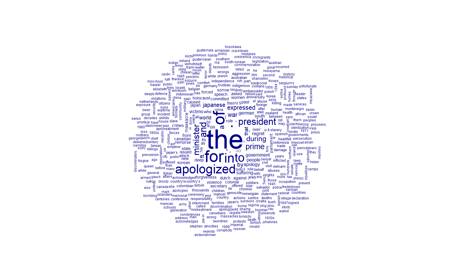
You might recall from the lecture that we need to remove certain tokens that are not useful for our analysis. Quanteda already has a list of stopwords (but you can also create your own). Let’s remove them and see what happens:
dfm_pac %>%
  dfm_remove(quanteda::stopwords("en")) %>%
  topfeatures()
Returning:
         . apologized  president   minister      prime          ,        war  expressed   japanese
       310        219        144        130        101         84         72         67         55
         "
        51
dfm_pac %>%
dfm_remove(quanteda::stopwords("en")) %>%
textplot_wordcloud()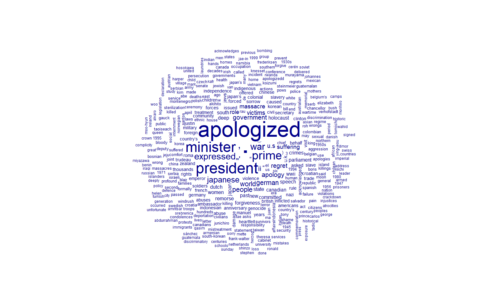
🗣️ CLASSROOM-WIDE DISCUSSION: Would you remove any other tokens? Why?
Part III - Extracting the ‘object’ of the apology (30 min)
🧑🏫 THIS IS A TEACHING MOMENT
- Discover the keywords in context function (
kwic).
Before we revisit our tokens, let’s look at an interesting feature of quanteda. We can search for a pattern (a keyword) in our corpus and see the text surrounding it using the kwic function.
For example, after reading the description of apologies, I am curious to see how words with the prefix ‘apolog-’ are used in the corpus:
quanteda::kwic(tokens_pac %>% head(n=10), pattern="apolog*")| docname | from | to | pre | keyword | post | pattern |
|---|---|---|---|---|---|---|
| 2022-07-11 NLD -> BIH.1 | 10 | 10 | Kasja Ollongren offered ’ deepest | apologies | ’ for the Dutch failure | apolog* |
| 2022-03-10 DNK -> GRL.1 | 6 | 6 | Denmark’s Prime Minister Mette Frederiksen | apologized | in person to six surviving | apolog* |
| 2022-02-17 NLD -> IDN.1 | 7 | 7 | Prime Minister Mark Rutte offered | apologies | for systematic and excessive violence | apolog* |
| 2021-12-13 CAN -> CAN.1 | 4 | 4 | Canada’s defence minister | apologized | to victims of sexual assault | apolog* |
| 2021-11-27 NLD -> NLD.1 | 5 | 5 | Dutch minister Van Engelshoven | apologized | on behalf of the Dutch | apolog* |
| 2021-11-25 SVK -> SVK.1 | 4 | 4 | The Slovakian government | apologized | to the thousands of Roma | apolog* |
(Your class teacher will explain what * in the pattern="apolog*" parameter does)
In sum, the above is an example of a regular expression (regex), a language just for expressing patterns of strings. You can read more about regex in Chapter 15 of R for Data Science 2nd edition book
kwic
Let’s try to make this data more interesting for further analysis. In the following steps, we will:
- use the power of
kwicto try to extract just the object of the apology - build a new corpus out of this new subset of text data
- remove unnecessary tokens (stop words + punctuation)
- A closer look at the output of
kwic. Pay close attention to the columns produced after running this function. Ah, this time, we increased thewindowof tokens that show up before and after the keyword:
quanteda::kwic(tokens_pac %>% head(n=10), pattern="apolog*", window=40) %>% as.data.frame()| docname | from | to | pre | keyword | post | pattern |
|---|---|---|---|---|---|---|
| 2022-07-11 NLD -> BIH.1 | 10 | 10 | Dutch Minister of Defence Kasja Ollongren offered ’ deepest | apologies | ’ for the Dutch failure to protect the victims of the Srebrenica Genocide . | apolog* |
| 2022-03-10 DNK -> GRL.1 | 6 | 6 | Denmark’s Prime Minister Mette Frederiksen | apologized | in person to six surviving Greenlandic Inuit who were taken from their families as children . | apolog* |
| 2022-02-17 NLD -> IDN.1 | 7 | 7 | Dutch Prime Minister Mark Rutte offered | apologies | for systematic and excessive violence in Indonesia’s 1945-49 war of independence . | apolog* |
| 2021-12-13 CAN -> CAN.1 | 4 | 4 | Canada’s defence minister | apologized | to victims of sexual assault , misconduct and discrimination in the military | apolog* |
| 2021-11-27 NLD -> NLD.1 | 5 | 5 | Dutch minister Van Engelshoven | apologized | on behalf of the Dutch government to the transgender community for forced sterilization of transgenders who wished to receive sex-change surgery . | apolog* |
| 2021-11-25 SVK -> SVK.1 | 4 | 4 | The Slovakian government | apologized | to the thousands of Roma women who have been forcibly sterilized . | apolog* |
Note: the info we care about the most is the column post - it contains the text immediately after a match.
This is good, but there is a downside to the keyword we used. Not all entries have the term apolog* in their description. You can confirm that by comparing dim(df_pac) with kwic(tokens_pac, pattern="apolog*", window=40). Whereas the original data set had 396 records, the kwic output has only 270.
- Try adding a more complex pattern. Here, we combine multiple keywords using the
|operator. This means we are looking for any of the keywords in the pattern.
df_kwic <-
  quanteda::kwic(tokens_pac,
                 pattern="apolog*|regre*|sorrow*|recogni*|around*|sorry*|remorse*|failur*",
                 window=40) %>%
  as.data.frame()
dim(df_kwic)
[1] 355 7We still seem to be losing some documents, but we are getting closer to what we want.
💡 Take a look at View(df_kwic)
- Handling duplicates Some rows are repeated because of multiple pattern matches in the same text:
df_kwic %>% group_by(docname) %>% filter(n() > 1)| docname | from | to | pre | keyword | post | pattern |
|---|---|---|---|---|---|---|
| 2022-07-11 NLD -> BIH.1 | 10 | 10 | Dutch Minister of Defence Kasja Ollongren offered ’ deepest | apologies | ’ for the Dutch failure to protect the victims of the Srebrenica Genocide . | apolog|regre|sorrow|recogni|around|sorry|remorse|failur |
| 2022-07-11 NLD -> BIH.1 | 15 | 15 | Dutch Minister of Defence Kasja Ollongren offered ’ deepest apologies ’ for the Dutch | failure | to protect the victims of the Srebrenica Genocide . | apolog|regre|sorrow|recogni|around|sorry|remorse|failur |
| 2020-11-30 NLD -> NLD.1 | 4 | 4 | The Dutch government | apologized | to transgender people for previously mandating surgeries , including sterilization , as a prerequisite for legal gender recognition . | apolog|regre|sorrow|recogni|around|sorry|remorse|failur |
| 2020-11-30 NLD -> NLD.1 | 22 | 22 | The Dutch government apologized to transgender people for previously mandating surgeries , including sterilization , as a prerequisite for legal gender | recognition | . | apolog|regre|sorrow|recogni|around|sorry|remorse|failur |
| 2017-12-20 MEX -> MEX.1 | 4 | 4 | The Mexican government | apologized | to three hñähñú indigenous women and recognized that it unfairly imprisoned them for 3 years . | apolog|regre|sorrow|recogni|around|sorry|remorse|failur |
| 2017-12-20 MEX -> MEX.1 | 11 | 11 | The Mexican government apologized to three hñähñú indigenous women and | recognized | that it unfairly imprisoned them for 3 years . | apolog|regre|sorrow|recogni|around|sorry|remorse|failur |
Here is how we will deal with these duplicates: let’s keep the one with the longest post text. This is equivalent to selecting the one with the earliest from value in the dataframe above.
df_kwic <- df_kwic %>% arrange(from) %>% group_by(docname) %>% slice(1)
dim(df_kwic)
[1] 336 7
Note: This is a choice! There is no absolute objective way to handle this case. Would you do anything differently?
🏠 TAKE-HOME (OPTIONAL) ACTIVITY: We used to have 367 rows, but now we have 336. How would you change the pattern to avoid excluding data from the original data frame? (Note: I do not have a ready solution to this! Feel free to share yours on #help-labs)
- Go back to pre-processing the data. Now that we have a new dataframe, we can create a more robust workflow: produce a new corpus, handle the tokens, create a dfm (bag of words), convert it to a TF-IDF matrix, and plot a wordcloud:
corp_pac <- corpus(df_kwic, text_field="post", docid_field="docname")

my_stopwords <- c(stopwords("en"))

tokens_pac <-
  # Get rid of punctuations
  tokens(corp_pac, remove_punct = TRUE) %>%
  # Get rid of stopwords
  tokens_remove(pattern = my_stopwords) %>%
  # Use multiple ngrams
  # The tokens will be concatenated by "_"
  tokens_ngrams(n=1:3)

# Try to run the code below with and without the `dfm_tfidf` function
dfm_pac <- dfm(tokens_pac) # %>% dfm_tfidf()
textplot_wordcloud(dfm_pac)
dfm_pac %>% topfeatures()Returning:
         war        world    world_war       people           ii       war_ii world_war_ii
          55           34           32           30           28           27           27
     victims     massacre    suffering
          25           24           22
🗣️ CLASSROOM DISCUSSIONS:
- In what ways is the wordcloud above fundamentally different from the one we did before?
- Do you sense a theme in the words above? What is it?
Part IV. Dimensionality Reduction + Clustering (30 min)
You will likely not have time to finish this section in class. If that is the case, you can finish it at home. If any questions arise outside of class, please use the #help-labs channel on Slack.
Instead of running k-means or any other clustering algorithm on the full dfm, let’s reduce the number of features of our dataset. This would save storage and make the process run faster.
🎯 ACTION POINTS
- You know about PCA - we’ve been playing with this linear dimensionality reduction technique for a while now. We want to show you an alternative method called Latent Sentiment Analysis (LSA) this time. The linear algebra behind it is a bit more complex, but the idea is the same: we want to reduce the number of features (words) in our dataset to just a few dimensions - even if that comes with the cost of losing some interpretability.
One of the quanteda packages has a function called textmodel_lsa that does this for us. We will use it to reduce the number of features to 3 dimensions:
df_lsa <- quanteda.textmodels::textmodel_lsa(dfm_pac %>% dfm_tfdif(), nd=3)$docs %>% as.data.frame()

head(df_lsa)| V1 | V2 | V3 | |
|---|---|---|---|
| 1957-01-01 JPN -> AUS.1 | 0.0003039 | 0.0054509 | -0.0000578 |
| 1957-01-01 JPN -> MMR.1 | 0.0047189 | 0.0364113 | -0.0013458 |
| 1965-06-22 JPN -> KOR.1 | 0.0066562 | 0.0540788 | 0.0018270 |
| 1974-04-09 PAK -> BGD.1 | 0.0341532 | 0.0040371 | 0.0067429 |
| 1982-08-26 JPN -> Transnational.1 | 0.0103963 | 0.0883948 | -0.0068312 |
| 1984-09-06 JPN -> KOR.1 | 0.0001728 | 0.0048123 | -0.0002918 |
- Visualise it. Let’s plot the first 3 dimensions of the LSA output:
# Let's treat you to an interactive plot, while we are at it:
plot_ly(data =  bind_cols(df_lsa, df_kwic),
        x = ~V1,
        y = ~V2,
        z = ~V3,
        size = 3,
        alpha = 0.7,
        type="scatter3d",
        mode="markers",
        text=~paste('Doc ID:', docname))
- Investigate the clear outlier:
# Search for this entry in the original data frame
df_pac %>%
        filter(apology_id == "1995-07-01 JPN -> *Transnational*") %>%
        pull(description) %>%
        print()
[1] "Japanese Prime Minister Tomiichi Murayama apologized to the roughly 200,000 women who were put into brothels by Japanese forces to serve as sex slaves or “comfort women” and sets up a private “Asian Women’s Fund” to deal with reparations. "- How many clusters are there in this dataset? Here is a new trick for you: the
NbClustpackage. It implements 30 indices for determining the number of clusters in a dataset and offers a voting system to decide the best number. This makes it a little less subjective than the elbow method.
res.nbclust <- df_lsa %>% select(V1, V2, V3) %>%
    scale() %>%
    # You can change the distance metric here
    NbClust(distance = "euclidean",
            min.nc = 2, max.nc = 10,
            method = "complete", index ="all")
The indices have voted! They say the best number of clusters is 4.
- Apply topic modelling. Instead of k-means, we will use another unsupervised technique called topic modelling. As the name implies, this clustering technique is more suitable for text data. The most popular of such families of models is called Latent Dirichlet Allocation (LDA). We will not go into how it works, but you can read more about it here.
tmod_lda <- topicmodels::LDA(dfm_pac %>% dfm_subset(ntoken(dfm_pac) > 0), k = 4)

## What are the topics mostly associated with each cluster?
tmod_lda %>% topicmodels::terms(10)
Assign each row to a topic:
df_topics <- tmod_lda %>% topicmodels::topics() %>% as.data.frame()
# Fix data types
df_topics <- tibble::rownames_to_column(df_topics, "docname")
colnames(df_topics) <- c("docname", "topic")
df_topics$topic <- as.factor(df_topics$topic)

df_kwic <- left_join(df_kwic, df_topics, by="docname")
Let’s plot the clusters. This time, I’m adding the post column to the tooltip so you can read the description of each apology:
# Thanks, ChatGPT, for providing the regex below!
# It breaks the text into lines of 30 characters
# but avoids breaking words in the middle
better_tooltip <-
        paste('Doc ID:',
              df_kwic$docname,
              '\nDescription:\n',
              str_replace_all(df_kwic$post, "(.{1,30})(\\s|$)", "\\1\n"))

plot_ly(data =  bind_cols(df_lsa, df_kwic),
        x = ~V1,
        y = ~V2,
        z=~V3,
        size = 3,
        color = ~topic,
        type="scatter3d",
        mode="markers",
        text=better_tooltip)
🤔 It looks like the 3D representation does not truly encapsulate the topics/clusters in the same region of the space. Why do you think that is?
- Which tokens best describe each cluster? Let’s use the
textstat_keynessfunction to find out:
We can use the concept of keyness to score words in relation to a target vs a reference group. Read more about keyness here.
# Change the cluster number to see the results for each cluster
selected_cluster = 1

tstat_key <- textstat_keyness(dfm_pac,
                              measure="chi",
                              target = case_when(is.na(df_kwic$topic) ~ FALSE,
                                                 df_kwic$topic == selected_cluster ~ TRUE,
                                                 .default = FALSE))
textplot_keyness(tstat_key, labelsize=2)
Plot a word cloud with just the target group:
textplot_wordcloud(tstat_key, comparison=FALSE, min_count=2)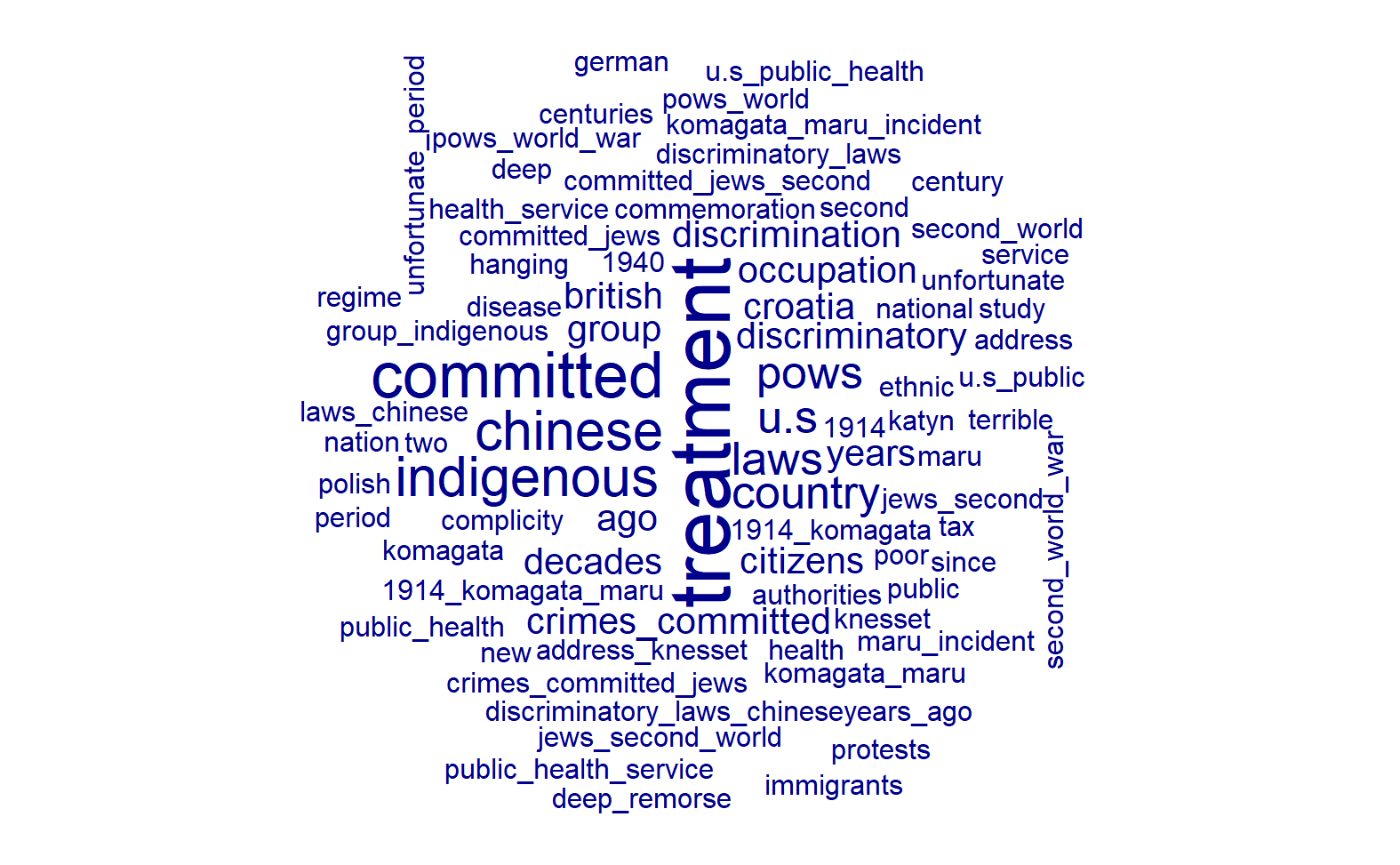
Wordcloud to compare target vs reference:
textplot_wordcloud(tstat_key, comparison=TRUE, min_count=2)
–
🗣️ CLASSROOM DISCUSSIONS
This is your last DS202W lab! Take some time to reflect on how the text mining application we did today encapsulates many of the main concepts we have learned in this course.
Before you say goodbye to your classmates and teacher, discuss the following questions:
- Why do you think we deliberately showed you new dimensionality reduction (LSA) and clustering techniques (LDA) today? Why not just stick to PCA and k-means?
- Why do you think there are so many clustering techniques out there? See, for example, this table from the Python library, scikit-learn.
- Would you use any of the techniques we learned today in your own research? Why or why not?
Footnotes
We’re gonna cry a little bit, not gonna lie. But no hard feelings. We’ll get over it.↩︎