✅ Week 08 - Lab Solutions

Comparing models and model evaluation

Author

Dr Stuart Bramwell and Dr Ghita Berrada

Instead of just reading the solutions, you might want to download the .qmd file and run the code yourself. You can download the .qmd file by clicking on the download button below:

⚙️ Setup

Import required libraries:

# Tidyverse packages we will use
library(ggplot2)
library(dplyr)     
library(tidyr)     
library(readr)     

# Tidymodel packages we will use
library(rsample)
library(yardstick) 
library(parsnip)   
library(recipes)   
library(workflows) 
library(rpart)
library(rpart.plot)
library(tune)
library(randomForest)
library(vip)
# New packages for SVM
library(LiblineaR)
library(kernlab)

Read the data set:

It is the dataset you’ve downloaded last week.

# Modify the filepath if needed
filepath <- "data/corruption_data_2019_nomissing.csv"
corruption_data_2019 <- read_csv(filepath)

🧑‍🏫 TEACHING MOMENT:

(Your class teacher will guide you through this section. Just run all the code chunks below together with your class teacher.)

🎯 ACTION POINTS:

Create the corruption_poor column by running the following code.

corruption_data_2019 <- 
  corruption_data_2019 %>% 
  mutate(corruption_poor = if_else(cpi_score < 50, "poor", "not poor"),
         corruption_poor = as.factor(corruption_poor))

Select the columns we will use to analyse the data.


corruption_data_2019 <- 
  corruption_data_2019 %>% 
  select(corruption_poor, property_rights:education_index)

Let’s again randomly split our dataset into a training set (containing 70% of the rows in our data) and a test set (including 30% of the rows in our data), and retrieve our resulting training and testing sets.

set.seed(123)
# Randomly split the initial data frame into training and testing sets (70% and 30% of rows, respectively)
split <- initial_split(corruption_data_2019, prop = 0.7, strata = corruption_poor)
training_data <- training(split)
testing_data <- testing(split)

Just like in last week’s lab, we use stratified cross-validation (i.e a cross-validation procedure where we ensure that, for each fold, both training and test sets have the feature of interest - in our example feature corruption_poor- sampled in the same proportion as in the original dataset). Stratified cross-validation is particularly useful in case of class imbalance to ensure that all classes in the data are represented appropriately during the training procedure and to make sure there is no fold where one of the classes we’re trying to predict is not sampled at all!

Create a recipe, a decision tree model specification, and wrap them up into a workflow.

In this decision tree specification, we’re tuning the min_n hyperparameter (i.e a parameter that refers to the minimum number of observations required in a terminal (leaf) node).

# Create a recipe
cpi_rec <-
  recipe(corruption_poor ~ .,
         data = training_data)

# Create the specification of a model
dt_spec <- 
    decision_tree(mode = "classification", 
    # You must specify the parameter you want to tune
    min_n = tune()) %>% 
    set_engine("rpart")

wflow <- 
  workflow() %>% 
  add_recipe(cpi_rec) %>% 
  add_model(dt_spec)

The bias-variance tradeoff is an essential concept to consider when choosing a model. Bias is a concept describing the difference between the model’s average prediction and the expected value. A model with high bias is said to be underfitting to the data. It makes simplistic assumptions about the training data, which makes it difficult to learn the underlying pattern. Variance captures the generalisability of the model. High variance typically means that we are overfitting to our training data, finding patterns and complexity that are a product of randomness as opposed to some real trend. Ideally, we are looking for a model with low bias, and low variance.

In order to understand the bias-variance tradeoff, we will be varying a hyperparameter of the decision tree to produce more complex decision tree models for comparison. We will do this using the tune_grid() function from the tune package, which uses grid search to train different models based on the parameter values you have chosen. The hyperparameter we are varying here is the min_n - a parameter that refers to the minimum number of observations required in a terminal (leaf) node.

set.seed(234)
folds <- vfold_cv(training_data, v = 5)

ctrl <- control_grid(verbose = FALSE, save_pred = TRUE)

# Create a grid specifying the min number we want to try
grid_search <- expand_grid(
  min_n = c(3:8)
)

# This will take a little while
dt_res <- tune_grid(
  wflow,
  # This computes k-fold CV during tuning
  resamples = folds,
  grid = grid_search,
  # Making sure we keep the out-of-sample predictions for each resample during tuning
  control = control_grid(verbose = FALSE, save_pred = TRUE)
)

If we want to find out which parameter created the best model, we can run the following command.

show_best(dt_res, metric = "roc_auc")


# A tibble: 5 × 7
  min_n .metric .estimator  mean     n std_err .config              
  <int> <chr>   <chr>      <dbl> <int>   <dbl> <chr>                
1     8 roc_auc binary     0.949     5  0.0105 Preprocessor1_Model07
2     9 roc_auc binary     0.949     5  0.0105 Preprocessor1_Model08
3    10 roc_auc binary     0.949     5  0.0105 Preprocessor1_Model09
4    14 roc_auc binary     0.927     5  0.0371 Preprocessor1_Model13
5    15 roc_auc binary     0.927     5  0.0371 Preprocessor1_Model14

Plot the values for the roc_auc metric for each value of min_n we have tried with the grid search.

g <- dt_res %>% autoplot(metric="roc_auc")

# Customise the look of the plot
g + 
  theme_bw(base_size=20) + 
  labs(y = "ROC-AUC" , title="Decision Tree performance (training set)") +
  ylim(0.8, 1) +  
  scale_x_continuous(breaks = seq(2, 15, 1))

Note that we set the y-scale of our AUC curve plot as [0.8-1] to better visualise the fluctuations of AUC as the min_n hyperparameter varies: AUC values don’t below 0.8 for decision tree models on the training dataset (as specified above) regardless of min_n value. To make the rest of the AUC plots comparable to this one, we’ll be using the same y-scale for all AUC plots from now on.

Now visualise the out-of-sample predictions for each value of min_n we have tried - e.g. the average validation set predictions.

g <- 
  collect_predictions(dt_res)  %>%
  group_by(min_n) %>%
  roc_auc(truth=corruption_poor, .pred_poor, event_level="second") %>% # Remember to set event_level="second" (predicted class = poor)
  ggplot() +
  geom_point(aes(x=min_n, y=.estimate)) +
  geom_line(aes(x=min_n, y=.estimate))

# Customise the look of the plot
g + 
  theme_bw(base_size=20) + 
  labs(y = "ROC-AUC", title="Decision Tree performance (test set)") +
  ylim(0.8, 1) + 
  scale_x_continuous(breaks = seq(2, 15, 1))

🗣️ DISCUSSION:

We trained different models using a variety of values for our min_n parameter. Looking at the training vs testing performance at each value, how do you think the parameter changes the overfitting or underfitting of the model?

Part II - Comparing models (30 min)

🧑‍🏫 TEACHING MOMENT: Your class teacher will briefly explain the concept of decision boundaries and how different models produce different decision boundaries.

So far we have looked at decision trees. But how well do other models compare to predicting a country’s level of corruption?

Create a new recipe, model specification, and workflow for the support vector machine model. Note that this is using a linear kernel, SVM models can also be used with polynomial, radial and sigmoid kernels.

# SVMs do not accept NAs or categorical variables
# Create the specification of a support vector machine (SVM) model
# SVMs do not accept NAs or categorical variables
# Create the specification of a support vector machine (SVM) model
cpi_rec <-
  recipe(corruption_poor ~ ., data = training_data) %>%
  # What if there are missing values? We input the missing values using the k-nearest neighbors algorithm
  step_impute_knn(all_predictors(), neighbors = 3)

# Create the specification of a support vector machine (SVM) model
svm_spec <- 
  svm_linear(mode = "classification") %>%
  set_engine("LiblineaR")

wflow_svm <- 
  workflow() %>% 
  add_recipe(cpi_rec) %>% 
  add_model(svm_spec)

Have a look at the recipe here: it includes a rather unfamiliar step step_impute_knn. What does that correspond to? Your data could contain missing values (and the test data actually does in the education_index column!). Instead of potentially distorting the distribution of the data by simply removing the missing values, we perform missing value imputation, i.e we’re trying to estimate the values of the blanks.

One of the methods for doing this is the k-nearest neighbours method, which estimates missing values based on the characteristics of similar neighboring data points. In practice, this means that:

the subset of data points that have non-missing values for the target variable are identified (i.e if the target variable is education_index , the subset of data points which have a value for education_index are identified)

calculate the Euclidean distance between the data point with the missing value and each data point in the subset that was identified in the previous step. The Euclidean distance calculation ignores the feature that has a missing value and only uses the features that have complete values (e.g if education_index is the feature with missing value, education_index is not taken into account in the Euclidean distance calculations)

select the K closest neighbours (K is a parameter passed to the imputation algorithm and gives the number of neighbours to take into account in the final calculation) based on the Euclidean distance previously calculated.

The final imputed value is obtained as follows:

\[ x_j=\frac{\sum_{i=1}^K w_i v_i}{\sum_{i=1}^K w_i} \]

where

\[ \begin{split} &K \quad \text{number of neighbours} \\ &w_i \quad \text{Euclidian distance between i-th number and data point with missing value}\\ &v_i \quad \text{value of feature containing missing value in i-th neighbour} \end{split} \]

The step_impute_knn step performs (as you can expect from the name), k-nearest neighbour imputation (also abbreviated as KNN imputation). And in our case, we choose K to be 3 and choose to impute all predictors, i.e to try and estimate missing values in all predictor columns.

Now that you have a workflow to fit an SVM model:

Fit the model to a testing and training set, calculating an appropriate metric (e.g. confusion matrix, ROC/AUC curve). How does it compare to the decision tree?


model <- 
  wflow_svm %>% 
  fit(training_data)

model %>% 
  augment(new_data = cpi_rec %>% bake(testing_data)) %>% 
  f_meas(truth = corruption_poor, estimate = .pred_class)

# A tibble: 1 × 3
  .metric .estimator .estimate
  <chr>   <chr>          <dbl>
1 f_meas  binary         0.857

Train an SVM model, using a radial kernel.

svm_spec <- 
  svm_rbf() %>%
  set_mode("classification") %>% 
  set_engine("kernlab")

wflow_svm <- 
  workflow() %>% 
  add_recipe(cpi_rec) %>% 
  add_model(svm_spec)

model <- 
  wflow_svm %>% 
  fit(training_data)

model %>% 
  augment(new_data = testing_data) %>% 
  f_meas(truth = corruption_poor, estimate = .pred_class)

# A tibble: 1 × 3
  .metric .estimator .estimate
  <chr>   <chr>          <dbl>
1 f_meas  binary         0.867

Part III - Ensemble methods (40 min)

🧑‍🏫 TEACHING MOMENT: Your class teacher will briefly explain the concept of ensemble methods.

While we can tweak hyperparameters to reduce overfitting and underfitting to try and improve the bias-variance tradeoff in decision trees, we also have techniques such as ‘ensemble methods’ which can also help to improve modelling results. Ensemble learning helps to improve predictions by combining several models, which can lead to better predictive performance than compared to a single model. The basic idea is to learn a set of classifiers (experts) and to allow them to vote.

Ensemble algorithms, such as bootstrapping aggregation (bagging) and boosting, which aim to reduce variance at the small cost of bias in decision trees.

We suggest you have these tabs open in your browser:

The tidymodels documentation page (you can open tabs with documentation pages for each package if you need to)
The tidyverse documentation page (you can open tabs with documentation pages for each package if you need to)

This is a model specification for boosting decision trees (this one is for XGBoost).

boost_spec <- boost_tree(trees = 200, tree_depth = 4) %>%
  set_engine("xgboost") %>%
  set_mode("classification")

Apply boosting to our dataset using a workflow.

{r}
cpi_rec <-
  recipe(corruption_poor ~ .,
         data = training_data) %>%
  step_dummy(all_nominal_predictors(), one_hot = TRUE) 


wflow_boost <- 
  workflow() %>% 
  add_recipe(cpi_rec) %>% 
  add_model(boost_spec)

boost_model <- 
  wflow_boost %>% 
  fit(data = training_data)

boost_model %>% 
  augment(training_data) %>%
  conf_mat(truth = corruption_poor, .pred_class) %>%
  autoplot(type = "heatmap")

No false positives or false negatives on the training dataset: this classifier looks like a “perfect” one!

boost_model %>% 
  augment(testing_data) %>%
  conf_mat(truth = corruption_poor, .pred_class) %>%
  autoplot(type = "heatmap")

On the test set, the performance degrades slightly as expected but the performance remains rather good overall. Note that this classifier seems to do slightly worse in terms of false negatives than in terms of false positives i.e it tends to misclassify countries with poor corruption record as not having a poor record more than it misclassifies countries with a good record of corruption as having a bad corruption record : given the application domain, this could be rather problematic (after all, detecting instances of bad practice is more important than the contrary!).

How does this compare to decision trees?
Tune the hyperparameters using a grid search to improve your model.

 {r}
 rec_boost <-
  recipe(corruption_poor ~ .,
         data = training_data) %>%
  step_dummy(all_nominal_predictors(), one_hot = TRUE)

# Add the tune() function to the parameter you want to tune
boost_spec <- 
  boost_tree(trees = tune(), tree_depth = 4) %>%
  set_engine("xgboost") %>%
  set_mode("classification")

wflow_boost <- 
  workflow() %>% 
  add_recipe(rec_boost) %>% 
  add_model(boost_spec)

set.seed(234)
folds <- vfold_cv(training_data, v = 5,strata=corruption_poor)

ctrl <- control_grid(verbose = FALSE, save_pred = TRUE)

# Create a grid specifying the min number we want to try
grid_search = expand_grid(
  trees = floor(seq(1, 30, length.out = 5))
)

# This will take a little while
boost_res <- tune_grid(
  wflow_boost,
  resamples = folds,
  grid = grid_search,
  control = ctrl
)

g <- boost_res %>% autoplot(metric="roc_auc")

# Customise the look of the plot
g + 
  theme_bw(base_size=20) + 
  labs(y = "ROC-AUC") +
  ylim(0.8, 1) + 
  scale_x_continuous(breaks = floor(seq(1, 30, length.out = 5)))

# Show best model
show_best(boost_res)

# A tibble: 5 × 7
  trees .metric .estimator  mean     n std_err .config             
  <dbl> <chr>   <chr>      <dbl> <int>   <dbl> <chr>               
1  8.25 roc_auc binary     1         5 0       Preprocessor1_Model2
2 15.5  roc_auc binary     1         5 0       Preprocessor1_Model3
3 22.8  roc_auc binary     1         5 0       Preprocessor1_Model4
4 30    roc_auc binary     0.998     5 0.00220 Preprocessor1_Model5
5  1    roc_auc binary     0.957     5 0.0168  Preprocessor1_Model1

As expected, boosted trees consistently outperform decision trees: a plateau of AUC performance (AUC of 1 based on cross-validation results!) is reached for a number of trees set between 8 and 22, with the value of AUC slightly dipping when the number of trees is either set to 1 (0.957) or 30 (0.998) but remaining above the best AUC value achieved by the decision tree model (AUC of 0.949 for tree numbers set 8, 9 or 10).

# The model with the best performing value of n can be selected using select_best()
best_complexity <- select_best(boost_res)
boost_final <- finalize_workflow(wflow_boost, best_complexity)
boost_final

According to the documentation, the select_best function “inds the tuning parameter combination with the best performance values” (here, performance is measured in terms of AUC) and we then use the finalize_workflow function to update our original workflow to use this new optimal model.

══ Workflow ════════════════════════════════════════════════════════════════════════════════════════════════════════════════════════════════════════════════════════════════════════════════════════
Preprocessor: Recipe
Model: boost_tree()

── Preprocessor ────────────────────────────────────────────────────────────────────────────────────────────────────────────────────────────────────────────────────────────────────────────────────
1 Recipe Step

• step_dummy()

── Model ───────────────────────────────────────────────────────────────────────────────────────────────────────────────────────────────────────────────────────────────────────────────────────────
Boosted Tree Model Specification (classification)

Main Arguments:
  trees = 8.25
  tree_depth = 4

Computational engine: xgboost

boost_final_fit <- fit(boost_final, data = training_data)
boost_final_fit

══ Workflow [trained] ══════════════════════════════════════════════════════════════════════════════════════════════════════════════════════════════════════════════════════════════════════════════
Preprocessor: Recipe
Model: boost_tree()

── Preprocessor ────────────────────────────────────────────────────────────────────────────────────────────────────────────────────────────────────────────────────────────────────────────────────
1 Recipe Step

• step_dummy()

── Model ───────────────────────────────────────────────────────────────────────────────────────────────────────────────────────────────────────────────────────────────────────────────────────────
##### xgb.Booster
raw: 10.9 Kb 
call:
  xgboost::xgb.train(params = list(eta = 0.3, max_depth = 4, gamma = 0, 
    colsample_bytree = 1, colsample_bynode = 1, min_child_weight = 1, 
    subsample = 1), data = x$data, nrounds = 8.25, watchlist = x$watchlist, 
    verbose = 0, nthread = 1, objective = "binary:logistic")
params (as set within xgb.train):
  eta = "0.3", max_depth = "4", gamma = "0", colsample_bytree = "1", colsample_bynode = "1", min_child_weight = "1", subsample = "1", nthread = "1", objective = "binary:logistic", validate_parameters = "TRUE"
xgb.attributes:
  niter
callbacks:
  cb.evaluation.log()
# of features: 13 
niter: 8.25
nfeatures : 13 
evaluation_log:
    iter training_logloss
       1       0.48118032
       2       0.34716195
---                      
       7       0.11335254
       8       0.09502884

(Bonus)

Apply bagging to decision trees to try and reduce overfitting. Can you also do it while tuning hyperparameters?

cpi_rec <-
  recipe(corruption_poor ~ .,
         data = training_data) %>%
  step_dummy(all_nominal_predictors(), one_hot = TRUE) %>%
  step_impute_knn(all_predictors(),skip=FALSE)

  # Create the specification of a model
bagging_spec <- 
   rand_forest(mtry = .cols()) %>%
  set_engine("randomForest", importance = TRUE) %>%
  set_mode("classification")

wflow_forest <- 
  workflow() %>% 
  add_recipe(cpi_rec) %>% 
  add_model(bagging_spec)

random_forest_model <- 
  wflow_forest %>% 
  fit(data = training_data)

# Evaluate the fitted random forest model using confusion matrices & summary stats
conf_mat_training <- random_forest_model %>% 
  augment(training_data) %>%
  conf_mat(truth = corruption_poor, .pred_class) 

conf_mat_training %>%
  summary()

conf_mat_training %>%
  autoplot(type = "heatmap")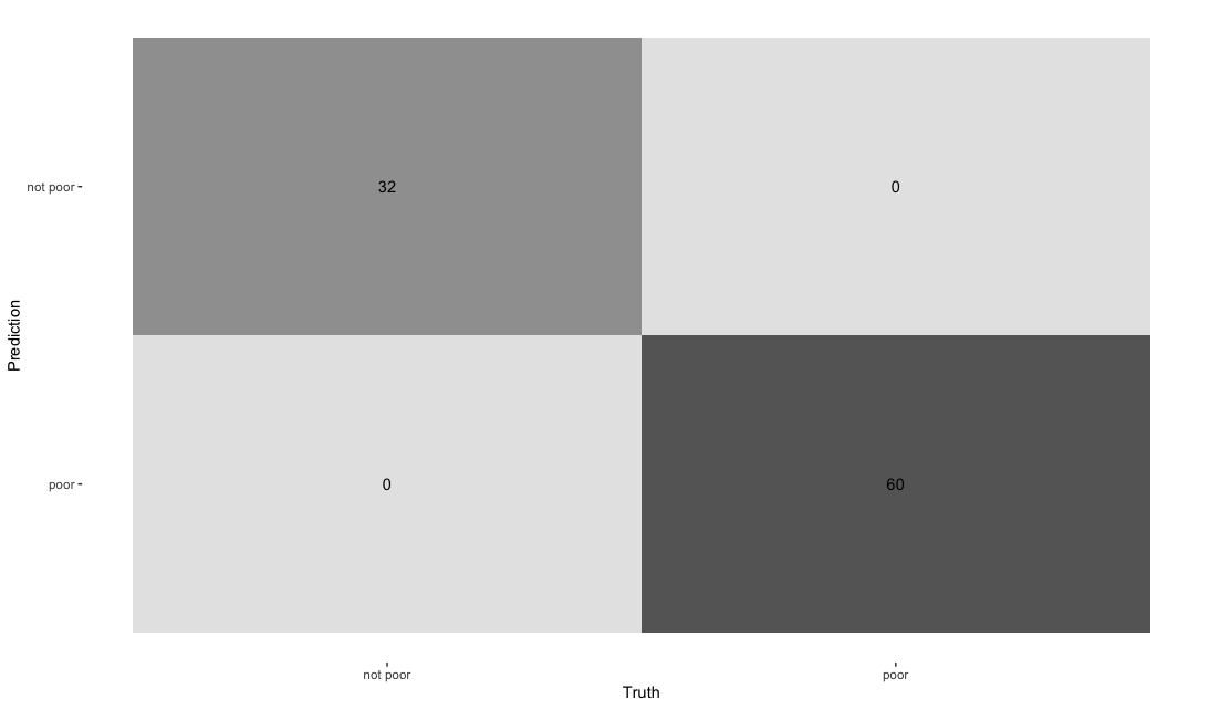

# A tibble: 13 × 3
   .metric              .estimator .estimate
   <chr>                <chr>          <dbl>
 1 accuracy             binary         1    
 2 kap                  binary         1    
 3 sens                 binary         1    
 4 spec                 binary         1    
 5 ppv                  binary         1    
 6 npv                  binary         1    
 7 mcc                  binary         1    
 8 j_index              binary         1    
 9 bal_accuracy         binary         1    
10 detection_prevalence binary         0.348
11 precision            binary         1    
12 recall               binary         1    
13 f_meas               binary         1

conf_mat_testing <- random_forest_model %>% 
  augment(testing_data) %>%
  conf_mat(truth = corruption_poor, .pred_class) 

conf_mat_testing %>% summary()

conf_mat_testing %>% autoplot(type = "heatmap")

# A tibble: 13 × 3
   .metric              .estimator .estimate
   <chr>                <chr>          <dbl>
 1 accuracy             binary         0.905
 2 kap                  binary         0.793
 3 sens                 binary         0.867
 4 spec                 binary         0.926
 5 ppv                  binary         0.867
 6 npv                  binary         0.926
 7 mcc                  binary         0.793
 8 j_index              binary         0.793
 9 bal_accuracy         binary         0.896
10 detection_prevalence binary         0.357
11 precision            binary         0.867
12 recall               binary         0.867
13 f_meas               binary         0.867

What if we now tune the hyperparameters trees and min_n?

tune_spec <- rand_forest(
  mtry = 13,
  trees = tune(),
  min_n = tune()
) %>%
  set_mode("classification") %>%
  set_engine("randomForest", importance=TRUE)

tune_wf <- workflow() %>%
  add_recipe(cpi_rec) %>%
  add_model(tune_spec)

set.seed(456)
folds <- vfold_cv(training_data, v = 5, strata=corruption_poor)

ctrl <- control_grid(verbose = FALSE, save_pred = TRUE)

# Create a grid specifying the min number we want to try
grid_search = expand_grid(
  trees = seq(1,25, length.out = 5),
  min_n = seq(1,20)
)

# This will take a little while
rand_res <- tune_grid(
  tune_wf,
  resamples = folds,
  grid = grid_search,
  control = ctrl
)

g <- rand_res %>% autoplot(metric="roc_auc")

# Customise the look of the plot
g + 
  theme_bw(base_size=20) + 
  theme(legend.position = "right") + 
  labs(y = "ROC-AUC") +
  ylim(0.8, 1) + 
  scale_x_continuous(breaks = seq(0,20, 2), limits = c(1, 20))

# Show best model
show_best(rand_res)

> show_best(rand_res)
# A tibble: 5 × 8
  trees min_n .metric .estimator  mean     n std_err .config               
  <dbl> <int> <chr>   <chr>      <dbl> <int>   <dbl> <chr>                 
1    13     2 roc_auc binary     0.983     2 0.00458 Preprocessor1_Model042
2    13     5 roc_auc binary     0.981     2 0.0192  Preprocessor1_Model045
3    13    12 roc_auc binary     0.978     2 0.0220  Preprocessor1_Model052
4    25     7 roc_auc binary     0.978     2 0.0220  Preprocessor1_Model087
5    25    13 roc_auc binary     0.978     2 0.0220  Preprocessor1_Model093

Based on these metrics, random forest comes second best after boosted trees and before decision trees for this particular data set…

# The model with the best performing value of n can be selected using select_best()
best_complexity <- select_best(rand_res, metric="roc_auc")
rand_final <- finalize_workflow(tune_wf, best_complexity)
rand_final_fit <- fit(rand_final, data = training_data)

rand_final

 rand_final
══ Workflow ════════════════════════════════════════════════════════════════════════════════════════════════════════════════════════════════════════════════════════════════════════════════════════════════════
Preprocessor: Recipe
Model: rand_forest()

── Preprocessor ────────────────────────────────────────────────────────────────────────────────────────────────────────────────────────────────────────────────────────────────────────────────────────────────
2 Recipe Steps

• step_dummy()
• step_naomit()

── Model ───────────────────────────────────────────────────────────────────────────────────────────────────────────────────────────────────────────────────────────────────────────────────────────────────────
Random Forest Model Specification (classification)

Main Arguments:
  mtry = 13
  trees = 13
  min_n = 2

Engine-Specific Arguments:
  importance = TRUE

Computational engine: randomForest

rand_final_fit

══ Workflow [trained] ══════════════════════════════════════════════════════════════════════════════════════════════════════════════════════════════════════════════════════════════════════════════════════════
Preprocessor: Recipe
Model: rand_forest()

── Preprocessor ────────────────────────────────────────────────────────────────────────────────────────────────────────────────────────────────────────────────────────────────────────────────────────────────
2 Recipe Steps

• step_dummy()
• step_naomit()

── Model ───────────────────────────────────────────────────────────────────────────────────────────────────────────────────────────────────────────────────────────────────────────────────────────────────────

Call:
 randomForest(x = maybe_data_frame(x), y = y, ntree = ~13, mtry = min_cols(~13,      x), nodesize = min_rows(~2L, x), importance = ~TRUE) 
               Type of random forest: classification
                     Number of trees: 13
No. of variables tried at each split: 13

        OOB estimate of  error rate: 5.43%
Confusion matrix:
         not poor poor class.error
not poor       30    2      0.0625
poor            3   57      0.0500