
✅ Week 07 Lab - Solutions
Decision trees with tidymodels
Instead of just reading the solutions, you might want to download the .qmd file and run the code yourself. You can download the .qmd file by clicking on the download button below:
📋 Lab Tasks
⚙️ Setup
Import required libraries:
# Tidyverse packages we will use
library(dplyr)
library(tidyr)
library(readr)
library(stringr)

# Tidymodel packages we will use
library(yardstick)
library(parsnip)
library(recipes)
library(workflows)
library(rpart)
library(rsample)
library(tune)
library(rpart.plot)
library(vip)
library(ggplot2)
Read the 2019 data set:
It is the first brand-new dataset you’ve downloaded.
# Modify the filepath if needed
filepath <- "data/corruption_data_2019_nomissing.csv"
corruption_data_2019 <- read_csv(filepath)
Rows: 140 Columns: 105
── Column specification ────────────────────────────────────────────────────────────────────────────────────────────────────────────────────────────────────────────
Delimiter: ","
chr (6): country_code, economy, region, income_group, getting_electricity_s...
dbl (99): db_year, starting_a_business_procedures_men_number, starting_a_bus...
ℹ Use `spec()` to retrieve the full column specification for this data.
ℹ Specify the column types or set `show_col_types = FALSE` to quiet this message.We’ve been doing a lot of training vs testing splits in this course, primarily by hand and focused on a particular point in time (e.g., test samples are defined to start in 2019).
But not all splits need to be done this way. Some data sets don’t have a time-series component and can be split randomly for testing purposes. To make things more robust, we don’t just simply use one single train versus test split, but we use a technique called cross-validation and split the data into multiple train vs test splits.
In this lab, we’ll learn how to use cross-validation to build a more robust model for changes in the data. Let’s kick things off by cleaning up our data and randomly splitting it into a training set (70% of data points/rows) and a test set (30% of data points/rows).
🧑🏫 TEACHING MOMENT:
(Your class teacher will guide you through this section. Just run all the code chunks below together with your class teacher.)
Our goal in this lab is to predict the level of corruption in a given country. The Corruption Perception Index (CPI), already present in our data set (in the cpi_score column), sorts countries according to their perceived corruption levels. According to (Lima and Delen 2020),“[t]he index captures the assessments of domain experts on corrupt behavioral information, originating a scale from 0 to 100 where economies close to 0 are perceived as highly corrupt while economies close to 100 are perceived as less corrupt”. In other words, the CPI already gives us a way to classify countries in scales of corruption. To go from a scale of 0 to 100 (which is the CPI scale), to a categorical variable (which is what we need for our classification), we simply need the following definition:
Corruption class: We define the following levels of corruption based on the CPI scale:
- if the CPI is lower than 50, then the corruption level is
poor - if the CPI is between 50 (included) and 70 (excluded), then the corruption level is
average - if the CPI is higher than 70, then the corruption level is
good
We store the result in the
corruption_classcolumn- if the CPI is lower than 50, then the corruption level is
Convert the
corruption_classcolumn from character to factor
🎯 ACTION POINTS:
- Create the
corruption_classcolumn and convert it tofactor.
corruption_data_2019 <- corruption_data_2019 %>%
  mutate(corruption_class = case_when(
    cpi_score < 50 ~ "poor",
    50 <= cpi_score & cpi_score < 70 ~ "average",
    cpi_score >=70 ~ "good") %>% as.factor())
An equivalent code chunk is the following:
corruption_data_2019 <- corruption_data_2019 %>%
                     mutate(corruption_class = case_when(
                        cpi_score < 50 ~ "poor" ,
                        50<= cpi_score & cpi_score < 70 ~ "average" ,
                        cpi_score >= 70 ~ "good")
                     )
corruption_data_2019$corruption_class <- as.factor(corruption_data_2019$corruption_class)
To check the result of what we’ve done, let’s print the first ten rows of the cpi_score and newly-created corruption_class columns:
  corruption_data_2019 %>%
       select(cpi_score,corruption_class)%>%
       head(10)
# A tibble: 10 × 2
   cpi_score corruption_class
       <dbl> <fct>
 1        16 poor
 2        35 poor
 3        35 poor
 4        26 poor
 5        45 poor
 6        42 poor
 7        77 good
 8        77 good
 9        30 poor
10        26 poor
- Now, let’s randomly split our dataset into a training set (containing 70% of the rows in our data) and a test set (including 30% of the rows in our data)
#Randomly split the initial data frame into training and testing sets (70% and 30% of rows, respectively)
split <- initial_split(corruption_data_2019, prop = 0.7)
What is in the training and testing set?
To get the actual data assigned to either set, use the
rsample::training()andrsample::testing()functions:
training_data <- training(split)
testing_data <- testing(split)
For curiosity, let’s confirm which unique countries are represented in our training and test sets and by how many data points. We can uncover this mystery by counting the unique values in the economy column (you could do the same per region).
# tallying the number of rows per country in the training set
training_data %>%
    group_by(economy) %>%
    tally()
# A tibble: 98 × 2
economy n
<chr> <int>
1 Afghanistan 1
2 Argentina 1
3 Armenia 1
4 Australia 1
5 Bangladesh 1
6 Barbados 1
7 Belarus 1
8 Benin 1
9 Bolivia 1
10 Brazil 1
# ℹ 88 more rows
# ℹ Use `print(n = ...)` to see more rows# tallying the number of rows per country in the test set
testing_data %>%
group_by(economy) %>%
tally()# A tibble: 42 × 2
economy n
<chr> <int>
1 Albania 1
2 Algeria 1
3 Angola 1
4 Austria 1
5 Azerbaijan 1
6 Belgium 1
7 Bhutan 1
8 Bosnia and Herzegovina 1
9 Botswana 1
10 Cabo Verde 1
# ℹ 32 more rows
# ℹ Use `print(n = ...)` to see more rowsThe result here is not particularly illuminating as each country is only represented only once in our training or test data set. No country present in the training set is present in the test set.
Just how many non-empty records are there in our datasets per country?
# tallying the number of non-empty rows per country in the training set
training_data %>%
    drop_na() %>%
    group_by(economy) %>%
    tally() %>%
    knitr::kable()
|economy | n|
|:------------------------|--:|
|Afghanistan | 1|
|Argentina | 1|
|Armenia | 1|
|Australia | 1|
|Bangladesh | 1|
|Barbados | 1|
|Belarus | 1|
|Benin | 1|
|Brazil | 1|
|Brunei Darussalam | 1|
|Bulgaria | 1|
|Burkina Faso | 1|
|Burundi | 1|
|Cambodia | 1|
|Cameroon | 1|
|Central African Republic | 1|
|Chad | 1|
|Chile | 1|
|China | 1|
|Comoros | 1|
|Costa Rica | 1|
|Croatia | 1|
|Cyprus | 1|
|Denmark | 1|
|Djibouti | 1|
|Dominican Republic | 1|
|El Salvador | 1|
|Equatorial Guinea | 1|
|Estonia | 1|
|Ethiopia | 1|
|Finland | 1|
|France | 1|
|Gabon | 1|
|Georgia | 1|
|Germany | 1|
|Greece | 1|
|Guatemala | 1|
|Guinea | 1|
|Guyana | 1|
|Hungary | 1|
|Iceland | 1|
|Ireland | 1|
|Italy | 1|
|Jordan | 1|
|Kazakhstan | 1|
|Kenya | 1|
|Lesotho | 1|
|Luxembourg | 1|
|Malawi | 1|
|Maldives | 1|
|Mali | 1|
|Mauritius | 1|
|Mongolia | 1|
|Morocco | 1|
|Mozambique | 1|
|Nepal | 1|
|Netherlands | 1|
|Nicaragua | 1|
|Nigeria | 1|
|Norway | 1|
|Oman | 1|
|Pakistan | 1|
|Papua New Guinea | 1|
|Paraguay | 1|
|Peru | 1|
|Philippines | 1|
|Poland | 1|
|Portugal | 1|
|Romania | 1|
|Rwanda | 1|
|Saudi Arabia | 1|
|Serbia | 1|
|Seychelles | 1|
|Sierra Leone | 1|
|Slovenia | 1|
|Solomon Islands | 1|
|South Africa | 1|
|Spain | 1|
|Sri Lanka | 1|
|Sudan | 1|
|Sweden | 1|
|Switzerland | 1|
|Tajikistan | 1|
|Thailand | 1|
|Togo | 1|
|Tunisia | 1|
|Turkey | 1|
|Uganda | 1|
|Ukraine | 1|
|United Kingdom | 1|
|Uruguay | 1|
|Uzbekistan | 1|
|Zimbabwe | 1|# tallying the number of non-empty rows per country in the test set
testing_data %>%
drop_na() %>%
group_by(economy) %>%
tally() %>%
knitr::kable()|economy | n|
|:----------------------|--:|
|Albania | 1|
|Algeria | 1|
|Angola | 1|
|Austria | 1|
|Azerbaijan | 1|
|Belgium | 1|
|Bhutan | 1|
|Bosnia and Herzegovina | 1|
|Botswana | 1|
|Cabo Verde | 1|
|Canada | 1|
|Colombia | 1|
|Dominica | 1|
|Ecuador | 1|
|Ghana | 1|
|Haiti | 1|
|Honduras | 1|
|India | 1|
|Indonesia | 1|
|Israel | 1|
|Jamaica | 1|
|Japan | 1|
|Latvia | 1|
|Lebanon | 1|
|Liberia | 1|
|Lithuania | 1|
|Madagascar | 1|
|Malaysia | 1|
|Malta | 1|
|Mauritania | 1|
|Mexico | 1|
|Montenegro | 1|
|Namibia | 1|
|New Zealand | 1|
|Niger | 1|
|Panama | 1|
|Senegal | 1|
|Singapore | 1|
|Suriname | 1|
|Trinidad and Tobago | 1|
|Zambia | 1|But again, this was not particularly illuminating. So let’s take a slightly different approach and, instead, check which data points had missing values in our training and test sets.
Before going on a goose chase, let’s check a few things.
nrow(training_data)[1] 98training_data %>%
drop_na() %>%
tally()# A tibble: 1 × 1
n
<int>
1 93Our training data has 98 rows but only 93 of them have complete data, which means 5 rows have missing values. Which countries do these rows correspond to?
training_data %>%
         filter(if_any(everything(),is.na)) %>%
         select(economy)
# A tibble: 5 × 1
economy
<chr>
1 Moldova
2 Vietnam
3 Kosovo
4 Eswatini
5 Bolivia The same approach replicated to the test data produces the following results:
testing_data %>%
         filter(if_any(everything(),is.na)) %>%
         select(economy)
# A tibble: 1 × 1
economy
<chr>
1 TanzaniaIf interested, you can replicate the same analysis we just did by region instead of by economy (i.e by country).
training_data %>%
    group_by(region) %>%
    tally()
# A tibble: 7 × 2
region n
<chr> <int>
1 East Asia & Pacific 9
2 Europe & Central Asia 15
3 High income: OECD 22
4 Latin America & Caribbean 13
5 Middle East & North Africa 6
6 South Asia 6
7 Sub-Saharan Africa 27testing_data %>%
group_by(region) %>%
tally()# A tibble: 7 × 2
region n
<chr> <int>
1 East Asia & Pacific 3
2 Europe & Central Asia 4
3 High income: OECD 8
4 Latin America & Caribbean 10
5 Middle East & North Africa 3
6 South Asia 2
7 Sub-Saharan Africa 12# tallying the number of non-empty rows per region in the training set
training_data %>%
drop_na() %>%
group_by(region) %>%
tally() %>%
knitr::kable()|region | n|
|:--------------------------|--:|
|East Asia & Pacific | 8|
|Europe & Central Asia | 13|
|High income: OECD | 22|
|Latin America & Caribbean | 12|
|Middle East & North Africa | 6|
|South Asia | 6|
|Sub-Saharan Africa | 26|# tallying the number of non-empty rows per region in the test set
testing_data %>%
drop_na() %>%
group_by(region) %>%
tally() %>%
knitr::kable()|region | n|
|:--------------------------|--:|
|East Asia & Pacific | 3|
|Europe & Central Asia | 4|
|High income: OECD | 8|
|Latin America & Caribbean | 10|
|Middle East & North Africa | 3|
|South Asia | 2|
|Sub-Saharan Africa | 11|To browse the original Ease of Doing Business dataset, including a description of the variables (though some were recoded for ease of comprehension) - included in the Metadata sheet of the file-, you can download the Excel file below:
For more information about other variables of the dataset (i.e variables related to the Economic Freedom Index, Education Index or CPI), check out the explanations in (Lima and Delen 2020).
🗣️ DISCUSSION:
We defined corruption (and corruption levels) in a specific way, and we will be building a model to predict corruption in a way that fits this definition. Do you think that the definition we gave of corruption is satisfactory? Is it a good modelling objective? If not, what would you do differently? (You can look at the dataset documentation for further ideas).
Part II - Introduction to decision trees (40 min)
🧑🏻🏫 TEACHING MOMENT: In this part, you’ll be learning about a new classification model called decision trees, which is more suited to handle large numbers of features of varying types that potentially contain missing data than logistic regression.
Our dataset is a real-world dataset and ticks all these boxes:
- We mentioned earlier that our goal is to build a model to predict
corruption_class. Aside from a few variables that don’t look like likely predictors (e.g.db_year,economy,region,income_group(though this one is debatable),cpi_score(it is correlated with the outcome variable so can’t be used to predict it!)), we have a large potential number of features/predictors to choose from for our model (100! for a dataset that only has 140 rows/data points). - Many variables include missing values
- Though we smoothed things out, the various variables had varying types (e.g., categorical values or strings or numerical values)
Your class teacher will explain the basic principle of a decision tree.
As usual, we start with a recipe
For computational reasons (too long to run!), we’ll be building our model with a random subset of features from the original dataset. We’ll randomly choose 25 variables from the original columns of the dataset, excluding the columns db_year, economy,region,income_group and cpi_score.
We construct a vector predictors, which contains the names of our chosen predictors:
  remove <- c("country_code","economy","region","income_group","db_year","cpi_score","corruption_class") # list of the columns we exclude
  predictors <- corruption_data_2019 %>%
                colnames() %>%
                str_remove_all(., paste(remove, collapse = "|"))%>%
                .[!(.=="")] %>%
                sample(.,25)
Since we’re selecting a random sample of predictors, we print the predictors we currently use in our model.
predictors %>%
         knitr::kable()
|x |
|:-----------------------------------------------------------------------------------------------------|
|paying_taxes_time_hours_per_year |
|registering_property_procedures_number |
|paying_taxes_labor_tax_and_contributions_percent_of_profit |
|protecting_minority_investors_strength_of_minority_investor_protection_index_0_50_db15_20_methodology |
|paying_taxes_profit_tax_percent_of_profit |
|registering_property_equal_access_to_property_rights_index_2_0_db17_20_methodology |
|property_rights |
|getting_electricity_mechanisms_for_restoring_service_0_1_db16_20_methodology |
|trading_across_borders_time_to_export_documentary_compliance_hours_db16_20_methodology |
|education_index |
|enforcing_contracts_trial_and_judgment_days |
|labor_freedom |
|enforcing_contracts_enforcement_of_judgment_days |
|trade_freedom |
|government_spending |
|fiscal_health |
|enforcing_contracts_attorney_fees_percent_of_claim |
|dealing_with_construction_permits_building_quality_control_index_0_15_db16_20_methodology |
|getting_credit_credit_bureau_coverage_percent_of_adults |
|dealing_with_construction_permits_quality_control_after_construction_index_0_3_db16_20_methodology |
|registering_property_transparency_of_information_index_0_6_db17_20_methodology |
|enforcing_contracts_alternative_dispute_resolution_0_3_db17_20_methodology |
|protecting_minority_investors_extent_of_disclosure_index_0_10 |
|protecting_minority_investors_extent_of_corporate_transparency_index_0_7_db15_20_methodology |
|registering_property_time_days |Then, we write our recipe:
formula_string <- paste("corruption_class ~", paste(predictors, collapse = " + "))
formula <- as.formula(formula_string)
impute_rec <- recipe(formula, data = training_data) %>%
  step_impute_median(all_numeric(), -all_outcomes()) %>%
  prep()
Here, the only pre-processing step we perform before fitting our model is a simple median imputation in order to fill in missing values (in numeric columns) per column with the median value of their respective column.
Let’s check what our recipe is like:
print(impute_rec)── Recipe ───────────────────────────────────────────────────────────────────────────────────────────────────────────────────────────────────────────────────────────────────────────────────────────
── Inputs
Number of variables by role
outcome: 1
predictor: 25
── Training information
Training data contained 98 data points and 5 incomplete rows.
── Operations
• Median imputation for: paying_taxes_time_hours_per_year, registering_property_procedures_number, paying_taxes_labor_tax_and_contributions_percent_of_profit, ... | TrainedNow, we can fit a decision tree model on our data
You can create the model specification for a decision tree using this scaffolding code (you need to install the rpart library using the install.packages("rpart") command to be able to use this code and of course, load the rpart library):
# Create the specification of a model but don't fit it yet
dt_spec <- decision_tree(mode = "classification", tree_depth = 5) %>%
  set_engine("rpart")
What if we, again, print our tree specification?
print(dt_spec)Decision Tree Model Specification (classification)
Main Arguments:
tree_depth = 5
Computational engine: rpartNow that you have the model specification:
- Fit the model to the training set using a workflow and evaluate it its performance with an appropriate metric (e.g AUC/ROC curve)
We first fit the model to the training set using a workflow:
#Delete this line and write your code here
wflow <-
  workflow() %>%
  add_recipe(impute_rec) %>%
  add_model(dt_spec)

model <-
  wflow %>%
  fit(data = training_data)

fitted_model <- model %>% extract_fit_parsnip()
We evaluate the performance of the model using several metrics (confusion matrix, AUC/ROC curve, metrics summary)
model %>%
  augment(new_data = bake(impute_rec, training_data)) %>%
  select(corruption_class:.pred_poor) %>%
  conf_mat(estimate = .pred_class, truth = corruption_class) %>%
  autoplot(type = "heatmap")
model %>%
  augment(new_data = bake(impute_rec, training_data)) %>%
  select(corruption_class:.pred_poor) %>%
  roc_auc(.pred_poor,.pred_average,.pred_good, truth = corruption_class)
# A tibble: 1 × 3
.metric .estimator .estimate
<chr> <chr> <dbl>
1 roc_auc hand_till 0.227model %>%
augment(new_data = bake(impute_rec, training_data)) %>%
select(corruption_class:.pred_poor) %>%
roc_curve(.pred_poor,.pred_average,.pred_good, truth = corruption_class) %>%
autoplot()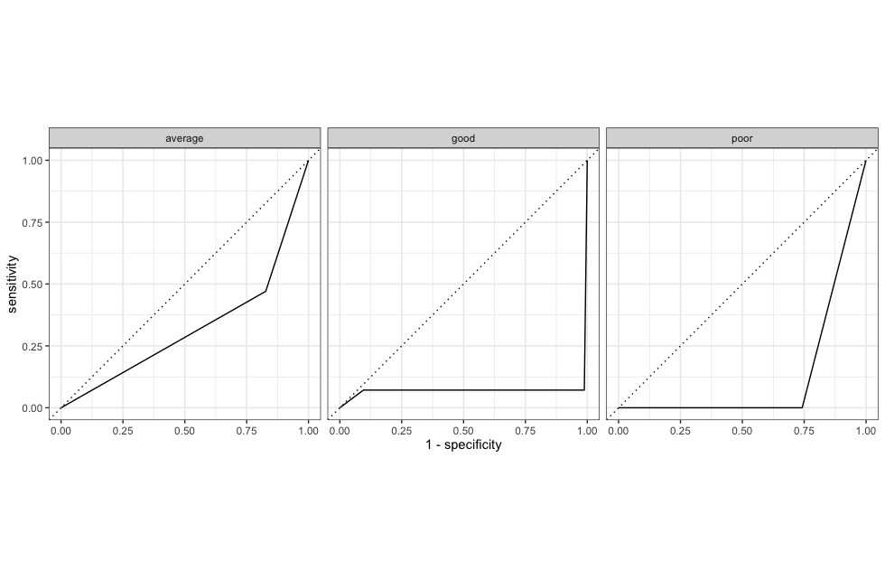
model %>%
  augment(new_data = bake(impute_rec, training_data)) %>%
  conf_mat(estimate = .pred_class, truth = corruption_class) %>%
  summary()
# A tibble: 13 × 3
.metric .estimator .estimate
<chr> <chr> <dbl>
1 accuracy multiclass 0.898
2 kap multiclass 0.768
3 sens macro 0.800
4 spec macro 0.906
5 ppv macro 0.904
6 npv macro 0.962
7 mcc multiclass 0.785
8 j_index macro 0.706
9 bal_accuracy macro 0.853
10 detection_prevalence macro 0.333
11 precision macro 0.904
12 recall macro 0.800
13 f_meas macro 0.829Note that our dataset has class imbalance:
corruption_data_2019 %>%
  group_by(corruption_class) %>%
  summarise(n = n()) %>%
  mutate(Freq = n/sum(n))
# A tibble: 3 × 3
corruption_class n Freq
<fct> <int> <dbl>
1 average 27 0.193
2 good 20 0.143
3 poor 93 0.664(The class poor is much more frequent than the other two classes).
So, metrics like accuracy are not exactly suited to evaluate the performance of our model properly! Balanced accuracy or F1-score are more appropriate.
Based on most metrics, our tree seems to perform decently well but the AUC metric paints a widely different picture! This could be due to our (arbitrary) selection of features!
- Fit the model to the test set using a workflow and evaluate its performance with an appropriate metric (e.g AUC/ROC curve)
model %>%
  augment(new_data = bake(impute_rec, testing_data)) %>%
  select(corruption_class:.pred_poor) %>%
  conf_mat(estimate = .pred_class, truth = corruption_class) %>%
  autoplot(type = "heatmap")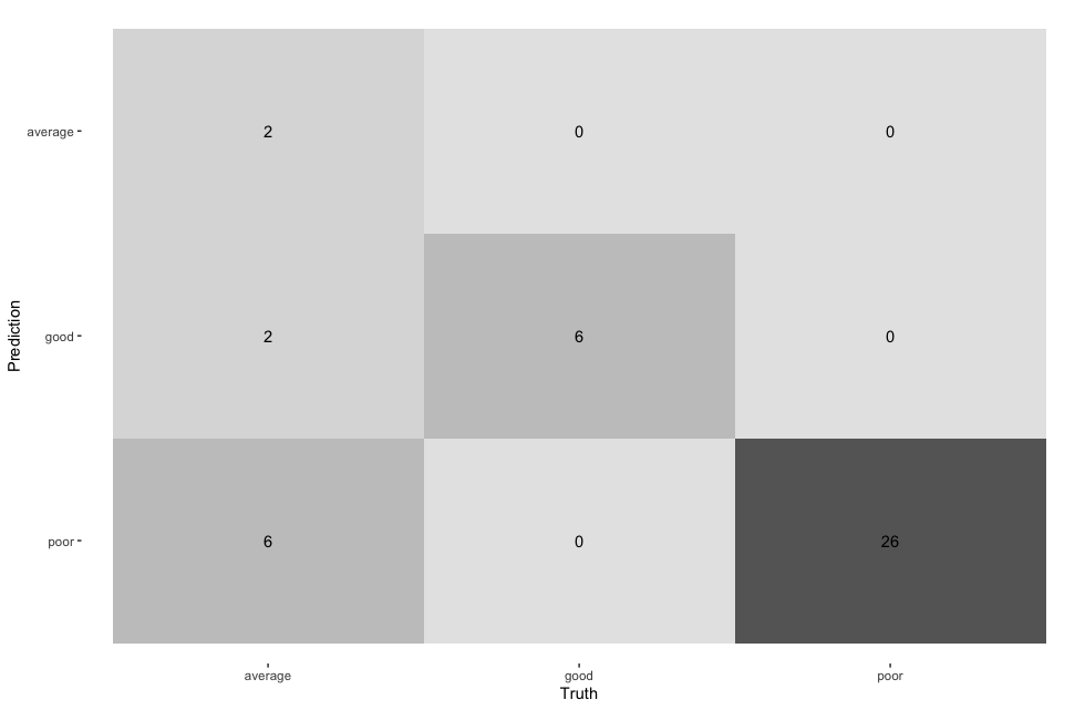
model %>%
  augment(new_data = bake(impute_rec, testing_data)) %>%
  select(corruption_class:.pred_poor) %>%
  roc_auc(.pred_poor,.pred_average,.pred_good, truth = corruption_class)
# A tibble: 1 × 3
.metric .estimator .estimate
<chr> <chr> <dbl>
1 roc_auc hand_till 0.25model %>%
augment(new_data = bake(impute_rec, testing_data)) %>%
select(corruption_class:.pred_poor) %>%
roc_curve(.pred_poor,.pred_average,.pred_good, truth = corruption_class) %>%
autoplot()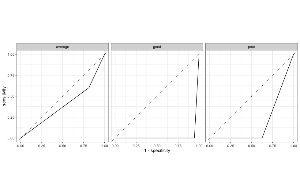
model %>%
  augment(new_data = bake(impute_rec, testing_data)) %>%
  conf_mat(estimate = .pred_class, truth = corruption_class) %>%
  summary()
# A tibble: 13 × 3
.metric .estimator .estimate
<chr> <chr> <dbl>
1 accuracy multiclass 0.810
2 kap multiclass 0.611
3 sens macro 0.733
4 spec macro 0.856
5 ppv macro 0.854
6 npv macro 0.933
7 mcc multiclass 0.660
8 j_index macro 0.590
9 bal_accuracy macro 0.795
10 detection_prevalence macro 0.333
11 precision macro 0.854
12 recall macro 0.733
13 f_meas macro 0.696Bonus
Here’s what this tree looks like:
tree_fit <- model %>% extract_fit_engine()
rpart.plot(tree_fit,roundint=FALSE)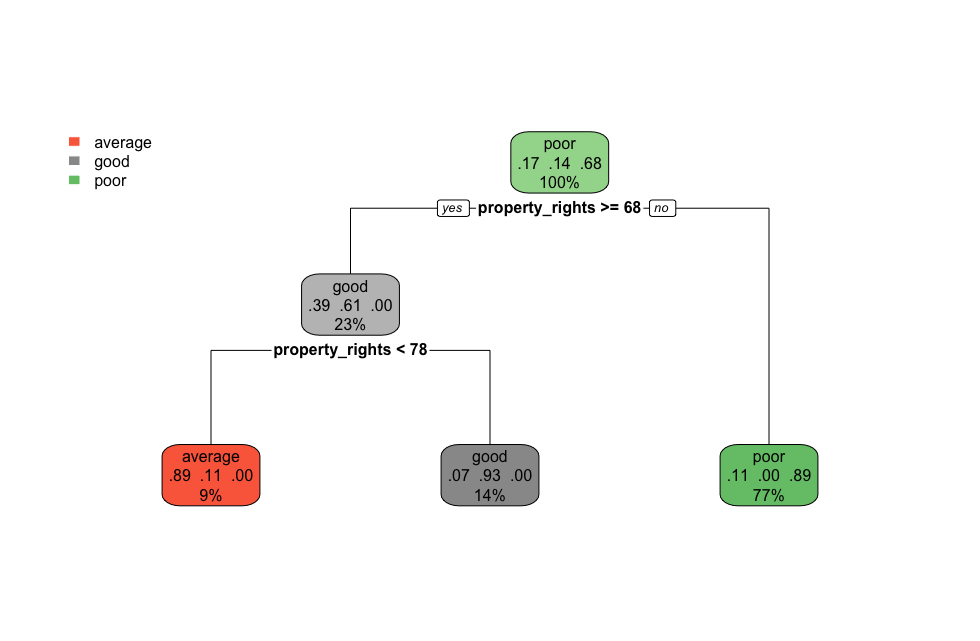
And here are its features ranked by importance:
tree_fit %>%
  vip(geom = "col", aesthetics = list(fill = "midnightblue", alpha = 0.8)) +
  scale_y_continuous(expand = c(0, 0))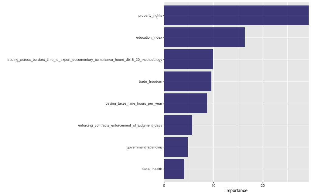
On the basis of the performance of our model on the test data, it seems that our model doesn’t generalize very well to the test data and overfitting is probable in this case. We most likely need a better way of selecting features than simply at random (and selecting an arbitrary number of them at that!)
🤔 What happens if you choose a different set of features to train your model?
We select a new set of features:
#Delete this line and write your code here
remove <- c("country_code","economy","region","income_group","db_year","cpi_score","corruption_class") # list of the columns we exclude
predictors <- corruption_data_2019 %>%
  colnames() %>%
  str_remove_all(., paste(remove, collapse = "|"))%>%
  .[!(.=="")] %>%
  sample(.,25)


predictors %>%
  knitr::kable()
|x |
|:-----------------------------------------------------------------------------------------------|
|registering_property_time_days |
|education_index |
|judicial_effectiveness |
|getting_credit_credit_registry_coverage_percent_of_adults |
|protecting_minority_investors_extent_of_ownership_and_control_index_0_7_db15_20_methodology |
|starting_a_business_cost_women_percent_of_income_per_capita |
|dealing_with_construction_permits_quality_of_building_regulations_index_0_2_db16_20_methodology |
|getting_electricity_procedures_number |
|government_integrity |
|dealing_with_construction_permits_professional_certifications_index_0_4_db16_20_methodology |
|protecting_minority_investors_extent_of_director_liability_index_0_10 |
|registering_property_quality_of_land_administration_index_0_30_db17_20_methodology |
|getting_electricity_regulatory_monitoring_0_1_db16_20_methodology |
|enforcing_contracts_alternative_dispute_resolution_0_3_db17_20_methodology |
|enforcing_contracts_attorney_fees_percent_of_claim |
|trading_across_borders_time_to_import_documentary_compliance_hours_db16_20_methodology |
|resolving_insolvency_outcome_0_as_piecemeal_sale_and_1_as_going_concern |
|resolving_insolvency_recovery_rate_cents_on_the_dollar |
|government_spending |
|trading_across_borders_cost_to_import_documentary_compliance_usd_db16_20_methodology |
|trading_across_borders_cost_to_export_border_compliance_usd_db16_20_methodology |
|trading_across_borders_time_to_export_border_compliance_hours_db16_20_methodology |
|enforcing_contracts_court_automation_0_4_db17_20_methodology |
|trade_freedom |
|property_rights |The model specification, workflow and training are the same as before:
formula_string <- paste("corruption_class ~", paste(predictors, collapse = " + "))
formula <- as.formula(formula_string)
impute_rec <- recipe(formula, data = training_data) %>%
  step_impute_median(all_numeric(), -all_outcomes()) %>%
  prep()

dt_spec <- decision_tree(mode = "classification", tree_depth = 5) %>%
  set_engine("rpart")

wflow <-
  workflow() %>%
  add_recipe(impute_rec) %>%
  add_model(dt_spec)

model <-
  wflow %>%
  fit(data = training_data)

fitted_model <- model %>% extract_fit_parsnip()
We evaluate our new model as before:
Results for training data
model %>%
  augment(new_data = bake(impute_rec, training_data)) %>%
  select(corruption_class:.pred_poor) %>%
  conf_mat(estimate = .pred_class, truth = corruption_class) %>%
  autoplot(type = "heatmap")
model %>%
  augment(new_data = bake(impute_rec, training_data)) %>%
  select(corruption_class:.pred_poor) %>%
  roc_auc(.pred_poor,.pred_average,.pred_good, truth = corruption_class)
# A tibble: 1 × 3
.metric .estimator .estimate
<chr> <chr> <dbl>
1 roc_auc hand_till 0.264model %>%
augment(new_data = bake(impute_rec, training_data)) %>%
conf_mat(estimate = .pred_class, truth = corruption_class) %>%
summary()# A tibble: 13 × 3
.metric .estimator .estimate
<chr> <chr> <dbl>
1 accuracy multiclass 0.949
2 kap multiclass 0.895
3 sens macro 0.946
4 spec macro 0.966
5 ppv macro 0.934
6 npv macro 0.960
7 mcc multiclass 0.896
8 j_index macro 0.912
9 bal_accuracy macro 0.956
10 detection_prevalence macro 0.333
11 precision macro 0.934
12 recall macro 0.946
13 f_meas macro 0.940model %>%
augment(new_data = bake(impute_rec, training_data)) %>%
select(corruption_class:.pred_poor) %>%
roc_curve(.pred_poor,.pred_average,.pred_good, truth = corruption_class) %>%
autoplot()
Results for test data
model %>%
  augment(new_data = bake(impute_rec, testing_data)) %>%
  select(corruption_class:.pred_poor) %>%
  conf_mat(estimate = .pred_class, truth = corruption_class) %>%
  autoplot(type = "heatmap")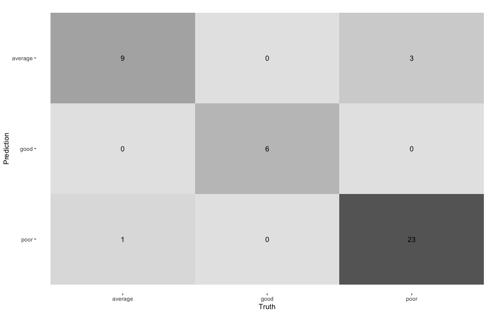
model %>%
  augment(new_data = bake(impute_rec, testing_data)) %>%
  select(corruption_class:.pred_poor) %>%
  roc_auc(.pred_poor,.pred_average,.pred_good, truth = corruption_class)
model %>%
augment(new_data = bake(impute_rec, testing_data)) %>%
select(corruption_class:.pred_poor) %>%
roc_auc(.pred_poor,.pred_average,.pred_good, truth = corruption_class)# A tibble: 1 × 3
.metric .estimator .estimate
<chr> <chr> <dbl>
1 roc_auc hand_till 0.268model %>%
augment(new_data = bake(impute_rec, testing_data)) %>%
conf_mat(estimate = .pred_class, truth = corruption_class) %>%
summary()# A tibble: 13 × 3
.metric .estimator .estimate
<chr> <chr> <dbl>
1 accuracy multiclass 0.905
2 kap multiclass 0.829
3 sens macro 0.928
4 spec macro 0.948
5 ppv macro 0.903
6 npv macro 0.933
7 mcc multiclass 0.833
8 j_index macro 0.876
9 bal_accuracy macro 0.938
10 detection_prevalence macro 0.333
11 precision macro 0.903
12 recall macro 0.928
13 f_meas macro 0.913model %>%
augment(new_data = bake(impute_rec, testing_data)) %>%
select(corruption_class:.pred_poor) %>%
roc_curve(.pred_poor,.pred_average,.pred_good, truth = corruption_class) %>%
autoplot()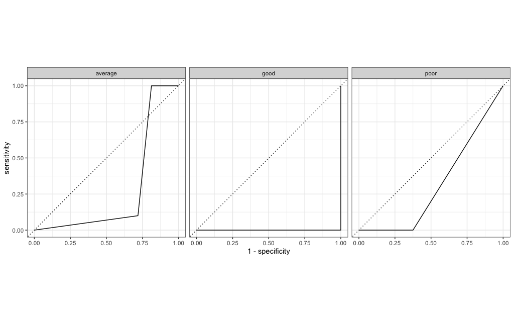
We also, as before, visualise our tree:
tree_fit <- model %>% extract_fit_engine()
rpart.plot(tree_fit,roundint=FALSE)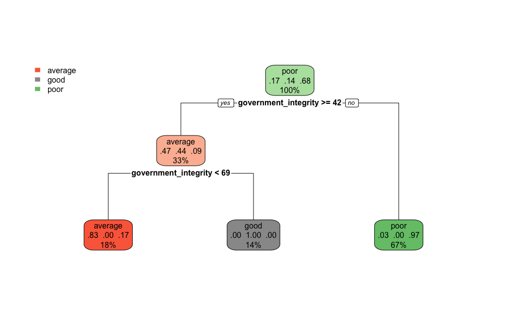
and the most important features in our model:
tree_fit %>%
  vip(geom = "col", aesthetics = list(fill = "midnightblue", alpha = 0.8)) +
  scale_y_continuous(expand = c(0, 0))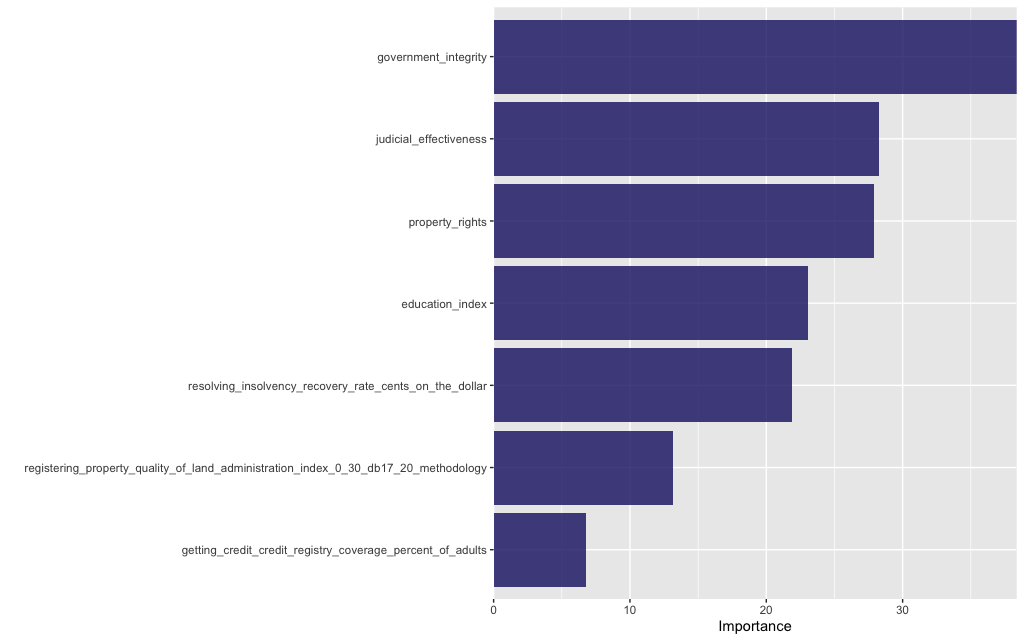
The performance of this set of features is marginally better than the previous set and more crucially it is stable between training and test sets (so this model doesn’t overfit and yields better predictions). This underlines that the choice of model features is crucial!
Part III - Cross-validation (30 min)
🧑🏻🏫 TEACHING MOMENT: Your class teacher will briefly explain the concept of cross-validation.
- Question: Can you retrain your decision tree model using cross-validation?
- Use the
initial_split()andtraining()functions to split your data and extract your training set. Documentation: rsample.
split <- initial_split(corruption_data_2019,strata=corruption_class)
# extract the training data
training_set <- training(split)- Employ a
v_fold_cv()function to the data with 10-fold cross-validation (10-fold by default).
cv <- vfold_cv(training_set, strata=corruption_class)Note that, since our data has class imbalance, we opt for 10-fold stratified cross-validation instead of simple 10-fold cross-validation to ensure that each fold contains samples of each class in the same proportion as in the original dataset (check out the stratified resampling section of this page for another explanation).
- Fit the model using
fit_resamples()and collect your metrics (as in the W05 lecture notebook). How does the model performance compare to previously?
formula_string <- paste("corruption_class ~", paste(predictors, collapse = " + "))
formula <- as.formula(formula_string)
rec <- recipe(formula, data = corruption_data_2019) %>%
  step_impute_median(all_numeric(), -all_outcomes()) %>%
  prep()

w_flow <-
  workflow() %>%
  add_recipe(rec) %>%
  add_model(dt_spec)
res <- fit_resamples(w_flow, cv) %>% collect_metrics()- What happens when you tweak tree parameters and/or cross-validation parameters?
split <- initial_split(corruption_data_2019,strata=corruption_class)
training_data <- training(split)

depth <- seq(5,20,by=5)
folds <- seq(10,30,by=10)

# Let's keep 10 folds first and let's see how varying the depth of the tree affects performance

cv <- vfold_cv(training_data, v=10, strata=corruption_class)
formula_string <- paste("corruption_class ~", paste(predictors, collapse = " + "))
formula <- as.formula(formula_string)
rec <- recipe(formula, data = corruption_data_2019) %>%
  step_impute_median(all_numeric(), -all_outcomes()) %>%
  prep()

d <- 10
# To run it once, we would write the following code:
dt_spec <-
  decision_tree(mode = "classification", tree_depth = d) %>%
  set_engine("rpart")

w_flow <-
  workflow() %>%
  add_recipe(rec) %>%
  add_model(dt_spec)
# This will take a good amount of time
fit_resamples(w_flow, cv) %>% collect_metrics() %>% mutate(depth=d)
# A tibble: 2 × 7
.metric .estimator mean n std_err .config depth
<chr> <chr> <dbl> <int> <dbl> <chr> <dbl>
1 accuracy multiclass 0.819 10 0.0213 Preprocessor1_Model1 10
2 roc_auc hand_till 0.879 10 0.0263 Preprocessor1_Model1 10# But to make it easier to re-run the same code over and over again, let's wrap it in a function
run_dt_model <- function(depth, cv){
dt_spec <-
decision_tree(mode = "classification", tree_depth = depth) %>%
set_engine("rpart")
w_flow <-
workflow() %>%
add_recipe(rec) %>%
add_model(dt_spec)
# This will take a good amount of time: go get a coffee or a tea in the meanwhile!
fit_resamples(w_flow, cv) %>% collect_metrics() %>% mutate(depth=depth)
}
# Then we can run the same code like this:
result_depth10 = run_dt_model(10, cv)
# This returned a data frame. You can run again with a different depth:
result_depth5 = run_dt_model(5, cv)
# What if I want to put all results under the same data frame? I could use dplyr::bind_rows()
bind_rows(result_depth5, result_depth10) %>% mutate(num_folds=10)
# Great, how do I automate this? With an lapply! (Elaborate: arguments to be used first, then function)
all_depths <- c(1, 5, 10, 20) # alternatively, try ALL with seq(1, 20)
final_results <- lapply(all_depths, run_dt_model,cv=cv) %>% bind_rows()
run_different_folds <- function(num_folds){
cv <- vfold_cv(training_data, v=num_folds,strata=corruption_class)
lapply(all_depths, function(depth) {run_dt_model(depth, cv)}) %>%
bind_rows() %>%
mutate(num_folds = num_folds)
}
all_folds <- c(2, 5, 10)
final_final_results <- lapply(all_folds, run_different_folds) %>% bind_rows()
# There is a simpler way of doing all of that using the rsample package! Can you figure out how to do it from the documentation??- Question: How does your model perform on (a subset of the) 2020 dataset?
filepath2020 <- "data/corruption_data_2020_nomissing.csv"
corruption_data_2020 <- read_csv(filepath2020)

corruption_data_2020 <- corruption_data_2020 %>%
  mutate(corruption_class = case_when(
    cpi_score < 50 ~ "poor",
    50 <= cpi_score & cpi_score < 70 ~ "average",
    cpi_score >=70 ~ "good") %>% as.factor())

# we select a random subset of the 2020 data
set.seed(123)
test_2020 <- corruption_data_2020 %>% sample_frac(0.42, replace = FALSE)
Here are the countries included in test_2020:
unique(test_2020$economy) %>% knitr::kable(col.names="countries")|countries |
|:-----------------|
|Benin |
|Georgia |
|Solomon Islands |
|Equatorial Guinea |
|Zimbabwe |
|Vietnam |
|Morocco |
|Mozambique |
|Uganda |
|Namibia |
|Norway |
|Latvia |
|Cameroon |
|Australia |
|El Salvador |
|Azerbaijan |
|Malta |
|Cyprus |
|Madagascar |
|Maldives |
|Uzbekistan |
|Papua New Guinea |
|Slovenia |
|Lithuania |
|Bhutan |
|Colombia |
|Philippines |
|Romania |
|Tanzania |
|Switzerland |
|Ecuador |
|Lesotho |
|Burundi |
|Canada |
|Iceland |
|Greece |
|Senegal |
|Peru |
|Poland |
|Nicaragua |
|Djibouti |
|Montenegro |
|Costa Rica |
|Nepal |
|Kazakhstan |
|Togo |
|United Kingdom |
|Ireland |
|Belgium |
|Mali |
|Cambodia |
|Oman |
|Bulgaria |
|Malawi |
|Rwanda |
|Finland |
|Seychelles |
|Bolivia |
|Armenia |model %>%
augment(new_data = bake(impute_rec, test_2020)) %>%
select(corruption_class:.pred_poor) %>%
roc_auc(.pred_poor,.pred_average,.pred_good, truth = corruption_class)# A tibble: 1 × 3
.metric .estimator .estimate
<chr> <chr> <dbl>
1 roc_auc hand_till 0.206model %>%
augment(new_data = bake(impute_rec, test_2020)) %>%
select(corruption_class:.pred_poor) %>%
roc_curve(.pred_poor,.pred_average,.pred_good, truth = corruption_class) %>%
autoplot()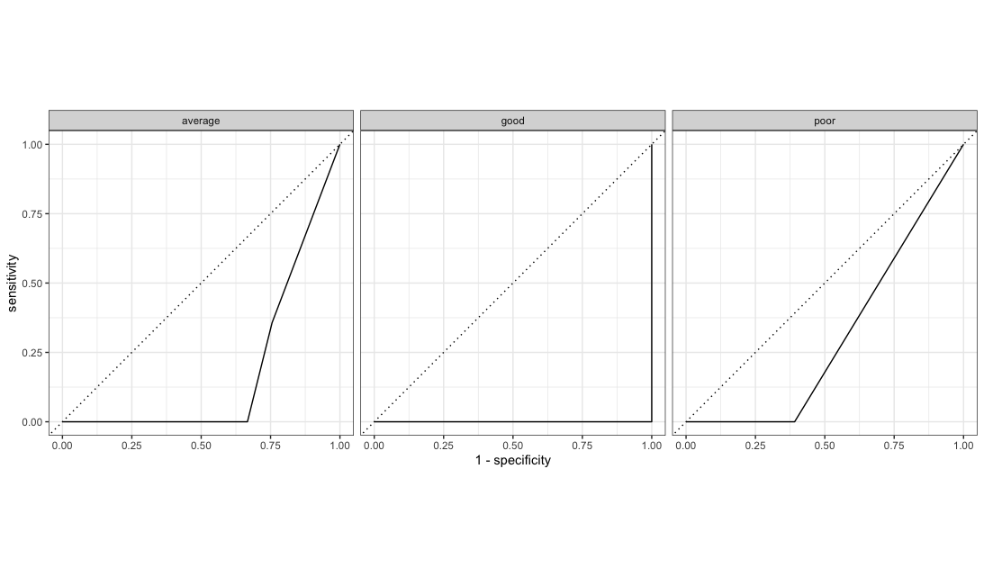
model %>%
  augment(new_data = bake(impute_rec, test_2020)) %>%
  select(corruption_class:.pred_poor) %>%
  conf_mat(estimate = .pred_class, truth = corruption_class) %>%
  autoplot(type = "heatmap")
model %>%
  augment(new_data = bake(impute_rec, test_2020)) %>%
  conf_mat(estimate = .pred_class, truth = corruption_class) %>%
  summary()
# A tibble: 13 × 3
.metric .estimator .estimate
<chr> <chr> <dbl>
1 accuracy multiclass 0.898
2 kap multiclass 0.826
3 sens macro 0.944
4 spec macro 0.956
5 ppv macro 0.9
6 npv macro 0.931
7 mcc multiclass 0.842
8 j_index macro 0.9
9 bal_accuracy macro 0.95
10 detection_prevalence macro 0.333
11 precision macro 0.9
12 recall macro 0.944
13 f_meas macro 0.911The performance deteriorates slightly on this dataset but, on the whole, this model seems to generalize relatively well and predict corruption level almost as well as on the original dataset.