✅ Week 03 Lab - Solutions

2023/24 Winter Term

Author

Instead of just reading the solutions, you might want to download the .qmd file and run the code yourself. You can download the .qmd file by clicking on the download button below:

⚙️ Setup

Import required libraries:

# Remember to install.packages() any missing packages using the Console
library(dplyr)
library(readr)
library(lubridate)
library(tidymodels)

Read the data set:

It is the same data set you used in the previous lab:

# Modify the filepath if needed
filepath <- "data/UK-HPI-full-file-2023-06.csv"
uk_hpi <- read_csv(filepath)

Rows: 136935 Columns: 54                                                                                                                                                         
── Column specification ──────────────────────────────────────────────────────────────────────────────────────────────────────────────────────
Delimiter: ","
chr  (3): Date, RegionName, AreaCode
dbl (51): AveragePrice, Index, IndexSA, 1m%Change, 12m%Change, AveragePriceSA, SalesVolume, DetachedPrice, DetachedIndex, Detached1m%Chang...

ℹ Use `spec()` to retrieve the full column specification for this data.
ℹ Specify the column types or set `show_col_types = FALSE` to quiet this message.

Pre-process the dataset:

# Replicate roughly the same steps you did in the previous lab:

# 1. Select the columns you need
# 2. Rename the columns
# 3. Filter the data set to include only the regions you need (let's focus on England for now)
# 4. Preprocess the date column

selected_cols    <- c("Date", "RegionName", "1m%Change", "SalesVolume")
df_england <-
    uk_hpi %>%
    select(all_of(selected_cols)) %>%
    rename(date = Date, region = RegionName, monthlyChangeHPI = `1m%Change`) %>%
    filter(region == "England") %>%
    drop_na(monthlyChangeHPI) %>% 
    mutate(date = lubridate::dmy(date)) %>% 
    arrange(desc(date))
df_england  %>% head(8) %>% knitr::kable()

date	region	monthlyChangeHPI	SalesVolume
2023-06-01	England	0.9	NA
2023-05-01	England	-0.1	NA
2023-04-01	England	0.4	29344
2023-03-01	England	-1.0	41065
2023-02-01	England	-0.5	39675
2023-01-01	England	-0.8	41771
2022-12-01	England	-0.7	56883
2022-11-01	England	0.4	65287

📋 Lab Tasks

Part I - the `lm` command (25 min)

👨🏻‍🏫 TEACHING MOMENT: Your class teacher will demonstrate how to run the lm function.

Task 1: Run a linear regression model with yearly_change as the dependent variable and yearly_change_lag1 as the independent variable. Save the model as model1.

model1 <- lm(SalesVolume ~ monthlyChangeHPI, data = df_england)

Print the model summary:

summary(model1)

Call:
lm(formula = SalesVolume ~ monthlyChangeHPI, data = df_england)

Residuals:
   Min     1Q Median     3Q    Max 
-44887 -11960   -548  12247  47019 

Coefficients:
                 Estimate Std. Error t value Pr(>|t|)    
(Intercept)       69427.6     1108.9   62.61   <2e-16 ***
monthlyChangeHPI  12008.9      943.6   12.73   <2e-16 ***
---
Signif. codes:  0 ‘***’ 0.001 ‘**’ 0.01 ‘*’ 0.05 ‘.’ 0.1 ‘ ’ 1

Residual standard error: 18300 on 337 degrees of freedom
  (323 observations deleted due to missingness)
Multiple R-squared:  0.3246,    Adjusted R-squared:  0.3226 
F-statistic:   162 on 1 and 337 DF,  p-value: < 2.2e-16

🗣️ DISCUSSION:

What is the value of the intercept?

\(\approx 69427.6\)

What is the value of the slope?

\(\approx 12008.9\)

How should you interpret this model?

This model suggests that whenever the house prices index increases by 1 percentage point on a period of one month (this corresponds to our monthlyChangeHPI independent variable), then the sales volume (this corresponds to our SalesVolume dependent variable) increases by a factor of 12008 approximately.

If the model is a good fit, we can also expect the slope to be correct within a 95% confidence interval of 12008.9 +/- 943.6 (given by the Std. Error of the slope coefficient).

👨🏻‍🏫 TEACHING MOMENT: Your class teacher will demonstrate how to plot the model.

Task 2: Plot the residuals against the fitted values.

plot(model1, 1)

Alternatively, see all four basic lm diagnostic plots:

par(mfrow = c(2, 2))
plot(model1)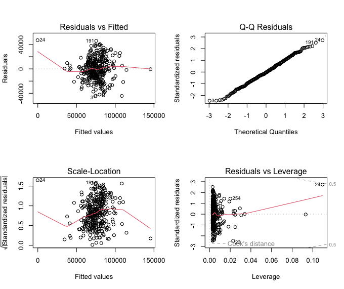

🗣️ DISCUSSION:

Is this a good fit? Why? Why not?

The residual plot suggests the relationship is not exactly linear. This model is not a good fit!

Part II - the `tidymodels` way (20 min)

👨🏻‍🏫 TEACHING MOMENT: Your class teacher will demonstrate how to get the same thing done using the tidymodels framework.

Task 3: Run a linear regression model with SalesVolume as the dependent variable and monthlyChangeHPI as the independent variable. Save the model as model2.

model2 <-
    linear_reg() %>%
    set_engine("lm") %>%
    fit(SalesVolume ~ monthlyChangeHPI, data = df_england)

Print the model coefficients in a tidy way:

model2 %>% tidy()

# A tibble: 2 × 5
  term             estimate std.error statistic   p.value
  <chr>               <dbl>     <dbl>     <dbl>     <dbl>
1 (Intercept)        69428.     1109.      62.6 1.16e-187
2 monthlyChangeHPI   12009.      944.      12.7 1.45e- 30

See the full model summary:

model2$fit %>% summary()

Call:
stats::lm(formula = SalesVolume ~ monthlyChangeHPI, data = data)

Residuals:
   Min     1Q Median     3Q    Max 
-44887 -11960   -548  12247  47019 

Coefficients:
                 Estimate Std. Error t value Pr(>|t|)    
(Intercept)       69427.6     1108.9   62.61   <2e-16 ***
monthlyChangeHPI  12008.9      943.6   12.73   <2e-16 ***
---
Signif. codes:  0 ‘***’ 0.001 ‘**’ 0.01 ‘*’ 0.05 ‘.’ 0.1 ‘ ’ 1

Residual standard error: 18300 on 337 degrees of freedom
  (323 observations deleted due to missingness)
Multiple R-squared:  0.3246,    Adjusted R-squared:  0.3226 
F-statistic:   162 on 1 and 337 DF,  p-value: < 2.2e-16

Overall statistics:

model2 %>% glance()

# A tibble: 1 × 12
  r.squared adj.r.squared  sigma statistic  p.value    df logLik   AIC   BIC      deviance df.residual  nobs
      <dbl>         <dbl>  <dbl>     <dbl>    <dbl> <dbl>  <dbl> <dbl> <dbl>         <dbl>       <int> <int>
1     0.325         0.323 18300.      162. 1.45e-30     1 -3807. 7620. 7632. 112860738556.         337   339

Task 4: Augument the model with the residuals and the fitted values and use the resulting data frame to plot the residuals against the fitted values.

model2 %>% augment(df_england)

# A tibble: 662 × 6
    .pred  .resid date       region  monthlyChangeHPI SalesVolume
    <dbl>   <dbl> <date>     <chr>              <dbl>       <dbl>
 1 80236.     NA  2023-06-01 England              0.9          NA
 2 68227.     NA  2023-05-01 England             -0.1          NA
 3 74231. -44887. 2023-04-01 England              0.4       29344
 4 57419. -16354. 2023-03-01 England             -1         41065
 5 63423. -23748. 2023-02-01 England             -0.5       39675
 6 59820. -18049. 2023-01-01 England             -0.8       41771
 7 61021.  -4138. 2022-12-01 England             -0.7       56883
 8 74231.  -8944. 2022-11-01 England              0.4       65287
 9 67026.  -2499. 2022-10-01 England             -0.2       64527
10 76633.  -9165. 2022-09-01 England              0.6       67468
# ℹ 652 more rows
# ℹ Use `print(n = ...)` to see more rows

Then use ggplot2 to plot the residuals against the fitted values:

ggplot(model2 %>% augment(df_england), aes(.pred, .resid)) + 
    geom_point()

You can further customise the plot:

plot_df <- model2 %>% augment(df_england)
g <- ggplot(plot_df, aes(x = .pred, y = .resid)) +
    geom_point(alpha=0.2, size=3, color="red", stroke=1) +
    geom_hline(yintercept = 0, linetype = "dashed") +
    labs(x = "Fitted values", y = "Residuals", title="Residuals vs Fitted") + 
    theme_bw() + 
    theme(axis.title.x = element_text(size = rel(1.2)), 
          axis.text.x = element_text(size = rel(1.2)),
          axis.title.y = element_text(size = rel(1.2)),
          axis.text.y = element_text(size = rel(1.2)),
          plot.title = element_text(size = rel(1.5), face = "bold"))
g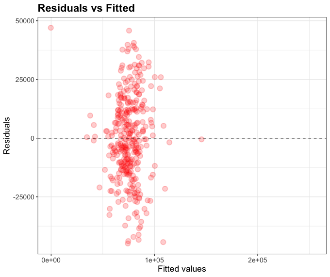

Part III - evaluating the model

STEP 01

Separate the data into training and testing sets. The training set must contain data up until Dec 2020. The testing set must contain data from Jan 2021 onwards.

The reasoning here is as follows:

I need to split my data into two separate data frames.
The questions specifies what it calls ‘training set’ as all the data up until Dec 2020.
Since we are subsetting the data by selecting rows, we can use the filter function to select the rows we need.
To make date comparisons, it is imperative that all date objects and columns are stored as proper date objects.
I have already properly modified the data type of the date column using lubridate. Therefore, I don’t need to modify anything else in that column.
However, I need to convert the string of text "2021-01-01" to a proper date object. I can use lubridate’s ymd function to convert a string to a date object.
Great, now I can use the filter function to select the rows I need.

df_england_train <- df_england %>% filter(date <   ymd("2021-01-01"))
df_england_test  <- df_england %>% filter(date >=  ymd("2021-01-01"))

Why do you need to convert date-related columns and objects to a date object using lubridate? The original data set has date in the format “DD/MM/YYYY” as a string. If you try to compare strings, you will get the wrong result because the comparison is done lexicographically (i.e. by alphabetical order).

For example, the following code will return TRUE, implying that 1 January 2021 happens before 1 December 2020:

"01/01/2021" < "01/12/2020"

[1] TRUE

STEP 02

Fit a linear regression model with tidymodels using just the training set. Call it model3. How does this model compare to the one you fitted in Part II?

How would you reason about this?

I need to fit a linear regression model using tidymodels. That is, copying the code from Part II (not with lm()).
I need to modify just the source of the data. Instead of using the entire data set, I need to use just the training set I created in STEP 01.

model3 <-
    linear_reg() %>%
    set_engine("lm") %>%
    fit(SalesVolume ~ monthlyChangeHPI, data = df_england_train)

In terms of comparison, if I tidy up the output of this new model, I will notice that it is quite similar to the one we fitted in Part II.

model3 %>% tidy()

# A tibble: 2 × 5
  term             estimate std.error statistic   p.value
  <chr>               <dbl>     <dbl>     <dbl>     <dbl>
1 (Intercept)        69260.     1161.      59.7 1.32e-171
2 monthlyChangeHPI   14041.     1107.      12.7 5.64e- 30

STEP 03

Calculate the Mean Absolute Error (MAE) for the training set. That is, on average, how far off is the model from the actual data?

How would you reason about this?

I don’t know what the MAE is. I need to look it up.
I go to the tidymodels website and search for “MAE” and “Mean Absolute Error”
The results didn’t exactly showed me how to calculate the MAE. I wonder if there is something in one of the packages that are part of tidymodels.
Eventually, you should find the yardstick package. You can read the documentation of the mae() function here.
From the documentation of the mae() function, I look at the examples and deduce that I need to compare the model predictions with the actual values used to fit it.
I can use the augment() function to get the predictions of the model on the training set. Then I can use the mae() function to calculate the MAE.

model3 %>% 
    augment(df_england_train) %>%
    mae(truth = SalesVolume, estimate = .pred)

# A tibble: 1 × 3
  .metric .estimator .estimate
  <chr>   <chr>          <dbl>
1 mae     standard      14213.

I am just printing out the value, but - alternatively - I can save it in a variable if I need to use it later:

mae_train <- 
    model3 %>% 
    augment(df_england_train) %>%
    mae(truth = SalesVolume, estimate = .pred)
mae_train

# A tibble: 1 × 3
  .metric .estimator .estimate
  <chr>   <chr>          <dbl>
1 mae     standard      14213.

The MAE is approximately 14213. That means on average, the model is off by 14213.

STEP 04

Calculate the Mean Absolute Error (MAE) for the testing set. That is, on average, how far off is the model from the actual data?

Here is when things start to get interesting. How would you reason about this?

I have already trained a model, model3 on two variables: SalesVolume and monthlyChangeHPI.
This means I can use the model to predict the SalesVolume for any given value of monthlyChangeHPI, on any data set – it does not have to be the same data I used to train the model.
Therefore, I can use the augment() function to get the predictions of the model on the testing set. Then I can use the mae() function to calculate the MAE, just the same way I did before.

model3 %>% 
    augment(df_england_test) %>%
    mae(truth = SalesVolume, estimate = .pred)

# A tibble: 1 × 3
  .metric .estimator .estimate
  <chr>   <chr>          <dbl>
1 mae     standard      20323.

OH WOW! This is a much higher error than the one we got for the training set. The model is wrong on average almost twice as much as it was on the training set. This can happen for many reasons: it could be that the model is so attuned to the training set that it is not able to generalise to the testing set, or it could mean that something changed in the dynamics that produced this data, and the model – fitted on older data – is not able to capture it. Which one do you think it is?

💡 A common source of confusion in this question was that many people assumed that we would have to train a new model. That is not the case, and this is the beauty of modelling. Once you have a model, you can use it to predict the outcome on any data set, as long as the data set has the same variables as the ones you used to train the model. (We will explore more of the implications and limitations of thinking this way in the future, in this course)

STEP 05

Now, add a second independent variable, call it monthlyChangeHPI_lag1, which is essentially a lagged variable of the monthlyChangeHPI variable you already have. Build a new model, call it model4, and compare it to model3. Which one is better?

Let’s start by modifying our original England data set/data frame to add the new second independent variable that we’re creating, i.e the lagged variable monthlyChangeHPI_lag1

df_england <- 
    df_england %>%
    arrange(date) %>% # Sort in ascending order so we can use lag later
    mutate(monthlyChangeHPI_lag1 = lag(monthlyChangeHPI, 1)) %>%
    drop_na() %>%
    arrange(desc(date))

Then, as we did before, we split our dataset into training and test set:

df_england_train <- df_england %>% filter(date <   ymd("2021-01-01"))
df_england_test  <- df_england %>% filter(date >=  ymd("2021-01-01"))

We then build our new linear regression model model4 that takes, as before, SalesVolume as dependent variable but, this time, two independent variables instead of just one, monthlyChangeHPI and the newly-created monthlyChangeHPI_lag1:

model4 <-
  linear_reg() %>%
  set_engine("lm") %>%
  fit(SalesVolume ~ monthlyChangeHPI + monthlyChangeHPI_lag1, data = df_england_train)

If we tidy the output of this new model, here is what we get:

model4 %>% tidy()

# A tibble: 3 × 5
  term                  estimate std.error statistic   p.value
  <chr>                    <dbl>     <dbl>     <dbl>     <dbl>
1 (Intercept)             67704.     1122.     60.3  2.64e-172
2 monthlyChangeHPI         8477.     1343.      6.31 9.62e- 10
3 monthlyChangeHPI_lag1    8710.     1342.      6.49 3.46e- 10

Notice that both independent variables used in the regression, i.e monthlyChangeHPI and monthlyChangeHPI_lag1 contribute relatively equally to the model…

What about the MAE for this model?

model4 %>% 
  augment(df_england_train) %>%
  mae(truth = SalesVolume, estimate = .pred)

# A tibble: 1 × 3
  .metric .estimator .estimate
  <chr>   <chr>          <dbl>
1 mae     standard      13331.

For the training set, the MAE for model4 is slightly lower than for model3.

model4 %>% 
  augment(df_england_test) %>%
  mae(truth = SalesVolume, estimate = .pred)

# A tibble: 1 × 3
  .metric .estimator .estimate
  <chr>   <chr>          <dbl>
1 mae     standard      17510.

When it comes to test set too, the performance of model4 is better than that of model3.

It looks as if model4 fits the data better than model3!

STEP 06

Now create a df_scotland with the same variables as df, but only for Scotland (no need to separate into training and testing sets).

I can use the same code I used to create df_england in the beginning of this lab, but I need to change the filter condition to select only Scotland:

df_scotland <-
    uk_hpi %>%
    select(all_of(selected_cols)) %>%
    rename(date = Date, region = RegionName, monthlyChangeHPI = `1m%Change`) %>%
    filter(region == "Scotland") %>%
    drop_na(monthlyChangeHPI) %>% 
    mutate(date = lubridate::dmy(date)) %>% 
    arrange(date) %>%
    mutate(monthlyChangeHPI_lag1 = lag(monthlyChangeHPI, 1)) %>%
    drop_na() %>%
    arrange(desc(date))

Checking that it is correct:

df_scotland %>% head(8)

# A tibble: 8 × 5
  date       region   monthlyChangeHPI SalesVolume monthlyChangeHPI_lag1
  <date>     <chr>               <dbl>       <dbl>                 <dbl>
1 2023-04-01 Scotland              1.4        6902                   1  
2 2023-03-01 Scotland              1          8026                  -1.4
3 2023-02-01 Scotland             -1.4        5413                  -0.4
4 2023-01-01 Scotland             -0.4        5866                  -3.5
5 2022-12-01 Scotland             -3.5        7862                   0.1
6 2022-11-01 Scotland              0.1        9047                   0  
7 2022-10-01 Scotland              0          9170                  -0.3
8 2022-09-01 Scotland             -0.3       10097                   0.1

Further sanity check:

df_scotland$region %>% unique() # Retrieve all unique values in the `region` column

[1] "Scotland"

STEP 07

How well can model3 and model4 predict monthly changes in house prices in Scotland?

Now that you have realised that model3 can be used in any dataset, you can use it to predict the monthly changes in house prices in Scotland the same way you did for the England test set. We can also calculate the MAE so we can compare it with the MAE we calculated for the England test set.

model3 %>% 
    augment(df_scotland) %>%
    mae(truth = SalesVolume, estimate = .pred)

# A tibble: 1 × 3
  .metric .estimator .estimate
  <chr>   <chr>          <dbl>
1 mae     standard      66164.

The error is also much higher, on average, than the one we got for the England training set. This is not surprising, since the model was trained on England data, and Scotland is a different country with different dynamics.

(Extra) Out of curiosity, we could see if the MAE changes over time. I could group the data by year and calculate the MAE for each year:

model3 %>%
    augment(df_scotland) %>%
    group_by(year = lubridate::year(date)) %>%
    mae(SalesVolume, .pred) # MAE is already a summary statistics, so I don't need to use summarise()

While I am at it, I can plot it:

plot_df <- 
    model3 %>%
    augment(df_scotland) %>%
    group_by(year = lubridate::year(date)) %>%
    mae(SalesVolume, .pred)

g <- 
    (
        ggplot(plot_df, aes(x=year, y=.estimate, color=.metric))
            + geom_line()
            + geom_point()
            + ylim(c(0, NA)) # Ensure the Y axis starts at zero. NA means "whatever the maximum value is"
            + labs(x = "Year", y = "MAE", title="MAE over time")
    )
g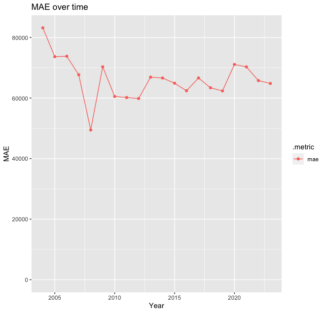

Interestingly, the worst predictions were for 2004, not during the pandemic. This is indicative that the dynamics in Scotland changed around that time, and the model is not able to capture it as it was trained on data from a different country!

Let’s do the same for model4. Is model4 a better fit for Scotland than model3 was?

model4 %>% 
  augment(df_scotland) %>%
  mae(truth = SalesVolume, estimate = .pred)

# A tibble: 1 × 3
  .metric .estimator .estimate
  <chr>   <chr>          <dbl>
1 mae     standard      66065.

The error is still much higher, on average, than for this model the one we got for the England training set. The same conclusions that applied for model3 apply here as well!

Let’s, as before, plot MAE over time:

plot_df <- 
  model4 %>%
  augment(df_scotland) %>%
  group_by(year = lubridate::year(date)) %>%
  mae(SalesVolume, .pred)

g <- 
  (
    ggplot(plot_df, aes(x=year, y=.estimate, color=.metric))
    + geom_line()
    + geom_point()
    + ylim(c(0, NA)) # Ensure the Y axis starts at zero. NA means "whatever the maximum value is"
    + labs(x = "Year", y = "MAE", title="MAE over time")
  )
g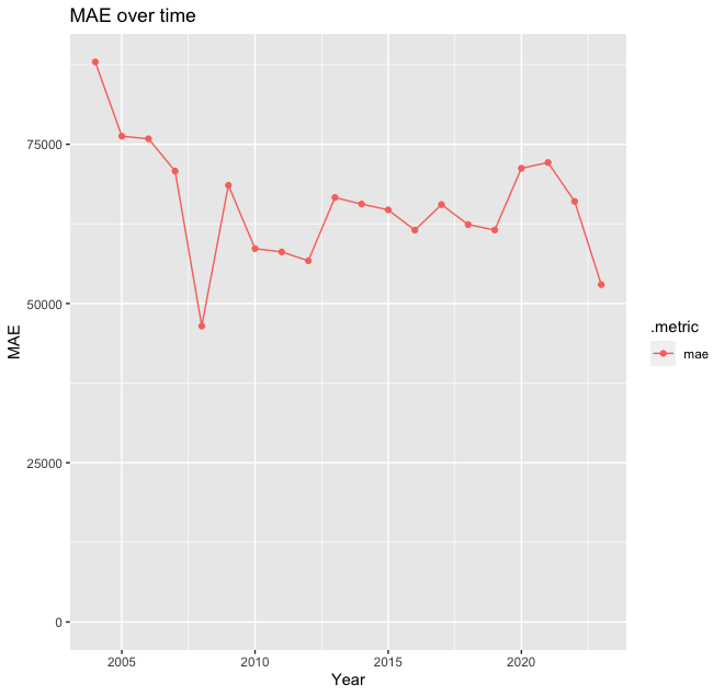

MAE is highest, as before, in 2004: this is the second model to suggest that the dynamics of the housing market in Scotland experienced some changes around that time, and the model is not able to capture it as it was trained on data from a different country! Some deeper investigations are needed here!

⚙️ Setup

📋 Lab Tasks

Part I - the lm command (25 min)

Part II - the tidymodels way (20 min)

Part III - evaluating the model

Part I - the `lm` command (25 min)

Part II - the `tidymodels` way (20 min)