DS202A Week 02 - Source Code - Part I

Author

Published

10 Oct 2023

This .qmd is an expanded version of what I taught in the Week 02 lecture.

Click on the button below to download the source files that were used to create this page:

(this is a zip file because there are images in it)

Files, folders, and paths in RStudio

Before you even start coding, it is important to understand RStudio panes a bit more deeply. If you have not spent a lot of time creating your own R Scripts, you might likely have some knowledge gaps about where your files are stored, how to create folders, and how to set your working directory.

Where are you?

(If you are taking or have already taken DS105, you likely have a deep understanding of this topic. You can probably skip this section.)

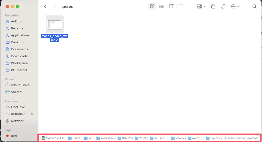
Your computer is full of different folders (also called ‘directories’) organised hierarchically. For example, on macOS’s Finder, this is the path that leads to an image I created deep inside my DS202 folder:

(On Windows, the File Explorer looks very similar but is typically represented on the left-hand side of the screen.)

Notice how many different steps I had to take to get to this image. I had to go through my Users folder, then my jon folder, then my DS202 folder, eventually getting to the mac_os_finder_example.png file. This is called a full path and can also be represented as a string of text:

/Users/jon/Workspace/DS202/2023/autumn-term/weeks/week02/figures/macos_finder_example.png

We call this path full because we started from the very top of the hierarchy (the Users folder) and went all the way down to the file we wanted to access. If I was inside the DS202 folder and I wanted to represent the path to the image above, I could use a relative path:

./2023/autumn-term/weeks/week02/figures/macos_finder_example.png

where the dot (.) represents the current folder I am in.

There is one special folder that you might encounter which is represented by the tilde (~). This is your home folder. It is the place where the typical folders you use are: Documents, Downloads, Desktop, etc.

In the example above, ~ is merely a replacement for /Users/jon. Therefore, I could have also used the following relative path to refer to the exact same file:

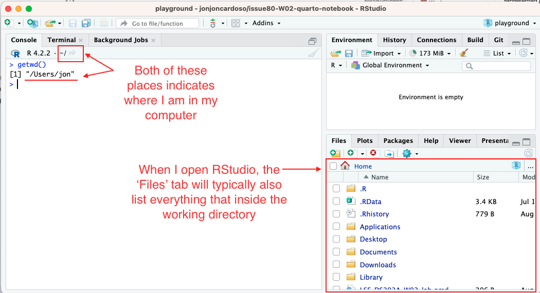
~/Workspace/DS202/2023/autumn-term/weeks/week02/figures/macos_finder_example.png

What does this have to do with RStudio?

RStudio (and also VSCode) has this concept of a working directory. It represents where you are in your computer’s hierarchy. You can check where you are by running the following command in the R Console:

getwd()

By default, when you open RStudio after installing it for the very first time, you are typically automatically placed in your home folder. If that is your case, you will see something like this:

If you don’t like where you are (or if you are not sure where you are), you can set your working directory to a different location. For example, if you want your working directory to be your home folder, you can run the following command:

setwd("~")

⚠️ Now here is the danger: the ‘Files’ tab is not synced with the working directory. You can change your working directory to your home folder, but the ‘Files’ tab will still show you the contents of the folder you were in before. This can be very confusing, so be careful!

☢️ It gets worse: When you create a new file, say a .qmd file, RStudio does not save it anywhere until you click ‘Save’ (or Ctrl+S). When you save the file, you need to be extra hyper-aware of where you are saving it. If you are not, you might end up saving it in a completely different folder than you intended to, leading to:

☣️ The worst-case scenario: This is when you are somewhere in your R Console, somewhere else in the Files tab and your notebook is saved in a completely different folder. This is a recipe for disaster.

Best practices

Here are some best practices to avoid the worst-case scenario:

Dedicate one specific folder for all the files you will be creating in this course. The simplest way to ensure things are synchronised is by creating a Project within RStudio (Go to the menu at the top of the app then click on File -> New Project -> New Directory -> Project Type: New Project -> then choose the path).

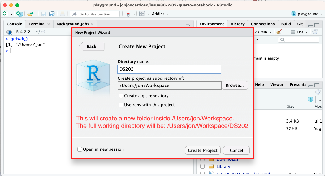
Use the same project throughout this course. No need to create new projects. If you need to organise your files, create folders within your project.
If you use the Files tab to see what is inside your project, create the habit of going back to where your working directory is.
If you use projects as I recommend above, don’t change the working directory any more, nor use setwd() at all. You no longer need to tweak that - it will only confuse you.
If you want to read a file that is inside a sub-folder of your project, use a relative path. For example, if you want to read a file called my_file.csv that is inside a folder called data, you can use the following command:
```
readr::read_csv("./data/my_file.csv")
```
you can even omit the . in these cases and just use:
```
readr::read_csv("data/my_file.csv")
```

Quarto Markdown

If you are reading this from Moodle or the public course website, all you see is a beautiful HTML page - just like any other page you encounter on the Web. But what you see now is not what I see when I am editing this file. To get the same experience, go to the top of this page and click on the Download button to get a copy of this file plus the figures used in its original form, as a .qmd file, copy it to your working directory inside RStudio and then open it.

You will notice that when I use #, this gets converted to a huge title when seen as a webpage, like the Quarto Markdown title at the start of this section. Notice how, on the web page, the #’s that demarcate the preceding sections are gone (You see Quarto Markdown, not #Quarto Markdown). This is possible because of something called the Markdown language.

Click on this link to read more about how to use Markdown.

You will see for example that I can create sub-titles by appending more #s, like this:

# Quarto Markdown

## Sub-title

### Sub-sub-title

And that I can make this text bold by surrounding it with two asterisks.

If I want to use R code to illustrate a point, I can use three backticks + the character r to create a code block, that is: ```r. For example, look at the code below:

readr::read_csv("data/my_file.csv")

If you are seeing this in your Quarto markdown file, you will see the preceding ```r followed by the code probably highlighted in different colours, then the closing backticks, ```. When you see this markdown rendered as an HTML webpage, however, you won’t see any of the backticks, you will just see some R code coloured nicely.

The code block above only shows code, it does not run any code. If you need code that runs, you have to use the ```{r} syntax. This code block, also called a chunk is a bit more complex and you can customise it in many ways.

Here is an example:

my_variable <- "This is a string variable in R"

# When I render this file to an HTML, you will see the result of the print below
print(my_variable)

[1] "This is a string variable in R"

Give it a go: click ‘Render’ at the top of RStudio and see what happens. You will see the result of the print() function below the code block.

⚠️ IMPORTANT: if your R code has errors, you won’t be able to render your .qmd file as an HTML webpage. You will have to fix the errors first! Also, the .qmd always runs from top to bottom and it ignores any code that is not part of it. So, if you typed something in R Console that you want to use in your .qmd, you have to copy and paste it into your .qmd file.

Mix of tips

Notice how I customised my name, the title and date of this Quarto Markdown by adjusting the very first lines of this file:

---
title: "DS202A Week 02 - Source Code"
author: "[Dr. Jon Cardoso-Silva](https://jonjoncardoso.github.io)"
date: "2023-10-10"
...

I also recommend that you add the following two lines so that your .qmd file produces just one single HTML file:
```
---
...
format: html
self-contained: true
---
```