
✅ LSE DS202A 2025: Week 03 - Lab Solutions
This solution file follows the format of the .qmd notebook you had to fill in during the lab session.
Downloading the student solutions
Click on the below button to download the student notebook.
Loading libraries and functions
library("colino")
library("ggsci") # For pretty colour schemes
library("MASS") # For simulating data
library("scales") # For number formatting in ggplot2
library("tidymodels") # For train / test splits
library("tidyverse") # For data wrangling / visualisation

# Let's use some of the theme functions we created in lab 2

theme_histogram <- function() {
  theme_minimal() +
    theme(
      panel.grid.minor = element_blank(),
      panel.grid.major.x = element_blank()
    )
}

theme_boxplot <- function() {
  theme_minimal() +
    theme(
      panel.grid.minor = element_blank(),
      panel.grid.major.x = element_blank(),
      legend.position = "none"
    )
}

theme_bar <- function() {
  theme_minimal() +
    theme(
      panel.grid.minor = element_blank(),
      panel.grid.major.y = element_blank()
    )
}

theme_scatter <- function() {
  theme_minimal() +
    theme(panel.grid.minor = element_blank(), legend.position = "bottom")
}
Before we do anything more
Please create a data folder called data to store all the different data sets in this course.
Student Performance
students <- read_csv("data/students-data-cleaned.csv")We start our machine learning journey with a student performance dataset (students), which contains information on students from two Portuguese schools. We have cleaned the data to only include statistically significant predictors. The columns include:
final_grade- final grade from 0 to 20 (the outcome) •
school- student’s school (binary: ‘GP’ - Gabriel Pereira or ‘MS’ - Mousinho da Silveira)sex- student’s sex (binary: ‘F’ - female or ‘M’ - male) -age- student’s age (numeric: from 15 to 22)address- student’s home address type (binary: ‘U’ - urban or ‘R’ - rural)famsize- family size (binary: ‘LE3’ - less or equal to 3 or ‘GT3’ - greater than 3)pstatus- parent’s cohabitation status (binary: ‘T’ - living together or ‘A’ - apart)medu- mother’s education (numeric: 0 - none, 1 - primary education (4th grade), 2 - 5th to 9th grade, 3 - secondary education or 4 - higher education)fedu- father’s education (numeric: 0 - none, 1 - primary education (4th grade), 2 - 5th to 9th grade, 3 - secondary education or 4 - higher education)mjob- mother’s job (nominal: ‘teacher’, ‘health’ care related, civil ‘services’ (e.g. administrative or police), ‘at_home’ or ‘other’)fjob- father’s job (nominal: ‘teacher’, ‘health’ care related, civil ‘services’ (e.g. administrative or police), ‘at_home’ or ‘other’)reason- reason to choose this school (nominal: close to ‘home’, school ‘reputation’, ‘course’ preference or ‘other’guardian- student’s guardian (nominal: ‘mother’, ‘father’ or ‘other’)traveltime- home to school travel time (numeric: 1 - <15 min., 2 - 15 to 30 min., 3 - 30 min. to 1 hour, or 4 - >1 hour)studytime- weekly study time (numeric: 1 - <2 hours, 2 - 2 to 5 hours, 3 - 5 to 10 hours, or 4 - >10 hours)failures- number of past class failures (numeric: n if 1<=n<3, else 4)schoolsup- extra educational support (binary: yes or no)famsup- family educational support (binary: yes or no)paid- extra paid classes within the course subject (Math or Portuguese) (binary: yes or no)activities- extra-curricular activities (binary: yes or no)nursery- attended nursery school (binary: yes or no)higher- wants to take higher education (binary: yes or no)internet- Internet access at home (binary: yes or no)romantic- with a romantic relationship (binary: yes or no)famrel- quality of family relationships (numeric: from 1 - very bad to 5 - excellent)freetime- free time after school (numeric: from 1 - very low to 5 - very high)goout- going out with friends (numeric: from 1 - very low to 5 - very high)dalc- workday alcohol consumption (numeric: from 1 - very low to 5 - very high)walc- weekend alcohol consumption (numeric: from 1 - very low to 5 - very high)health- current health status (numeric: from 1 - very bad to 5 - very good)absences- number of school absences (numeric: from 0 to 93)
Understanding student performance: some exploratory data analysis (EDA) (10 minutes)
Now it’s your turn to explore the students dataset! Use this time to create visualizations and discover patterns in the data that might help explain what drives student success.
Some ideas to get you started:
- How are final grades distributed? Are they normally distributed or skewed?
- Do students who want higher education perform better than those who don’t?
- Is there a relationship between study time and final grades?
- How does past academic failure affect current performance?
- Are there differences in performance between the two schools?
- Does going out with friends impact academic performance?
- What’s the relationship between health status and grades?
- Do students receiving extra educational support perform differently?
Challenge yourself:
- Can you find any surprising relationships in the data?
- What patterns emerge when you look at combinations of variables?
- Are there any outliers or interesting edge cases?
Share your most interesting findings on Slack! We’d love to see what patterns you discover and which visualizations tell the most compelling stories about student performance.
# Your EDA code here!
# Try different plot types: histograms, boxplots, scatter plots, bar charts
# Example starter code:

students |>
  ggplot(aes(x = final_grade)) +
  geom_histogram()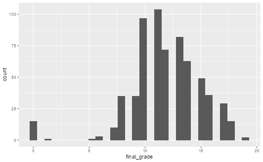
Understanding student performance: the hypothesis-testing approach (5 minutes)
Why do some students perform better than others? This is one question that a quantitative social scientist might answer by exploring the magnitude and precision of a series of variables. Suppose we hypothesised that students who want to pursue higher education have better academic performance. We can estimate a linear regression model by using final_grade as the dependent variable and higher as the independent variable.
To run a linear regression, we can use the lm function, which requires two things:
- A model formula (a.k.a. equation)
- The data used to estimate the model
Let’s do this now. We can call the summary function to get information on the coefficient estimate for higher.
lm(final_grade ~ higher, data = students) |>
  summary()

Call:
lm(formula = final_grade ~ higher, data = students)

Residuals:
     Min       1Q   Median       3Q      Max
-12.2759  -1.2759  -0.2759   1.7241   6.7241

Coefficients:
            Estimate Std. Error t value Pr(>|t|)
(Intercept)   8.7971     0.3671  23.962   <2e-16 ***
higheryes     3.4788     0.3883   8.958   <2e-16 ***
---
Signif. codes:  0 ‘***’ 0.001 ‘**’ 0.01 ‘*’ 0.05 ‘.’ 0.1 ‘ ’ 1

Residual standard error: 3.05 on 647 degrees of freedom
Multiple R-squared:  0.1103,    Adjusted R-squared:  0.109
F-statistic: 80.24 on 1 and 647 DF,  p-value: < 2.2e-16
We see that students who want to pursue higher education have a positive and statistically significant (p < 0.001) increase in final grades of about 3.5 points.
👉 NOTE: The process of hypothesis testing is obviously more involved when using observational data than is portrayed by this simple example. Control variables will almost always be incorporated and, increasingly, identification strategies will be used to uncover causal effects. The end result, however, will involve as rigorous an attempt at falsifying a hypothesis as can be provided with the data.
For an example of how multivariate regression is used, we can run the following code.
lm(final_grade ~ ., data = students) |>
  summary()

Call:
lm(formula = final_grade ~ ., data = students)

Residuals:
     Min       1Q   Median       3Q      Max
-11.7275  -1.3732   0.1009   1.5526   7.3862

Coefficients:
                    Estimate Std. Error t value Pr(>|t|)
(Intercept)          7.30785    2.54277   2.874 0.004202 **
schoolMS            -1.11221    0.27336  -4.069 5.39e-05 ***
sexM                -0.72456    0.24955  -2.904 0.003831 **
age                  0.20145    0.10269   1.962 0.050275 .
addressU             0.40454    0.26203   1.544 0.123168
famsizeLE3           0.29420    0.24433   1.204 0.229045
pstatusT             0.28615    0.34907   0.820 0.412702
meduPrimary          0.25719    1.15015   0.224 0.823137
medu5th-9th          0.02378    1.15816   0.021 0.983624
meduSecondary        0.17393    1.17222   0.148 0.882098
meduHigher           0.36932    1.20668   0.306 0.759670
feduPrimary         -1.16578    1.07170  -1.088 0.277140
fedu5th-9th         -0.70044    1.08083  -0.648 0.517205
feduSecondary       -0.72657    1.10120  -0.660 0.509643
feduHigher          -0.35673    1.13248  -0.315 0.752874
mjobhealth           0.70046    0.54668   1.281 0.200602
mjobother            0.02909    0.30317   0.096 0.923583
mjobservices         0.48291    0.37275   1.296 0.195652
mjobteacher          0.15798    0.52398   0.301 0.763147
fjobhealth          -0.65551    0.75511  -0.868 0.385698
fjobother            0.01680    0.45963   0.037 0.970861
fjobservices        -0.42321    0.48310  -0.876 0.381381
fjobteacher          0.64758    0.69123   0.937 0.349223
reasonhome          -0.11480    0.28321  -0.405 0.685363
reasonother         -0.57702    0.36240  -1.592 0.111880
reasonreputation     0.05013    0.29638   0.169 0.865753
guardianmother      -0.35945    0.26535  -1.355 0.176073
guardianother        0.24572    0.53496   0.459 0.646173
traveltime15-30min   0.09210    0.24772   0.372 0.710193
traveltime30min-1hr  0.60224    0.42640   1.412 0.158380
traveltime>1hr      -0.51974    0.72346  -0.718 0.472792
studytime2-5hrs      0.32059    0.26629   1.204 0.229117
studytime5-10hrs     0.92405    0.36509   2.531 0.011638 *
studytime>10hrs      0.97285    0.51866   1.876 0.061198 .
failures1           -2.64004    0.37785  -6.987 7.74e-12 ***
failures2           -3.04327    0.73865  -4.120 4.34e-05 ***
failures3           -2.98888    0.76691  -3.897 0.000109 ***
schoolsupyes        -1.14529    0.36452  -3.142 0.001764 **
famsupyes           -0.12318    0.22828  -0.540 0.589683
paidyes             -0.26061    0.45938  -0.567 0.570725
activitiesyes        0.18262    0.22327   0.818 0.413741
nurseryyes          -0.09086    0.27264  -0.333 0.739053
higheryes            1.55928    0.38493   4.051 5.80e-05 ***
internetyes          0.29038    0.27702   1.048 0.294973
romanticyes         -0.35903    0.23038  -1.558 0.119688
famrelBad            0.27599    0.78502   0.352 0.725286
famrelAverage        0.51891    0.66642   0.779 0.436504
famrelGood           1.06771    0.62457   1.710 0.087892 .
famrelExcellent      0.64974    0.63744   1.019 0.308493
freetimeLow          0.45627    0.48805   0.935 0.350242
freetimeAverage     -0.20749    0.44806  -0.463 0.643484
freetimeHigh        -0.06067    0.47752  -0.127 0.898943
freetimeVeryHigh    -0.16014    0.55132  -0.290 0.771565
gooutLow             1.51599    0.45708   3.317 0.000968 ***
gooutAverage         1.08580    0.44860   2.420 0.015809 *
gooutHigh            0.92551    0.47878   1.933 0.053714 .
gooutVeryHigh        0.48026    0.50828   0.945 0.345121
dalcLow             -0.34567    0.32278  -1.071 0.284640
dalcAverage          0.29935    0.51598   0.580 0.562035
dalcHigh            -2.18846    0.72651  -3.012 0.002706 **
dalcVeryHigh        -0.46026    0.84155  -0.547 0.584646
walcLow             -0.11154    0.29771  -0.375 0.708055
walcAverage         -0.26810    0.34007  -0.788 0.430801
walcHigh            -0.37326    0.42431  -0.880 0.379389
walcVeryHigh         0.11392    0.63865   0.178 0.858492
healthBad           -0.27317    0.42497  -0.643 0.520605
healthAverage       -0.76200    0.38083  -2.001 0.045870 *
healthGood          -0.32390    0.39305  -0.824 0.410239
healthVeryGood      -0.97409    0.34813  -2.798 0.005311 **
absences            -0.02242    0.02478  -0.905 0.365952
---
Signif. codes:  0 ‘***’ 0.001 ‘**’ 0.01 ‘*’ 0.05 ‘.’ 0.1 ‘ ’ 1

Residual standard error: 2.593 on 579 degrees of freedom
Multiple R-squared:  0.4244,    Adjusted R-squared:  0.3558
F-statistic: 6.188 on 69 and 579 DF,  p-value: < 2.2e-16
The . placeholder indicates that we want to use all other variables in the data set. We can see that the coefficient estimate for higher approximately halves in size yet remains positive and highly significant (p < 0.001), suggesting this relationship holds even when controlling for other factors like study time, past failures, and demographic characteristics.
👉 NOTE: p-values are useful to machine learning scientists as they indicate which variables may yield a significant increase in model performance. However, p-hacking where researchers manipulate data to find results that support their hypothesis make it hard to tell whether or not a relationship held up after honest attempts at falsification. This can range from using a specific modelling approach that produces statistically significant (while failing to report others that do not) findings to outright manipulation of the data. For a recent egregious case of the latter, we recommend the Data Falsificada series.
Predicting student grades: the machine learning approach (30 minutes)
Machine learning scientists take a different approach. Our aim, in this context, is to build a model that can be used to accurately predict how happy a person is using a mixture of features and, for some models, hyperparameters (which we will address in Lab 5).
Thus, rather than attempting to falsify the effects of causes, we are more concerned about the fit of the model in the aggregate when applied to unforeseen data.
To achieve this, we do the following:
- Split the data into training and test sets
- Build a model using the training set
- Evaluate the model on the test set
Let’s look at each of these in turn.
Split the data into training and test sets
It is worth considering what a training and test set is and why we might split the data this way.
A training set is data that we use to build (or “train”) a model. In the case of multivariate linear regression, we are using the training data to estimate a series of coefficients. Here is a made-up multivariate linear model with three coefficients derived from (non-existent) data to illustrate things.
sim_model_preds <- function(x1, x2, x3) {
  y <- 1.1 * x1 + 2.2 * x2 + 3.3 * x3
  y
}
A test set is data that the model has not yet seen. We then apply the model to this data set and use an evaluation metric to find out how accurate our predictions are. For example, suppose we had a new observation where x1 = 10, x2 = 20 and x3 = 30 and y = 150. We can use the above model to develop a prediction.
sim_model_preds(10, 20, 30)

[1] 154
We get a prediction of 154 points!
We can also calculate the amount of error we make by calculating residuals (actual value - predicted value).
150 - sim_model_preds(10, 20, 30)

[1] -4
We can see that our model is 4 points off the real answer!
Why do we evaluate our models using different data? Because, as stated earlier, machine learning scientists care about the applicability of a model to unforeseen data. If we were to evaluate the model using the training data, we obviously cannot do this to begin with. Furthermore, we cannot ascertain whether the model we have built can generalise to other data sets or if the model has simply learned the idiosyncrasies of the data it was used to train on. We will discuss the concept of overfitting throughout this course.
We can use the rsample package in the tidymodels ecosystem to split the data into training and test sets.
# Set a seed for reproducibility

set.seed(123)

# Split the data with 75% being used to train the model

students_split <- initial_split(students, prop = 0.75)

# Create tibbles of the training and test set

students_train <- training(students_split)
students_test <- testing(students_split)
👉 NOTE: Our data are purely cross-sectional, so we can use this approach. However, when working with more complex data structures (e.g. time series cross sectional), different approaches to splitting the data will need to be used.
Build a model using the training set
This is remarkably simple. We will use almost exactly the same code we used to build a multivariate linear model, but with one exception. Instead of using the whole of the data, we will only use students_train. We will also only create a model object (mv_model, short for multivariate model).
mv_model <- lm(final_grade ~ ., data = students_train)Evaluate the model using the test set
Now that we have trained a model, we can then evaluate its performance on the test set. We will look at two evaluation metrics:
- R-squared: the proportion of variance in the outcome explained by the model.
- Root mean squared error (RMSE): the amount of error a typical observation parameterised as the units used in the initial measurement.
reg_metrics <- metric_set(rsq, rmse)

mv_model |>
  augment(new_data = students_test) |>
  reg_metrics(truth = final_grade, estimate = .fitted)

# A tibble: 2 × 3
  .metric .estimator .estimate
  <chr>   <chr>          <dbl>
1 rsq     standard       0.468
2 rmse    standard       2.32
🗣️ CLASSROOM DISCUSSION:
How can we interpret these results?
We find that the model explains ~ 47% of the test set variance in final grades. We also find that our model predictions are off by ~ 2.3 points on the 0-20 grade scale.
Graphically exploring where we make errors
We are going to build some residual scatter plots which look at the relationship between the values fitted by the model for each observation and the residuals (actual - predicted values). Before we do this for our data, let’s take a look at an example where there is a near perfect relationship between two variables. As this very rarely exists in the social world, we will rely upon simulated data.
We adapted this code from here.
# Set a seed for reproducibility

set.seed(123)

# Create the variance covariance matrix

sigma <- rbind(c(1, 0.99), c(0.99, 1))

# Create the mean vector

mu <- c(10, 5)

# Generate a multivariate normal distribution using 1,000 samples

sim_data <-
  mvrnorm(n = 1000, mu = mu, Sigma = sigma) |>
  as.data.frame() |>
  as_tibble()
Plot the correlation
# Plot the correlation

ggplot(sim_data, aes(V1, V2)) +
  geom_point() +
  theme_scatter() +
  labs(x = "Variable 1", y = "Variable 2")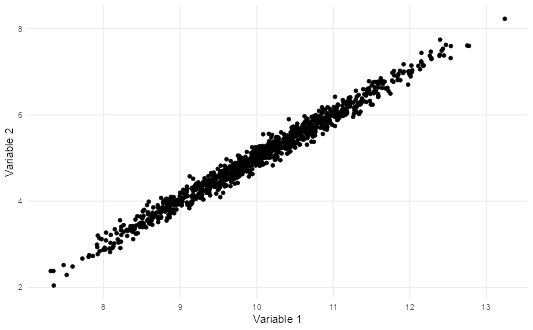
Residual plots
# Build a linear model and plot the fitted versus residual values

lm(V2 ~ V1, data = sim_data) |>
  augment() |>
  ggplot(aes(.fitted, .resid)) +
  geom_hline(yintercept = 0, linetype = "dashed") +
  geom_point() +
  theme_scatter() +
  labs(x = "Fitted values", y = "Residuals")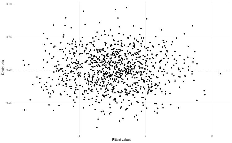
Now let’s run this code for our model.
mv_model |>
  augment(new_data = students_test) |>
  ggplot(aes(.fitted, .resid)) +
  geom_hline(yintercept = 0, linetype = "dashed") +
  geom_point() +
  theme_scatter() +
  labs(x = "Fitted values", y = "Residuals")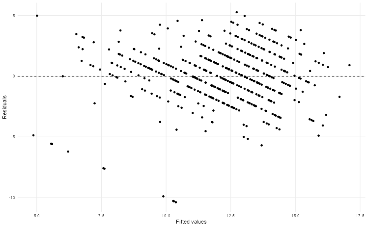
🎯 ACTION POINTS why does the graph of the simulated data illustrate a more well-fitting model when compared to our actual data?
The spread of our values in the actual data is relatively large. This suggests there may be non-linear relationships or missing variables that could improve our model.
Challenge: Experiment with Filter Methods (30 minutes)
🎯 YOUR CHALLENGE: Experiment with different filter methods for automatic feature selection using the colino package!
Your Mission
You started with this code that selects categorical features using ANOVA:
library("colino")

recipe(final_grade ~ ., data = students_train) |>
  step_select_aov(all_nominal(), -all_outcomes(), outcome = "final_grade", top_p = 5) |>
  prep() |>
  bake(new_data = NULL) |>
  glimpse()

Rows: 486
Columns: 8
$ school      <fct> GP, MS, GP, MS, GP, GP, GP, GP, GP, GP, GP, MS…
$ sex         <fct> F, F, M, M, M, M, F, F, F, M, F, F, F, F, F, F…
$ age         <int> 20, 15, 17, 17, 16, 16, 17, 17, 17, 15, 17, 18…
$ medu        <fct> Primary, Primary, Primary, Higher, Higher, Sec…
$ studytime   <fct> 5-10hrs, 2-5hrs, 2-5hrs, 5-10hrs, 2-5hrs, <2hr…
$ failures    <fct> 0, 0, 0, 0, 0, 0, 0, 0, 0, 0, 0, 0, 0, 0, 0, 0…
$ absences    <int> 8, 0, 0, 0, 4, 6, 2, 6, 0, 0, 0, 4, 0, 2, 0, 2…
$ final_grade <int> 15, 14, 8, 16, 11, 15, 12, 11, 16, 13, 10, 10,…
Explanation
The code above defines a data preprocessing recipe using the recipes package (part of the tidymodels framework) and applies ANOVA-based feature selection from the colino package.
ANOVA (Analysis of Variance) is a statistical method used to test whether there are significant differences between the means of a numeric outcome variable across different categories of a predictor variable. In this context, step_select_aov() evaluates each categorical predictor in relation to the target variable final_grade and computes an F-statistic for each. Variables with stronger relationships (i.e., higher F-statistics or lower p-values) are considered more relevant for predicting the outcome.
By setting top_p = 5, the recipe keeps the five most statistically significant nominal predictors, based on their ANOVA test results. In addition to these, any continuous or numeric predictors in the original dataset (such as age and absences) are retained automatically, since they are not part of the ANOVA selection step.
After applying the recipe (prep() + bake()), the resulting dataset contains:
- 486 rows — the same number of training observations as before.
- 8 columns — consisting of 7 predictors (
school,sex,age,medu,studytime,failures,absences) and the target variablefinal_grade.
This feature selection step helps simplify the model by focusing on the most informative predictors, potentially improving interpretability and reducing overfitting. The final dataset is now ready for subsequent modeling steps such as fitting a regression or classification model.
Now explore what other filter methods are available!
🔍 Your Resource
Read this page: https://tidymodels.aml4td.org/chapters/feature-selection.html#sec-automatic-selection
Look for different step_select_* functions and try them out!
🧪 Experiments to Try
Experiment 1: Different Selection Functions
Find and try 2-3 different step_select_* functions from the documentation:
🎯 What to Report
For each method you try, record:
- Function name:
step_select_???() - What it does: What statistical test/method does it use?
- Variable types: Does it work with categorical, numerical, or both?
- Features selected: Which features did it choose?
- How many: How many features were selected?
Create a simple comparison table!
Method 1: Feature selection with information gain
recipe_infgain <- recipe(final_grade ~ ., data = students_train) |>
                   step_select_infgain(all_predictors(),outcome = "final_grade", top_p = 5) |>
                     prep() |>
                   bake(new_data = NULL) |>
                   glimpse()

Rows: 486
Columns: 6
$ medu        <fct> Secondary, Higher, Higher, 5th-9th, 5th-9th, Primary, Secondary, Higher, Se…
$ fedu        <fct> 5th-9th, Higher, 5th-9th, 5th-9th, 5th-9th, Primary, 5th-9th, Higher, Highe…
$ mjob        <fct> services, at_home, health, other, services, at_home, other, health, other, …
$ failures    <fct> 3, 0, 0, 0, 0, 0, 0, 0, 0, 0, 0, 0, 0, 0, 0, 0, 0, 0, 0, 0, 0, 1, 0, 0, 0, …
$ higher      <fct> no, yes, yes, yes, yes, yes, yes, yes, yes, no, yes, yes, yes, yes, no, no,…
$ final_grade <int> 8, 11, 18, 12, 13, 18, 11, 14, 16, 9, 15, 11, 17, 11, 9, 10, 10, 9, 11, 14,…
Information Gain asks: “If I know this feature’s value, how much does my uncertainty about the outcome decrease?”
What features were selected (5 features):
medu,fedu,mjob= Family background (3/5 features!)failures= Past academic performancehigher= Student motivation/aspiration
Why these features?
These features create the biggest reduction in uncertainty about final grades. Knowing parental education levels and past failures tells you a lot* about likely outcomes - more than knowing study time or absences.*
Family background provides strong context about academic resources and environment. Past failures directly indicate prior performance patterns. Higher education aspirations capture student motivation.
What’s NOT selected
studytime,absences- Less informative once you know family contextage,sex,school- Weaker signals for grade prediction
Key Takeaway:
Information Gain identifies features that are most efficient at narrowing down possible outcomes. Think of it like playing “20 questions” - these 5 features are the best questions to ask to predict a student’s grade!
💡 Questions to Explore
- Do different methods select different features?
- Which methods work with which variable types?
- What happens when you change the selection criteria (top_p vs threshold)?
- Do any methods surprise you with their selections?
🎪 Bonus Challenges
- Can you combine multiple selection methods in one recipe?
- What happens if you select features first, then transform them?
- Can you extract the actual statistical scores each method calculated?
Recap
| Function | Type of features | Features chosen | Number of features selected |
|---|---|---|---|
step_select_aov |
categorical | school+ sex + age + medu + studytime + failures + absences |
7 (5 categorical+all numeric i.e 2) |
step_select_infgain |
both (categorical+numeric) | medu + fedu + mjob + failures + higher |
5 |
Using penalised linear regression to perform feature selection (20 minutes)
We are now going to experiment with a lasso regression which, in this case, is a linear regression that uses a so-called hyperparameter - a “dial” built into a given model that can be experimented with to improve model performance. The hyperparameter in this case is a regularisation penalty which takes the value of a non-negative number. This penalty can shrink the magnitude of coefficients down to zero and the larger the penalty, the more shrinkage occurs.
Step 1: Create a lasso model
Run the following code. This builds a lasso model with the penalty parameter set to 0.01.
lasso_model <-
  linear_reg(penalty = 0.01, mixture = 1) |>
  set_engine("glmnet") |>
  fit(final_grade ~ ., data = students_train)
Step 2: Extract lasso coefficients
Use the tidy function on the lasso model to get the coefficients.
tidy(lasso_model) |>
  filter(estimate != 0)

# A tibble: 66 × 3
   term          estimate penalty
   <chr>            <dbl>   <dbl>
 1 (Intercept)     7.19      0.01
 2 schoolMS       -0.897     0.01
 3 sexM           -0.523     0.01
 4 age             0.213     0.01
 5 addressU        0.402     0.01
 6 famsizeLE3      0.286     0.01
 7 pstatusT       -0.0519    0.01
 8 medu5th-9th    -0.245     0.01
 9 meduSecondary   0.102     0.01
10 meduHigher      0.173     0.01
# ℹ 56 more rows
# ℹ Use `print(n = ...)` to see more rows
🎯 ACTION POINTS What is the output? Which coefficients have been shrunk to zero? What is the most important feature?
Step 3: Create a bar plot
tidy(lasso_model) |>
  filter(term != "(Intercept)") |>
  ggplot(aes(
    abs(estimate),
    fct_reorder(term, abs(estimate)),
    fill = estimate > 0
  )) +
  geom_col() +
  theme_bar() +
  scale_fill_jama() +
  labs(x = "Lasso coefficient", y = "Feature", fill = "Positive?")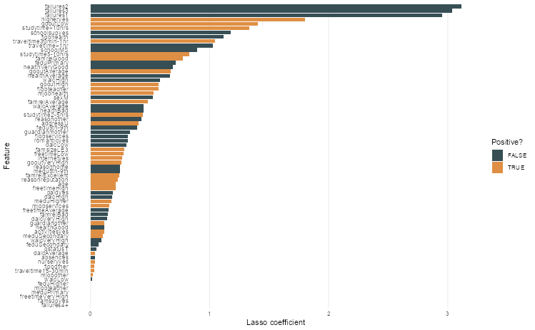
Step 4: Evaluate on the test set
Although a different model is used, the code for evaluating the model on the test set is exactly the same as earlier.
lasso_model |>
  augment(new_data = students_test) |>
  reg_metrics(truth = final_grade, estimate = .pred)
🗣️ CLASSROOM DISCUSSION:
Does this model represent an improvement on the linear model?
Compare the R-squared and RMSE values to our earlier multivariate model. Does the lasso provide better predictive performance or feature selection benefits?
(Bonus) Step 5: Experiment with different penalties
This is your chance to try out different penalties. Can you find a penalty that improves test set performance?
Let’s employ a nested tibbles approach to find better penalty values.
lasso <- partial(linear_reg, engine = "glmnet", mixture = 1)

preds <-
  crossing(
    penalty = c(0.0001, 0.001, 0.01, 0.1),
    nest(students_train, .key = "train"),
    nest(students_test, .key = "test")
  ) |>
  mutate(
    model = map(penalty, ~ lasso(penalty = .x)),
    fit = map2(model, train, ~ fit(.x, final_grade ~ ., data = .y)),
    augmented = map2(fit, test, ~ augment(.x, new_data = .y)),
    rmses = map(augmented, ~ rmse(.x, truth = final_grade, estimate = .pred))
  )

preds |>
  unnest(rmses) |>
  ggplot(aes(x = as.factor(penalty), y = .estimate, group = 1)) +
  geom_point() +
  geom_line(linetype = "dashed") +
  theme_minimal() +
  theme(
    panel.grid.minor = element_blank(),
    panel.grid.major.x = element_blank()
  ) +
  labs(x = "Penalty", y = "RMSE", title = "Test Set RMSE by Lasso Penalty")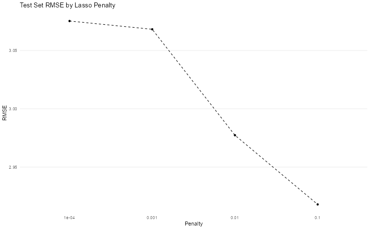
Which penalty value gives you the lowest RMSE? How do the coefficients change as you increase the penalty?
👉 NOTE: In labs 4 and 5, we are going to use a method called k-fold cross validation to systematically test different combinations of hyperparameters for models such as the lasso.
(Bonus) Challenge: Running multiple univariate regressions efficiently
🎯 YOUR CHALLENGE: Can you figure out how to run a univariate model for all features in the student dataset without creating 11 separate model objects?
Remember our univariate model earlier where we looked at final_grade ~ higher? Now we want to do the same thing for ALL features to see which individual variables are the strongest predictors of student performance.
The naive approach would be to copy-paste code 11 times and create 11 different model objects, but that’s inefficient and error-prone. Your job is to find a more elegant solution!
Your mission:
Figure out how to systematically run univariate regressions for each predictor variable and compare their performance.
Some things to think about:
- How can you automate the process of fitting multiple models?
- How will you store and compare the results?
- What’s the best way to visualize which features are most predictive?
Work in pairs and brainstorm different approaches!
You might consider:
- Loops (for loops, while loops)
- Functional programming (map functions)
- Advanced tidyverse techniques (nested tibbles)
- Or something completely different!
Questions to explore:
- Which single variable is the strongest predictor of student performance?
- Are there any surprisingly weak predictors?
- How do these univariate results compare to what you found significant in the multivariate model?
- Do the “best” univariate predictors match what you’d expect from theory?
Get creative and experiment!
There’s no single “right” way to solve this problem. Try different approaches, see what works, and don’t be afraid to ask for help when you get stuck.
Share your approach and findings on Slack! We want to see the different methods you came up with and which features you found most predictive.
library(tidymodels)
library(dplyr)
library(purrr)

# All predictors except the outcome
predictor_vars <- setdiff(names(students_train), "final_grade")

# Function to fit model and compute metrics
fit_metrics <- function(var) {
  formula <- as.formula(paste("final_grade ~", var))

  # Fit the model
  model <- linear_reg() %>%
    set_engine("lm") %>%
    fit(formula, data = students_train)

  # Compute predictions
  pred <- predict(model, students_train) %>% rename(.pred = .pred)
  results <- bind_cols(students_train, pred)

  # Compute RMSE and R² using yardstick
  metrics(results, truth = final_grade, estimate = .pred) %>%
    filter(.metric %in% c("rmse", "rsq")) %>%
    pivot_wider(names_from = .metric, values_from = .estimate) %>%
    mutate(predictor = var) %>%
    select(predictor, rsq, rmse)
}

# Apply to all predictors
univariate_results <- map_dfr(predictor_vars, fit_metrics)

# Sort by R², then RMSE
univariate_results %>%
  arrange(desc(rsq), rmse)
# A tibble: 30 × 3
   predictor    rsq  rmse
   <chr>      <dbl> <dbl>
 1 failures  0.192   2.90
 2 higher    0.115   3.04
 3 school    0.0876  3.08
 4 studytime 0.0687  3.11
 5 fedu      0.0615  3.13
 6 medu      0.0589  3.13
 7 mjob      0.0458  3.15
 8 address   0.0352  3.17
 9 reason    0.0350  3.17
10 walc      0.0330  3.17
# ℹ 20 more rows
# ℹ Use `print(n = ...)` to see more rows
On balance, failures seems to be the most predictive feature:
- it explains the most variance out of all features (though the variance explained is low ~19%)
- the RMSE obtained with this feature is also the lowest. We’re 2.9 points off on average on our grade predictions, i.e our predictions are off by about 14–15% of the total grade range (0–20). In practical terms, this means that if a student scored 16, the model would typically predict somewhere between roughly 13 and 19.
This also tells us that even the strongest univariate predictor leaves some noticeable uncertainty, which is expected when using just one feature.