🛣️ LSE DS202A 2025: Week 05 - Lab Roadmap

Author

The DS202 Team

Published

15 Sep 2025

🎯 Learning Outcomes

By the end of this lab, you will be able to:

Implement k-nearest neighbors with hyperparameter tuning
- Build k-NN models using tidymodels, understand how different k values affect decision boundaries, and use cross-validation to systematically optimize the number of neighbors for best performance.
Apply advanced cross-validation techniques for model evaluation
- Implement grouped cross-validation for clustered data structures, understand when to use different CV strategies, and interpret cross-validation results to select optimal hyperparameters.
Build and compare tree-based models
- Construct decision trees, random forests, and XGBoost models, visualize decision tree structures, and understand the trade-offs between interpretability and predictive performance across different ensemble methods.
Master hyperparameter tuning workflows
- Use tidymodels’ tune_grid() framework to systematically test different parameter combinations, create recipes for data preprocessing, and build complete workflows that combine model specifications with feature engineering steps.

📚 Preparation

Downloading the data sets

Download the lab’s `.qmd` notebook

Click on the link below to download the .qmd file for this lab. Save it in the DS202A folder you created in the first week. If you need a refresher on the setup, refer back to Part II of W01’s lab.

Import libraries

library("rpart.plot")
library("tidymodels")
library("tidyverse")
library("viridis")
library("rsample")
library("doParallel")
library("ranger")
library("xgboost")

Part I - k-Nearest Neighbors and Cross-Validation

Understanding decision boundaries in 2D feature space

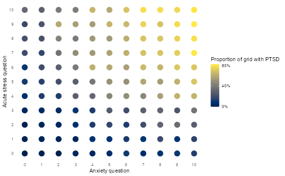
👨🏻‍🏫 TEACHING MOMENT: Your instructor will demonstrate how different machine learning algorithms create different decision boundaries in a 2D feature space using the PTSD data.

ptsd <-
  read_csv("data/ptsd-for-knn.csv") |>
  mutate(ptsd = as.factor(ptsd))

# Explore the feature space
ptsd |>
  group_by(anxiety, acute_stress) |>
  summarise(ptsd = mean(ptsd == 1, na.rm = TRUE)) |>
  ungroup() |>
  ggplot(aes(anxiety, acute_stress, colour = ptsd)) +
  geom_point(size = 5) +
  scale_x_continuous(breaks = 0:10) +
  scale_y_continuous(breaks = 0:10) +
  scale_colour_viridis(
    labels = percent,
    breaks = c(0, 0.4, 0.8),
    option = "cividis"
  ) +
  theme_minimal() +
  theme(panel.grid = element_blank()) +
  labs(
    x = "Anxiety question",
    y = "Acute stress question",
    colour = "Proportion of grid with PTSD"
  )

Challenge: Build a cross-validated k-NN model

Your mission: Create a k-NN model that uses 10-fold cross-validation to find the optimal number of neighbors for predicting PTSD.

Function glossary for this section:

initial_split() - split data into train/test
vfold_cv() - create cross-validation folds
nearest_neighbor() - specify k-NN model
tune() - mark parameters for tuning
recipe() - data preprocessing steps
step_normalize() - standardize features
workflow() - combine model + recipe
tune_grid() - perform cross-validation
collect_metrics() - extract CV results
select_best() - choose optimal parameters

Helpful resources:

Your tasks:

Split the data (75% train, 25% test, stratified by ptsd)
Create 10-fold CV on training data
Set up a k-NN model with neighbors = tune()
Create a recipe that normalizes features
Build a workflow combining model + recipe
Test different k values: c(1, 5, 10, 20, 50, 100, 200)
Visualize how performance changes with k
Select the best k and evaluate on test set


# Code here

Discussion questions:

Which k value performed best and why?
What happens with very small vs very large k values?
How do the cross-validation results compare to test set performance?

Part II - Tree-Based Models and Ensemble Methods

Understanding tree growth and ensembles

👨🏻‍🏫 TEACHING MOMENT: Your instructor will demonstrate:

How a basic decision tree splits data
How trees can grow and overfit
Introduction to ensemble methods (bagging, random forests)
How XGBoost incorporates learning from mistakes

Challenge: Compare tree-based models

Your mission: Build and compare three tree-based models for predicting childcare costs.

Function glossary for this section:

initial_split() - split data into train/test
sliding_period() - time-series CV with temporal ordering (⚠️requires the years to be converted from double to dates!)
decision_tree() - single decision tree
rand_forest() - random forest model
boost_tree() - XGBoost model
rpart.plot() - visualize decision tree
update_role() - assign variable roles in recipe

# ------------------------------------------------------------------------------
# 1. Load and prepare data
# ------------------------------------------------------------------------------

childcare <- read_csv("data/childcare-costs.csv")

# Split by time:
#  - Train: 2008–2016
#  - Test:  2017–2018
# We sort by year to preserve temporal order
# and create a Date column (`study_date`) for time-series cross-validation.

childcare_train <-
  childcare %>%
  filter(study_year <= 2016) %>%
  arrange(study_year) %>%
  mutate(study_date = as.Date(paste0(study_year, "-01-01")))

childcare_test <-
  childcare %>%
  filter(study_year > 2016) %>%
  mutate(study_date = as.Date(paste0(study_year, "-01-01")))

# -------------------------------------------------------# ------------------------------------------------------------------------------
# 2. Create time-series cross-validation folds
# ------------------------------------------------------------------------------
# We use sliding_period() instead of vfold_cv()
# to ensure no data leakage from future to past.
# The window expands each year, always predicting the next one.

childcare_cv <- sliding_period(
  childcare_train,
  index = study_date,
  period = "year",
  lookback = Inf,   # Expanding window: train on all prior years
  assess_stop = 1,  # Test on 1 future year
  step = 1          # Move forward 1 year each time
)

# This yields 8 folds (2008–2016)
length(childcare_cv$splits)

Predicting in New/Unseen Counties (Scenario B)

The approach above is appropriate when you want to predict future costs in counties you already have data for. However, if your goal is to predict costs in entirely new counties (e.g., expanding to new geographic markets), you need to combine time-series CV with county grouping:

library(tidyverse)
library(rsample)

# --- 1. Sample holdout counties once (never used in training) ----------
set.seed(123)
holdout_counties <- childcare_train %>%
  distinct(county_name) %>%
  slice_sample(prop = 0.2) %>%
  pull(county_name)

# --- 2. Build expanding-window time folds with fixed holdout counties --
val_years <- 2013:2016

childcare_cv_tbl <- tibble(val_year = val_years) %>%
  mutate(
    splits = map(val_year, \(year) {
      make_splits(
        list(
          # Train: all years before validation year, excluding holdout counties
          analysis = which(
            childcare_train$study_year < year &
              !(childcare_train$county_name %in% holdout_counties)
          ),
          # Validate: current year, only holdout counties
          assessment = which(
            childcare_train$study_year == year &
              childcare_train$county_name %in% holdout_counties
          )
        ),
        data = childcare_train
      )
    }),
    id = glue::glue("Year_{val_year}")
  )

# --- 3. Convert to a valid rset object (tidymodels-compatible) ----------
childcare_cv <- new_rset(
  splits = childcare_cv_tbl$splits,
  ids    = childcare_cv_tbl$id,
  attrib = tibble(val_year = childcare_cv_tbl$val_year),
  subclass = c("manual_rset", "rset")
)

childcare_cv

What this creates:

Fold 1: Train on 2008-2012 (80% of counties) → Validate on 2013 (20% holdout counties)
Fold 2: Train on 2008-2013 (80% of counties) → Validate on 2014 (20% holdout counties)
Fold 3: Train on 2008-2014 (80% of counties) → Validate on 2015 (20% holdout counties)
Fold 4: Train on 2008-2015 (80% of counties) → Validate on 2016 (20% holdout counties)

This ensures:

No time leakage (always train on past, validate on future)
No county leakage (holdout counties never appear in training)
True generalization to new geographic areas testing
Expanding window mimics realistic deployment (more training data over time)

Now that we’ve loaded the data and set the cross-validation, let’s write a pre-processing recipe:

# ------------------------------------------------------------------------------
# 3. Recipe: preprocessing pipeline
# ------------------------------------------------------------------------------
# We specify our modeling formula and tell tidymodels which variables
# should NOT be used as predictors (like county/state identifiers or study_date/study_year).

childcare_rec <-
  recipe(mcsa ~ ., data = childcare_train) %>%
  update_role(starts_with(c("county", "state")), new_role = "id") %>%
  update_role(c("study_date","study_year"), new_role = "id")  # used only for CV indexing, not modeling

Task 1: Decision Tree

Build a simple decision tree and visualize it:


# Code here

Class discussion: What does the tree visualization show? Which variables are most important?

Task 2: Random Forest

Build a random forest with mtry = round(sqrt(52), 0) and trees = 1000:


# Code here

Task 3: XGBoost with hyperparameter tuning

Build an XGBoost model and tune the learning rate using these values: c(0.0001, 0.001, 0.01, 0.1, 0.2, 0.3):


# Code here

Task 4: Compare all models

Create a visualization comparing the RMSE of all three models on the test set.


# Code here

Final discussion:

Which model performed best and why?
What are the trade-offs between interpretability and performance?
When might you choose each type of model?

🎯 Learning Outcomes

📚 Preparation

Downloading the data sets

Download the lab’s .qmd notebook

Import libraries

Part I - k-Nearest Neighbors and Cross-Validation

Understanding decision boundaries in 2D feature space

Challenge: Build a cross-validated k-NN model

Function glossary for this section:

Helpful resources:

Your tasks:

Part II - Tree-Based Models and Ensemble Methods

Understanding tree growth and ensembles

Challenge: Compare tree-based models

Function glossary for this section:

Task 1: Decision Tree

Task 2: Random Forest

Task 3: XGBoost with hyperparameter tuning

Task 4: Compare all models

Download the lab’s `.qmd` notebook