
✅ A model solution for the W08 summative
What follows is a possible solution for the W08 summative. If you want to render the .qmd that was used to generate this page for yourselves, use the download button below:
Keep in mind that this is only one possible solution but, by no means, the only one!
# Load all libraries here; suppress warnings/messages globally via YAML above
library(tidyverse)
library(tidymodels)
library(janitor)
library(skimr)
library(ggcorrplot)
library(vip)
library(ggdist)
library(pdp)

set.seed(123)  # for reproducibility of splits/resampling
options(dplyr.summarise.inform = FALSE)- Make sure to load all your libraries in a single code chunk at the beginning of your file. It’s much cleaner than sprinkling loading commands throughout.
- Don’t include any executable
install.packages()commands in your file. This would prevent your.qmdfrom rendering. If you want your readers to know they need to install packages and which ones they should install, then simply include a plain Markdown note on this.
Data loading and preparation
Q1.1 Load the dataset into a DataFrame sleep
# Adjust the path as needed for your setup
sleep <- read_csv("../../data/Sleep_health_and_lifestyle_dataset.csv", show_col_types = FALSE) %>%
  clean_names()

glimpse(sleep)
Rows: 374
Columns: 13
$ person_id               <dbl> 1, 2, 3, 4, 5, 6, 7, 8, 9, 10, 11, 12, 13, 14,…
$ gender                  <chr> "Male", "Male", "Male", "Male", "Male", "Male"…
$ age                     <dbl> 27, 28, 28, 28, 28, 28, 29, 29, 29, 29, 29, 29…
$ occupation              <chr> "Software Engineer", "Doctor", "Doctor", "Sale…
$ sleep_duration          <dbl> 6.1, 6.2, 6.2, 5.9, 5.9, 5.9, 6.3, 7.8, 7.8, 7…
$ quality_of_sleep        <dbl> 6, 6, 6, 4, 4, 4, 6, 7, 7, 7, 6, 7, 6, 6, 6, 6…
$ physical_activity_level <dbl> 42, 60, 60, 30, 30, 30, 40, 75, 75, 75, 30, 75…
$ stress_level            <dbl> 6, 8, 8, 8, 8, 8, 7, 6, 6, 6, 8, 6, 8, 8, 8, 8…
$ bmi_category            <chr> "Overweight", "Normal", "Normal", "Obese", "Ob…
$ blood_pressure          <chr> "126/83", "125/80", "125/80", "140/90", "140/9…
$ heart_rate              <dbl> 77, 75, 75, 85, 85, 85, 82, 70, 70, 70, 70, 70…
$ daily_steps             <dbl> 4200, 10000, 10000, 3000, 3000, 3000, 3500, 80…
$ sleep_disorder          <chr> "None", "None", "None", "Sleep Apnea", "Sleep …
We load the CSV file into a tibble called sleep and clean the column names to snake_case for easier use with tidyverse/tidymodels. The dataset includes demographic variables (e.g. age, gender, occupation), lifestyle variables (e.g. physical_activity_level, daily_steps, stress_level), and sleep-related outcomes such as sleep_duration, quality_of_sleep, and sleep_disorder.
The person_id column (if present) is an identifier and should not be used as a predictor in modelling.
When loading the dataset, use a relative file path, and make sure the file is stored in your repository in the same structure as in the material you submit.
Absolute paths (e.g., "/Users/alex/Desktop/data/...") will only work on your own machine and break reproducibility. Relative paths ensure that your .qmd runs correctly on any computer without modification.
Part 1: Data Exploration (15 marks)
Q1.2 Explore and visualise the data
1.2.a Correlations with sleep duration
We want to try and check which variables are most strongly correlated with sleep duration so we construct a correlation matrix based on the datasets’ numeric features (correlation is meaningless for categorical features!)
# Select numeric variables for correlation
sleep_numeric <- sleep %>%
  select(where(is.numeric)) %>%
  select(-person_id)  # drop ID if present

# Correlation matrix
cor_sleep <- cor(sleep_numeric, use = "pairwise.complete.obs")

# Focus on correlations with sleep_duration
cor_sleep[,"sleep_duration"] %>% sort(decreasing = TRUE)
         sleep_duration        quality_of_sleep                     age
             1.00000000              0.88321300              0.34470936
physical_activity_level             daily_steps              heart_rate
             0.21236031             -0.03953254             -0.51645489
           stress_level
            -0.81102303
We visualise these correlations as a heatmap.
# Visual correlation plot
ggcorrplot(
  cor_sleep,
  hc.order = TRUE,
  type = "lower",
  lab = TRUE,            # show correlation labels
  lab_size = 3,
  outline.col = "white",
  colors = c("#8CDEDC", "white", "#841C26")
) +
  theme(
    axis.text.x = element_text(angle = 90, hjust = 1)
  )
The correlation vector and heatmap help us identify which numeric variables show meaningful linear associations with sleep_duration.
From the matrix we observe:
Strong positive association between sleep_duration and quality_of_sleep (≈ 0.88). This is expected: participants who report higher sleep quality tend to also report sleeping more hours. Because both variables reflect aspects of sleep, some degree of correlation is structurally built into the dataset.
Moderate positive associations with daily_steps (≈ 0.21) and age (≈ 0.34). These suggest that, in this synthetic sample, people who take more daily steps or who are slightly older report somewhat longer sleep. These correlations are modest and should not be over-interpreted.
Near-zero associations with physical_activity_level (≈ −0.04). Despite intuition that more activity might improve sleep duration, the synthetic data does not show a meaningful linear relationship here.
Moderate negative associations with stress_level (≈ −0.52). Participants with higher stress levels tend to sleep fewer hours. This is consistent with real-world findings, but we must remember that correlation does not indicate cause.
Weak negative associations with heart_rate (≈ −0.23). This suggests that higher resting heart rate is slightly associated with shorter sleep, though again the relationship is weak.
Overall, the strongest signals relate to quality_of_sleep and stress_level, which makes substantive sense: both are conceptually tied to sleep outcomes. Other numeric variables exhibit weak correlations, indicating the relationship between lifestyle factors and sleep duration is complex and potentially non-linear.
As always, correlations capture association rather than causation, so these patterns should be used to motivate modelling decisions (e.g., variable selection) rather than to draw causal conclusions.
1.2.b Subgroup differences
Sleep duration by gender
We begin by examining whether sleep duration differs across genders.
sleep %>% count(gender)# A tibble: 2 × 2
gender n
<chr> <int>
1 Female 185
2 Male 189The dataset includes 185 females and 189 males, providing a balanced sample for comparison.
Distribution plot (density)
sleep %>%
  ggplot(aes(x = sleep_duration, fill = gender, colour = gender)) +
  geom_density(alpha = 0.4, size = 1) +
  scale_fill_brewer(palette = "Pastel1") +
  scale_colour_brewer(palette = "Dark2") +
  labs(
    title = "Sleep Duration Distributions by Gender",
    subtitle = "Women show slightly greater variability, \n while both groups share similar medians around 7–7.5 hours",
    x = "Sleep duration (hours)",
    y = "Density"
  ) +
  theme_minimal(base_size = 14)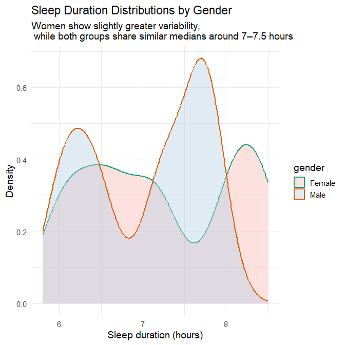
Half-violin + boxplot hybrid
sleep %>%
  ggplot(aes(x = gender, y = sleep_duration, fill = gender)) +
  stat_halfeye(
    adjust = 0.6,
    width = 0.7,
    .width = 0,
    justification = -0.3,
    alpha = 0.6
  ) +
  geom_boxplot(
    width = 0.25,
    outlier.shape = NA,
    alpha = 0.9,
    colour = "black"
  ) +
  scale_fill_brewer(palette = "Pastel1") +
  labs(
    title = "Distribution of Sleep Duration by Gender",
    subtitle = "Medians are nearly identical, \n but women display a broader spread of sleep durations",
    x = "Gender",
    y = "Sleep duration (hours)"
  ) +
  theme_minimal(base_size = 14) +
  theme(legend.position = "none")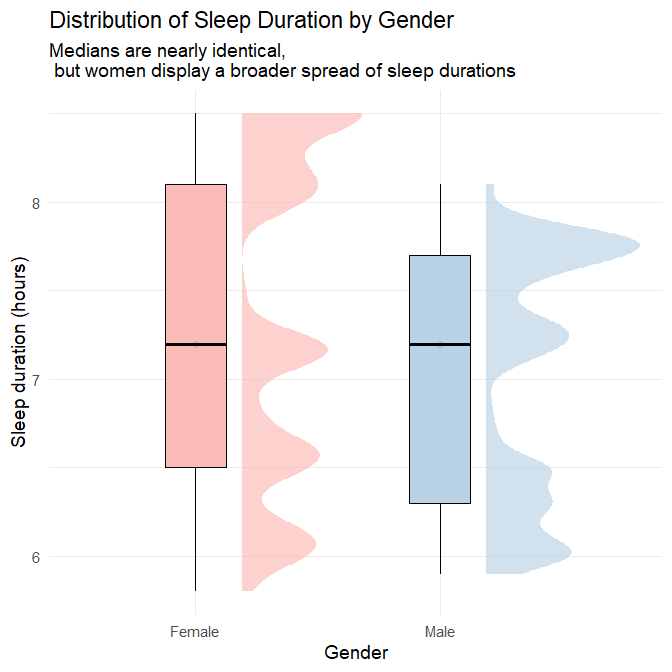
Plots’ interpretation
The two visualisations together provide a detailed and nuanced comparison of sleep patterns between genders.
1. Central tendency
Both the density plot and the half-violin/boxplot hybrid show that:
- Men and women share a very similar median sleep duration, slightly above 7 hours.
- The bulk of observations for both genders fall between 7 and 7.5 hours.
- There is no evidence of a systematic shift in typical sleep duration between genders.
This indicates that average sleep duration does not differ meaningfully by gender in this dataset.
2. Variability, spread, and range
The full distributions reveal subtleties that would be invisible if we looked only at the median:
Women show slightly greater variability in sleep duration, as indicated by:
- a broader density curve,
- a longer left-tail (more short sleepers),
- a longer right-tail (more long sleepers),
- a wider half-violin shape,
- both lower minimum and higher maximum values than men.
Men exhibit a more concentrated pattern, reflected in:
- a noticeably “peakier” density curve,
- a narrower half-violin span,
- fewer extreme values on either end.
This difference is subtle, but consistent across both visualisations: women’s sleep durations vary more widely, whereas men cluster more tightly around the median.
3. Shape of distributions
- The female density curve is flatter and more spread out, indicating more heterogeneity.
- The male density curve is sharper, reflecting greater uniformity.
- Both distributions remain unimodal, centred around the same dominant peak.
These shapes confirm that the difference between genders lies not in typical sleep, but in how consistently they sleep.
Take-away
There is no meaningful difference in central tendency (mean or median) between men and women in this dataset. However:
- Women show a broader range, implying more night-to-night or individual-to-individual variation.
- Men show more consistency, with most values clustered near the median.
This illustrates why EDA should examine distribution shape, not just summary statistics.
Explanatory context
Although this dataset is synthetic, subtle gender differences in sleep variability have been documented in real-world sleep research. One consistent finding is that women experience more sleep disturbances and insomnia symptoms, even when total sleep duration is similar to men (Zhang and Wing 2006) (R. H. Y. Li et al. 2002) . Such disturbances can increase night-to-night variability in overall sleep hours.
Research on couples also shows that women are more susceptible to sleep-maintenance disruptions linked to household or partner-related factors, such as nocturnal awakenings and mismatched routines (Meadows and Arber 2012). While this research does not directly address total sleep duration, it illustrates how social patterns within households can produce less consistent nightly sleep for women.
Broader sociological research reinforces this picture. (Burgard and Ailshire 2013) show that women often have less discretionary time available for sleep due to unequal divisions of domestic labour, childcare responsibilities, and work–family conflict. These social constraints can lead to more irregular sleep schedules, even when average total sleep time is similar.
Additionally, caregiving responsibilities — still disproportionately carried by women — have been linked to increased sleep difficulties and irregular sleep patterns (Straat, Willems, and Bracke 2020) . Women also tend to experience greater variability in daily stress exposure (Almeida and Kessler 1998), and stress is a well-established contributor to fragmented and inconsistent sleep (Akerstedt 2006).
Taken together, these findings support the idea that greater variability in women’s sleep can arise from a combination of:
- higher rates of insomnia and nocturnal disturbances,
- greater exposure to household or partner-related sleep disruptions,
- unequal caregiving and domestic responsibilities,
- and stress-related sleep fragmentation.
These mechanisms do not imply biological determinism; rather, they reflect well-documented social, behavioural, and psychological factors that may help explain the pattern observed in this dataset.
Sleep Duration by Age Group
Creating age groups
We begin by creating an age_group variable, since the dataset does not contain one by default. Here we define two broad groups commonly used in sleep epidemiology: 26–40 and 41–60.
sleep <- sleep %>%
  mutate(
    age_group = case_when(
      age >= 26 & age <= 40 ~ "26–40",
      age >= 41 & age <= 60 ~ "41–60",
      TRUE ~ NA_character_
    ),
    age_group = factor(age_group, levels = c("26–40", "41–60"))
  )
Age group counts
We check how participants are distributed across age groups.
sleep %>%
  count(age_group)
# A tibble: 2 × 2
age_group n
<fct> <int>
1 26–40 165
2 41–60 209Comment: The age groups are not perfectly balanced (165 vs. 209 participants), but both groups have sufficiently large samples to support meaningful comparison.
Plot: Sleep duration by age group
We now visualise the distribution of sleep duration for each age group using a violin–boxplot combination, which shows both central tendencies and distribution shapes.
sleep %>%
  ggplot(aes(x = age_group, y = sleep_duration, fill = age_group)) +
  geom_violin(alpha = 0.4, trim = FALSE, colour = "grey30") +
  geom_boxplot(width = 0.18, alpha = 0.9, outlier.shape = NA, colour = "grey20") +
  scale_fill_brewer(palette = "Pastel2") +
  labs(
    title    = "Sleep Duration by Age Group",
    subtitle = "Median sleep is similar across age groups, \n but 41–60 year-olds show greater variability",
    x        = "Age group",
    y        = "Sleep duration (hours)"
  ) +
  theme_minimal(base_size = 14) +
  theme(legend.position = "none")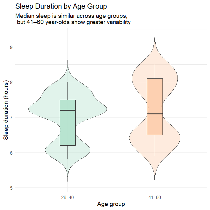
Interpretation
The median sleep duration is nearly identical across the two age groups, with both centred slightly above seven hours. This suggests that, at the population level, typical sleep quantity remains relatively stable from early adulthood into midlife.
What differs more visibly is the shape of the distributions:
Adults aged 26–40 show a tighter clustering of sleep durations, with most individuals sleeping between 6.5 and 8 hours.
Adults aged 41–60 display a broader spread, including:
more short sleepers (below ~6 hours), and
more long sleepers (above ~8.5 hours).
This pattern indicates that while average sleep duration is consistent, sleep behaviour becomes more heterogeneous in later adulthood, with a subset of individuals experiencing markedly shorter or longer sleep durations than the typical range.
Explanatory context
Research on sleep and ageing shows patterns that help contextualise this distribution:
Normal ageing involves changes in sleep continuity, including increased awakenings and more fragmented sleep (J. Li, Vitiello, and Gooneratne 2018). These changes do not necessarily reduce average sleep duration but often introduce greater night-to-night variability, consistent with our broader spread in the older group.
Longer-than-average sleep duration in older adults has been associated with elevated risk of later cognitive decline (Ma et al. 2020) and dementia in prospective analyses (Fan et al. 2019) (Bulycheva et al. 2024). This does not imply dementia within this synthetic dataset, but it illustrates why a subgroup of long sleepers is more plausible in older than younger adults.
Together, these findings support the interpretation that the wider distribution in the 41–60 group is consistent with known age-related variability in sleep patterns.
Sleep Duration by Occupation
Occupation counts
We first examine how many individuals represent each occupational category.
sleep %>%
  count(occupation, sort = TRUE)
# A tibble: 11 × 2
occupation n
<chr> <int>
1 Nurse 73
2 Doctor 71
3 Engineer 63
4 Lawyer 47
5 Teacher 40
6 Accountant 37
7 Salesperson 32
8 Scientist 4
9 Software Engineer 4
10 Sales Representative 2
11 Manager 1Comment: Some occupations (e.g., nurses, doctors, engineers) have large sample sizes, while others (e.g., scientists, sales representatives, manager) contain very few participants. This uneven representation must be considered when interpreting differences.
Plot: Sleep duration by occupation
We visualise occupational differences, ordering occupations by median sleep duration.
sleep %>%
  mutate(occupation = fct_reorder(occupation, sleep_duration, .fun = median)) %>%
  ggplot(aes(x = sleep_duration, y = occupation, fill = occupation)) +
  geom_boxplot(alpha = 0.7, outlier.shape = NA, colour = "grey20") +
  geom_jitter(height = 0.1, alpha = 0.6, size = 1) +
  scale_fill_brewer(palette = "Set3") +
  labs(
    title    = "Sleep Duration by Occupation",
    subtitle = "Interpret patterns cautiously:\n sample sizes vary widely across occupations",
    x        = "Sleep duration (hours)",
    y        = "Occupation"
  ) +
  theme_minimal(base_size = 14) +
  theme(legend.position = "none")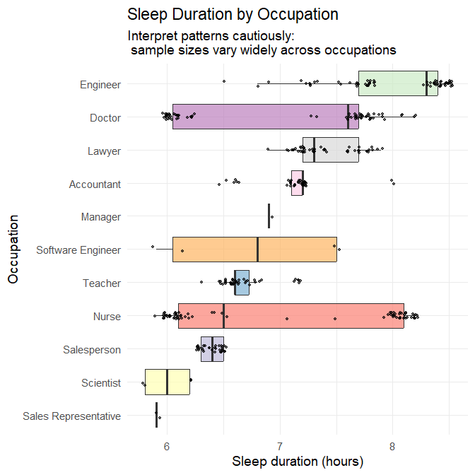
Interpretation
Well-represented occupations
For occupations with large sample sizes (N ≳ 30), meaningful patterns emerge:
- Nurses show a wide distribution of sleep durations, ranging roughly 6–8.5 hours.
- Doctors also show substantial variability.
- Teachers, accountants, engineers, lawyers, and salespeople show narrower distributions centred near 7 hours.
These patterns align with differences in schedule regularity: shift-based professions such as nursing and medicine exhibit more varied sleep timing and duration, whereas more consistent daytime roles produce tighter clustering.
Under-represented occupations
Occupations with N < 10 cannot support reliable inference. Their boxplots are largely driven by individual values, and observed variation should not be overinterpreted.
Take-away
Occupational differences appear consistent with known impacts of work schedules on sleep, but unequal sample sizes strongly limit interpretability for several categories.
Explanatory context
The observed patterns align with robust occupational health findings:
- Systematic reviews describe shift work as associated with shorter and more irregular sleep, circadian disruption, and increased sleepiness (Harrington 1994) (Wu et al. 2022).
- Nurses working 12-hour shifts average only ~5.5 hours of sleep between shifts, experience cumulative fatigue, and display increased sleepiness across consecutive workdays (Geiger-Brown et al. 2012).
- Limiting extended shifts in medical interns significantly increases total sleep time and reduces attentional failures (Lockley et al. 2004).
- Observational work shows that extended or irregular shifts in medical trainees lead to substantial variability in sleep (Basner et al. 2017).
These findings support the interpretation that wide sleep variability in nurses and doctors is credible, while categories with very small sample sizes remain unreliable for inference.
Sleep Duration by Sleep Disorder Status
Sleep disorder counts
We check the representation of each disorder category.
sleep %>%
  count(sleep_disorder)
# A tibble: 3 × 2
sleep_disorder n
<chr> <int>
1 Insomnia 77
2 None 219
3 Sleep Apnea 78Comment: All three groups (None, Insomnia, Sleep Apnea) are well represented. Unlike the occupation variable, we can interpret differences with confidence.
Plot: Sleep duration by disorder
sleep %>%
  mutate(sleep_disorder = fct_relevel(sleep_disorder, "None", "Insomnia", "Sleep Apnea")) %>%
  ggplot(aes(x = sleep_disorder, y = sleep_duration, fill = sleep_disorder)) +
  geom_violin(alpha = 0.4, trim = FALSE, colour = "grey30") +
  geom_boxplot(width = 0.18, alpha = 0.9, outlier.shape = NA, colour = "grey20") +
  scale_fill_brewer(palette = "Pastel1") +
  labs(
    title    = "Sleep Duration by Sleep Disorder Status",
    subtitle = "Insomnia is associated with shorter sleep;\n sleep apnea shows the broadest variability",
    x        = "Sleep disorder",
    y        = "Sleep duration (hours)"
  ) +
  theme_minimal(base_size = 14) +
  theme(legend.position = "none")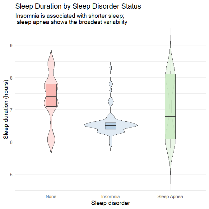
Interpretation
No disorder: Participants without sleep disorders sleep the most and show moderate variability.
Insomnia: This group exhibits the lowest median sleep duration (~6.4 hours) with a narrow, left-shifted distribution. Most individuals cluster between 6–6.8 hours, reflecting the diagnostic hallmark of insomnia: difficulty initiating or maintaining sleep.
Sleep apnea: Median sleep duration is somewhat lower than the “no disorder” group, but the distribution is notably wide, with both short and long sleepers. This reflects:
- fragmented sleep due to repeated apneic events
- compensatory longer sleep in some individuals due to excessive daytime sleepiness
Take-away
Sleep disorder status is highly informative: insomnia predicts consistently shortened sleep, while sleep apnea predicts variable and disrupted sleep patterns.
Explanatory context
Insomnia is defined by difficulty initiating or maintaining sleep, typically resulting in reduced, non-restorative sleep (American Psychiatric Association 2013) (Roth 2007) (American Academy of Sleep Medicine 2014). This aligns neatly with the narrow, reduced sleep durations seen in the insomnia group.
Obstructive sleep apnea is characterised by repeated upper-airway obstruction, oxygen desaturation, and recurrent arousals, producing fragmented sleep (Jordan, McSharry, and Malhotra 2014). Such fragmentation yields both:
- short sleep (due to awakenings) and
- longer sleep in some cases (due to compensatory hypersomnia).
These documented clinical patterns strongly support the observed distributions.
1.2.c Multivariable Plot: Sleep Duration, Stress Level, and Physical Activity
Understanding how sleep duration relates to a single predictor is informative, but real-world behaviours are typically shaped by multiple factors at once. In this section, we examine a multivariable relationship by exploring how:
- sleep duration varies with
- stress level (primary predictor), while
- physical activity is represented through colour-coded activity bands.
This visualisation helps us assess whether physical activity appears to modify or contextualise the relationship between stress and sleep.
Step 1 — Create a banded physical-activity variable
Before plotting, we organise physical activity into meaningful bands. This avoids the visual clutter of colouring by dozens of distinct numeric values and allows clearer interpretation.
sleep <- sleep %>%
  mutate(
    activity_band = case_when(
      physical_activity_level < 45 ~ "Low activity (<45 min)",
      physical_activity_level < 70 ~ "Moderate activity (45–69 min)",
      TRUE                         ~ "High activity (≥70 min)"
    ) %>% factor(
      levels = c(
        "Low activity (<45 min)",
        "Moderate activity (45–69 min)",
        "High activity (≥70 min)"
      )
    )
  )
Step 2 — Inspect how many participants fall into each activity band
We check the distribution across bands to ensure each category has enough observations for meaningful interpretation.
sleep %>%
  count(activity_band)
# A tibble: 3 × 2
activity_band n
<fct> <int>
1 Low activity (<45 min) 82
2 Moderate activity (45–69 min) 151
3 High activity (≥70 min) 141Comment:
All three activity bands (Low activity, Moderate activity, High activity) are well represented. We can interpret the coloured clusters with confidence.
Step 3 — Create the multivariable plot
We now plot sleep duration against stress level, colouring the points according to the newly created activity bands. A linear smoothing line summarises the overall stress–sleep association.
sleep %>%
  ggplot(aes(x = stress_level,
             y = sleep_duration,
             colour = activity_band)) +
  geom_point(size = 2, alpha = 0.8) +
  geom_smooth(method = "lm", se = FALSE, colour = "black") +
  scale_colour_manual(
    values = c(
      "Low activity (<45 min)"        = "#2A9D8F",
      "Moderate activity (45–69 min)" = "#E76F51",
      "High activity (≥70 min)"       = "#6A5ACD"
    )
  ) +
  labs(
    title = "Sleep Duration vs Stress Level",
    subtitle = "Higher stress is associated with shorter sleep; higher physical activity\n corresponds to slightly longer sleep at similar stress levels",
    x = "Stress level (1–10 scale)",
    y = "Sleep duration (hours)",
    colour = "Activity band"
  ) +
  theme_minimal(base_size = 14)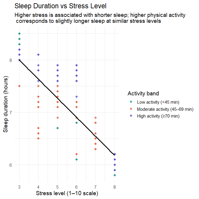
Interpretation
1. Main association: stress level and sleep duration
The fitted line shows a clear negative association:
- As stress level increases, sleep duration decreases.
- The downward trend is smooth and approximately linear across the observed range.
- The clustering of points around the line suggests that stress is a relatively strong predictor of sleep duration in this dataset.
This indicates that stress is likely to play a major role in the regression modelling that follows.
2. Added insight from physical activity
The coloured activity bands add a second dimension:
- Participants in the high-activity band (≥70 min/day) tend to appear slightly higher on the sleep-duration axis at each stress level.
- Participants in the low-activity band (<45 min/day) tend to appear lower.
- The moderate-activity band falls in between, with some overlap.
These differences are modest but consistent:
Even at the same stress level, participants with higher physical activity tend to sleep slightly longer than those with lower activity.
This pattern reflects two complementary strands of evidence:
- Regular physical activity is associated with better sleep onset and sleep continuity, and with improvements in overall sleep quality (Kredlow et al. 2015) (Kline 2014).
- Physical activity has been shown to reduce stress-related neuroendocrine activation and improve resilience to chronic stress, which may offer a plausible mechanism for the slightly longer sleep observed among more active individuals in this dataset (Tsatsoulis and Fountoulakis 2006).
Together, these findings offer a behavioural and physiological explanation for the vertical separation seen between activity bands.
3. Full multivariable pattern
Considering both predictors jointly:
- Stress level exerts the strongest influence on sleep duration.
- Physical activity introduces a secondary, “buffering” pattern, where active individuals tend to sleep slightly longer.
- The negative association between stress and sleep remains present across all activity bands.
This mirrors the type of structure we will model statistically in Part 2.
Key takeaway
This multivariable plot shows that:
- Stress is a strong and consistently negative predictor of sleep duration.
- Physical activity provides a modest buffering effect, with more active participants sleeping slightly longer at similar stress levels.
- Combining predictors visually yields a richer understanding of the structure in the data—insights that will inform later modelling decisions.
1.2.d Missing Data and Anomalies
Before moving on to modelling, we must ensure the dataset is complete and free from problematic anomalies. Missingness and outliers can influence regression and classification in undesirable ways (e.g., biased coefficients, unstable splits, inflated errors). In this dataset, both steps are straightforward but still essential.
1. Checking for Missing Data
We first compute the number of missing values in each column:
sleep %>%
  summarise(across(everything(), ~ sum(is.na(.)))) %>%
  pivot_longer(everything(),
               names_to = "variable",
               values_to = "n_missing")
# A tibble: 15 × 2
variable n_missing
<chr> <int>
1 person_id 0
2 gender 0
3 age 0
4 occupation 0
5 sleep_duration 0
6 quality_of_sleep 0
7 physical_activity_level 0
8 stress_level 0
9 bmi_category 0
10 blood_pressure 0
11 heart_rate 0
12 daily_steps 0
13 sleep_disorder 0
14 age_group 0
15 activity_band 0We also examine summary statistics and variable types:
skim(sleep)── Data Summary ────────────────────────
Values
Name sleep
Number of rows 374
Number of columns 15
_______________________
Column type frequency:
character 5
factor 2
numeric 8
________________________
Group variables None
── Variable type: character ────────────────────────────────────────────────────
skim_variable n_missing complete_rate min max empty n_unique whitespace
1 gender 0 1 4 6 0 2 0
2 occupation 0 1 5 20 0 11 0
3 bmi_category 0 1 5 13 0 4 0
4 blood_pressure 0 1 6 6 0 25 0
5 sleep_disorder 0 1 4 11 0 3 0
── Variable type: factor ───────────────────────────────────────────────────────
skim_variable n_missing complete_rate ordered n_unique
1 age_group 0 1 FALSE 2
2 activity_band 0 1 FALSE 3
top_counts
1 41–: 209, 26–: 165
2 Mod: 151, Hig: 141, Low: 82
── Variable type: numeric ──────────────────────────────────────────────────────
skim_variable n_missing complete_rate mean sd p0 p25
1 person_id 0 1 188. 108. 1 94.2
2 age 0 1 42.2 8.67 27 35.2
3 sleep_duration 0 1 7.13 0.796 5.8 6.4
4 quality_of_sleep 0 1 7.31 1.20 4 6
5 physical_activity_level 0 1 59.2 20.8 30 45
6 stress_level 0 1 5.39 1.77 3 4
7 heart_rate 0 1 70.2 4.14 65 68
8 daily_steps 0 1 6817. 1618. 3000 5600
p50 p75 p100 hist
1 188. 281. 374 ▇▇▇▇▇
2 43 50 59 ▆▆▇▃▅
3 7.2 7.8 8.5 ▇▆▇▇▆
4 7 8 9 ▁▇▆▇▅
5 60 75 90 ▇▇▇▇▇
6 5 7 8 ▇▃▂▃▃
7 70 72 86 ▇▇▂▁▁
8 7000 8000 10000 ▁▅▇▆▂Result:
This synthetic Kaggle dataset contains no missing values in any variable. This is unusual for real-world datasets but expected for synthetic data.
2. Preparing for anomaly detection: Split blood pressure into numeric components
The variable blood_pressure is stored as a single string in "systolic/diastolic" format. To detect anomalies properly — and to model the predictors later — it is preferable to split this into two numeric columns.
Reformat blood pressure:
sleep <- sleep %>%
  separate(blood_pressure,
           into = c("bp_systolic", "bp_diastolic"),
           sep = "/",
           convert = TRUE)
Why this matters:
- A string variable cannot be used directly in regression or classification.
- Systolic and diastolic pressures have different physiological interpretations, so treating them separately is more meaningful.
- Splitting allows us to check each component for anomalies (e.g., systolic < 90 or > 200 mmHg).
We now have two clean numeric predictors: sleep$bp_systolic and sleep$bp_diastolic.
3. Checking for anomalies
Even without missing data, numerical variables may contain values that fall outside expected physiological or behavioural ranges. In real-world datasets, anomalies often arise from device errors, data-entry mistakes, unit mix-ups, or genuinely unusual human situations. We therefore inspect each major numeric variable in turn to understand whether any values require attention before modelling.
3.1 Sleep duration
Code: Examine the range of sleep duration
summary(sleep$sleep_duration) Min. 1st Qu. Median Mean 3rd Qu. Max.
5.800 6.400 7.200 7.132 7.800 8.500Interpretation
All sleep durations fall between 5.8 and 8.5 hours, which represents a typical mid-range adult sleep pattern.
However, in real-world sleep-health datasets, we normally find a much broader and more irregular spread, including:
Very short sleep (< 3 hours) — which is not necessarily an anomaly. It can occur with:
- night-shift work
- medical trainees working overnight
- caregiving responsibilities
- acute or chronic insomnia
- high stress or crisis situations
- severe mental health episodes
Very long sleep (> 11–12 hours) — which may arise in:
- hypersomnia disorders
- bipolar depressive episodes
- neurological illness
- chronic fatigue
- recovery after prolonged sleep deprivation
- sedating medications
Thus, the absence of both unusually short and unusually long sleepers — and the smooth, tightly bounded distribution — strongly suggests synthetic generation rather than natural variation.
In real datasets, such extreme values would require contextual judgment rather than automatic removal.
3.2 Heart rate
Code: Examine resting heart rate values
summary(sleep$heart_rate) Min. 1st Qu. Median Mean 3rd Qu. Max.
65.00 68.00 70.00 70.17 72.00 86.00Interpretation
All heart rates fall between 65 and 86 bpm, entirely within the expected resting range for adults (~60–100 bpm).
In real physiological datasets, we would often expect:
Bradycardia (< 50 bpm) Seen in endurance athletes, individuals on certain medications, or those with conduction abnormalities.
Tachycardia (> 110 bpm) Common in cases of illness, anxiety, pain, dehydration, stimulant use, endocrine disorders, or device misreads.
The tight clustering in this dataset — without unusually low or high values — again signals synthetic smoothing.
3.3 Daily steps
Code: Examine step-count distribution
summary(sleep$daily_steps) Min. 1st Qu. Median Mean 3rd Qu. Max.
3000 5600 7000 6817 8000 10000Interpretation
All values lie within a plausible human activity range (3,000–10,000 steps per day). However, real activity datasets usually include:
- very low step counts (< 500/day) — common among people with limited mobility or during illness,
- very high values (> 20,000) — typical for athletes, healthcare workers, or delivery staff,
- implausible values (> 50,000) — often indicating device malfunction or unit confusion.
The capped maximum of exactly 10,000 steps, a culturally recognised “goal,” further suggests synthetic construction rather than observed behaviour.
3.4 Physical activity level (minutes/day)
Code: Examine daily activity minutes
summary(sleep$physical_activity_level) Min. 1st Qu. Median Mean 3rd Qu. Max.
30.00 45.00 60.00 59.17 75.00 90.00Interpretation
All physical-activity values fall between 30 and 90 minutes, which is reasonable.
However, true observational datasets almost always include:
- nearly sedentary days (0–10 minutes)
- occasional extreme activity (> 150 minutes/day)
- misreported values (e.g., “300 minutes” instead of “30”)
- device-originated artefacts
The absence of both low-activity and high-activity individuals makes the distribution unnaturally regular — again consistent with synthetic data.
3.5 Blood pressure (after splitting)
Code: Examine systolic and diastolic pressure
summary(sleep$bp_systolic)
summary(sleep$bp_diastolic)
> summary(sleep$bp_systolic)
Min. 1st Qu. Median Mean 3rd Qu. Max.
115.0 125.0 130.0 128.6 135.0 142.0
> summary(sleep$bp_diastolic)
Min. 1st Qu. Median Mean 3rd Qu. Max.
75.00 80.00 85.00 84.65 90.00 95.00Interpretation
These values span typical normal and mildly hypertensive ranges.
Real-world blood pressure data usually include:
hypotensive values (< 90/60)
severely hypertensive values (> 180/120)
measurement artefacts, such as:
- reversed values (e.g., “85/140”),
- truncated values (e.g., “120/8”),
- device-driven rounding or plateauing.
The absence of such irregularities again indicates a synthetic dataset.
🧠 Final Interpretation and implications for modelling
Across all numeric variables, we observe a consistent pattern:
- All values fall within realistic adult ranges,
- but the distributions are unusually tight, smooth, and bounded,
- lacking the extremes, irregularities, measurement noise, and rare events typical of real observational data.
This strongly suggests that the dataset has been synthetically generated with constraints designed to produce “clean” values.
Why this matters for modelling
When we work with real-world sleep, lifestyle, or clinical datasets, anomaly-handling becomes a central part of the workflow:
- very short or very long sleep durations may be meaningful, not errors,
- extreme heart rates or blood pressures may indicate important subgroups,
- unusually low or high activity metrics may reflect occupational patterns or health conditions,
- anomalies may arise from measurement error and require correction or transformation.
In this dataset, because values have been artificially regularised, we can proceed directly into modelling without worrying about anomaly removal or variable transformation.
However, it is important to recognise that this is a special case: anomaly detection is a critical step in most applied machine learning and statistical modelling projects.
Part 2: Regression – Predicting Sleep Duration (35 marks)
Q2.1 Train–test split
Before fitting any regression models, we first create separate datasets for training (used to estimate the model and tune any necessary components) and testing (used only at the end to evaluate how well the model generalises to unseen data). It is essential that this split is performed before any modelling-specific preprocessing so that the test dataset remains a truly independent sample of new, unseen observations.
Code
set.seed(123)  # ensures reproducible random splitting

# Remove the EDA-only derived variables
sleep_reg <- sleep %>%
  select(-age_group, -activity_band)

# Create an 80/20 train–test split
sleep_split <- initial_split(sleep_reg, prop = 0.8)

sleep_train <- training(sleep_split)
sleep_test  <- testing(sleep_split)

nrow(sleep_train); nrow(sleep_test)[1] 299
[1] 75Interpretation
We use an 80% training / 20% testing split. This proportion provides:
- a training set large enough to estimate regression parameters reliably and to support internal resampling (e.g., cross-validation), and
- a test set sufficiently large to give an unbiased and reasonably stable estimate of out-of-sample performance.
Because the dataset is cross-sectional (not longitudinal, not hierarchical, and not time-ordered), a simple random split is appropriate. We specify a fixed set.seed() to ensure full reproducibility, guaranteeing that the same rows will appear in the training and test sets every time the analysis is run.
Stratification is commonly used when the outcome variable is categorical and imbalanced, such as in classification problems where one level is rare. However, stratification may also be applied to predictor variables, particularly when:
- there are important subgroups that are small,
- there is a risk that a purely random split might exclude those subgroups from the test set,
- or the analyst wants to ensure consistent representation of specific categories.
In this dataset, several variables could reasonably justify stratification:
1. Sleep disorder
The distribution is strongly imbalanced:
- None: 219
- Insomnia: 77
- Sleep Apnea: 78
Stratifying by sleep_disorder would ensure that both the training and test sets preserve a similar proportion of the three groups, which may be useful if we later wish to examine model performance across disorder types.
2. Occupation
This variable includes multiple extremely rare categories, including occupations with only 1–4 observations (“Manager,” “Sales Representative,” “Scientist,” “Software Engineer”). Stratification could prevent these rare occupations from disappearing entirely from either dataset. This may be important if certain occupations are believed to be associated with sleep behaviours or if the model needs to represent all job types during evaluation.
3. Gender
While reasonably balanced overall, stratifying on gender could still be beneficial if separate gender-specific model comparisons are planned later or if we want to enforce equal representation in both splits.
Why we do not stratify here
For this analysis, stratification is not required because:
- the target variable (
sleep_duration) is continuous, - the modelling task focuses on overall predictive performance rather than subgroup-specific estimates, and
- the rare categories, although notable, do not meaningfully compromise the validity of a random split for this particular regression task.
Nonetheless, stratification remains a legitimate and defensible choice depending on the modelling goals, and you may choose to apply it if your focus were different (e.g., fairness across subgroups, diagnostic comparisons, or occupation-specific prediction).
Some categories — especially within occupation — are extremely rare. For example:
- “Manager” appears only once,
- “Sales Representative” appears only twice,
- “Scientist” and “Software Engineer” appear only four times each.
While it may be tempting to collapse such ultra-rare categories into an “Other” group before the train–test split, this would be a methodological error.
Why collapsing before the split is a problem
If rare categories are merged before splitting:
- you are using the entire dataset to decide which categories are “rare,”
- the test set therefore influences the preprocessing decisions,
- and this causes data leakage, because the test data is indirectly shaping the modelling pipeline.
This violates the core principle that the test set must represent entirely new, unseen data.
Correct procedure
All handling of rare categories should occur inside the tidymodels recipe, after the train–test split. This ensures that:
- the recipe learns which levels are rare from the training data only,
- the test set does not influence preprocessing decisions,
- and categorisation decisions are applied to the test set in exactly the same way as they are applied to the training set.
tidymodels provides specific steps for this, including:
step_other(occupation, threshold = ...)to collapse rare levels,step_novel(occupation)to safely handle levels appearing only in the test set,step_dummy(occupation)to encode categories consistently.
Keeping all of these steps inside the recipe preserves the validity and independence of the test set and ensures that no part of the modelling pipeline inadvertently incorporates information from future (test) observations.
Q2.2 Baseline linear regression model
To establish a baseline, we fit a multiple linear regression model predicting sleep_duration using all available predictors (excluding identifiers). A baseline model provides an interpretable reference against which more advanced or flexible models can later be compared. It also helps us understand which predictors appear influential before we apply feature engineering, transformations, or alternative algorithms.
All preprocessing is carried out inside a tidymodels recipe, ensuring that:
- the recipe is trained only on the training data,
- the transformations are applied consistently to both training and test sets,
- and no information from the test set leaks into the modelling process.
1. Baseline recipe
We include all non-ID variables as predictors. This is deliberate: the purpose of a baseline model is to incorporate as much information as possible at first, so we can later judge whether improvements truly matter.
Because some categorical variables — especially occupation — contain extremely rare categories, we use step_novel() and step_other() to handle them safely.
step_novel()creates a placeholder level for any category that might appear only in the test set (or future data) but not in the training set.step_other()collapses ultra-rare categories (based on training-set frequencies) into an"other"category, preventing unstable dummy columns and rank-deficient design matrices.
Performing these steps inside the recipe ensures that the training data alone determines:
- what counts as “rare,”
- which levels get collapsed, and
- how new or previously unseen levels are handled.
This is essential for maintaining test-set independence.
Code (baseline recipe)
sleep_rec_base <- recipe(sleep_duration ~ ., data = sleep_train) %>%
  update_role(person_id, new_role = "ID") %>%                   # keep ID but exclude from predictors
  step_novel(all_nominal_predictors()) %>%                      # handle unseen categories safely
  step_other(all_nominal_predictors(), threshold = 0.01) %>%    # collapse ultra-rare categories
  step_dummy(all_nominal_predictors()) %>%                      # dummy-code categorical predictors
  step_zv(all_predictors())                                     # remove zero-variance predictors
Why these steps are included
step_novel() — handling unseen categories
Even though this dataset is synthetic, and even though the test set comes from the same distribution as the training set, it is still possible that:
- a very rare occupation (or other category) appears only in the test split,
- or future new data contain a category not present in the training set.
step_novel() prevents errors by ensuring that any such new category is mapped to a safe "new" placeholder. This is standard best practice with categorical data in tidymodels.
step_other() — collapsing ultra-rare levels
During EDA, we identified occupations with as few as 1–4 cases, far too small for stable estimation in dummy-coded models. Without collapsing, such levels would:
- produce very sparse dummy variables,
- inflate standard errors,
- risk singular fits or rank deficiencies,
- and add noise without adding predictive value.
The 1% threshold is intentionally modest — we want to collapse only truly tiny categories while preserving meaningful structure.
step_dummy() and step_zv()
These ensure that all categorical predictors become numeric and that any predictors with zero variance are removed automatically.
2. Specify the linear regression model
We start with ordinary least squares (OLS) linear regression.
Code
lm_spec <- linear_reg() %>%
  set_engine("lm")
Why OLS linear regression?
- It is the simplest and most transparent modelling approach for continuous outcomes.
- Coefficients are easy to interpret, making this a good diagnostic tool.
- It provides a clear baseline against which more complex models (regularised regression, random forests, boosting, etc.) can be measured.
- It helps us quickly assess which predictors show initial linear associations.
- It allows us to evaluate whether linearity and additivity assumptions are approximately reasonable.
This baseline model is not expected to be perfect — its purpose is to establish a reference point.
3. Build the workflow and fit the model
We combine the recipe and model into a workflow so that preprocessing and modelling occur in a unified, reproducible pipeline.
Code
lm_wflow <- workflow() %>%
  add_model(lm_spec) %>%
  add_recipe(sleep_rec_base)

lm_fit <- fit(lm_wflow, data = sleep_train)

lm_fit
══ Workflow [trained] ════════════════════════════════════════════════════════════════════════════════════════════════════════════════════════════════════════════════════════════════════════
Preprocessor: Recipe
Model: linear_reg()
── Preprocessor ──────────────────────────────────────────────────────────────────────────────────────────────────────────────────────────────────────────────────────────────────────────────
4 Recipe Steps
• step_novel()
• step_other()
• step_dummy()
• step_zv()
── Model ─────────────────────────────────────────────────────────────────────────────────────────────────────────────────────────────────────────────────────────────────────────────────────
Call:
stats::lm(formula = ..y ~ ., data = data)
Coefficients:
(Intercept) age
7.2240813 0.0300572
quality_of_sleep physical_activity_level
0.3588002 0.0085778
stress_level bp_systolic
-0.0802625 -0.1503213
bp_diastolic heart_rate
0.1714461 0.0208100
daily_steps gender_Male
-0.0001522 0.0635164
occupation_Doctor occupation_Engineer
0.7529603 0.7731470
occupation_Lawyer occupation_Nurse
0.7341406 0.2061909
occupation_Salesperson occupation_Scientist
0.6146389 0.6907922
occupation_Software.Engineer occupation_Teacher
0.2741600 0.3717391
occupation_other bmi_category_Normal.Weight
1.0107210 0.0469042
bmi_category_Obese bmi_category_Overweight
-0.4069149 -0.3808470
sleep_disorder_None sleep_disorder_Sleep.Apnea
-0.0994275 0.0284307Interpretation
The model is a multiple linear regression with:
- all nominal predictors dummy-coded,
- ultra-rare categories collapsed into an
"other"category, - unseen categories safely handled using
step_novel(), - and zero-variance predictors removed.
The model assumes:
- Linearity — predictors influence sleep duration through linear relationships.
- Additivity — effects combine additively unless we explicitly include interactions.
- Independence — reasonable for a cross-sectional dataset with one row per individual.
- Homoscedasticity and normal errors — assumptions to be examined using residual diagnostics later.
This is our foundational model. Next, we assess how well it performs and whether its assumptions appear reasonable.
Q2.3 Evaluate the Baseline Linear Regression Model
In this section, we evaluate the baseline linear regression model using a combination of numerical metrics and visual diagnostics. We calculate performance on the training and test sets, compare them to assess potential overfitting, and then examine residual plots to understand whether the modelling assumptions of linear regression appear reasonable.
2.3.1 Generate Predictions for Both Training and Test Sets
We begin by generating predictions on both the training set and the held-out test set. This allows us to compute metrics on both datasets and compare them — a key step in diagnosing overfitting or underfitting.
# Generate predictions for training set
lm_preds_train <- predict(lm_fit, new_data = sleep_train) %>%
  bind_cols(sleep_train %>% select(sleep_duration))

# Generate predictions for test set
lm_preds_test <- predict(lm_fit, new_data = sleep_test) %>%
  bind_cols(sleep_test %>% select(sleep_duration))
2.3.2 Compute Metrics: RMSE, MAE, R²
Next, we compute RMSE, MAE, and R² for each dataset. These metrics serve complementary purposes and together provide a well-rounded view of model performance.
# Training-set metrics
lm_metrics_train <- lm_preds_train %>%
  metrics(truth = sleep_duration, estimate = .pred)

lm_metrics_train

# Test-set metrics
lm_metrics_test <- lm_preds_test %>%
  metrics(truth = sleep_duration, estimate = .pred)

lm_metrics_test
# A tibble: 3 × 3
.metric .estimator .estimate
<chr> <chr> <dbl>
1 rmse standard 0.300
2 rsq standard 0.861
3 mae standard 0.2202.3.3 Compute Adjusted R² for Training and Test Sets
tidymodels does not compute adjusted R² directly, so we extract it manually from the fitted lm object.
# Extract lm object
lm_obj <- lm_fit %>% extract_fit_engine()

# Adjusted R2 on training set
adj_r2_train <- summary(lm_obj)$adj.r.squared

# Adjusted R2 on test set (manual computation)
n_test <- nrow(sleep_test)
p <- length(lm_obj$coefficients) - 1  # number of predictors
rss_test <- sum((lm_preds_test$sleep_duration - lm_preds_test$.pred)^2)
tss_test <- sum((lm_preds_test$sleep_duration - mean(sleep_test$sleep_duration))^2)
r2_test <- 1 - rss_test/tss_test
adj_r2_test <- 1 - (1 - r2_test) * ((n_test - 1) / (n_test - p - 1))

adj_r2_train
adj_r2_test
> adj_r2_train
[1] 0.9045828
> adj_r2_test
[1] 0.7938262.3.4 Combine All Metrics into One Comparison Table
For ease of interpretation, we place all metrics in a single location.
lm_summary <- tibble(
  dataset = c("Training", "Test"),
  rmse = c(
    lm_metrics_train %>% filter(.metric == "rmse") %>% pull(.estimate),
    lm_metrics_test  %>% filter(.metric == "rmse") %>% pull(.estimate)
  ),
  mae = c(
    lm_metrics_train %>% filter(.metric == "mae") %>% pull(.estimate),
    lm_metrics_test  %>% filter(.metric == "mae") %>% pull(.estimate)
  ),
  r2 = c(
    lm_metrics_train %>% filter(.metric == "rsq") %>% pull(.estimate),
    lm_metrics_test  %>% filter(.metric == "rsq") %>% pull(.estimate)
  ),
  adj_r2 = c(adj_r2_train, adj_r2_test)
)

lm_summary
# A tibble: 2 × 5
dataset rmse mae r2 adj_r2
<chr> <dbl> <dbl> <dbl> <dbl>
1 Training 0.234 0.178 0.912 0.905
2 Test 0.300 0.220 0.861 0.7942.3.5 Why These Metrics?
Why RMSE?
RMSE (Root Mean Squared Error) penalises larger errors more strongly because the residuals are squared before being averaged. This is appropriate here because errors of different magnitudes do not have equivalent consequences in sleep research or clinical contexts.
Predicting someone’s sleep duration incorrectly by 10 minutes is unlikely to have meaningful implications for health, daily functioning, or sleep-related recommendations. Conversely, an error of 1.5–2 hours can meaningfully alter interpretations about:
- whether someone is getting insufficient sleep,
- their risk of impaired vigilance,
- expected daytime functioning,
- stress reactivity,
- cardiometabolic risk.
The sleep literature supports this distinction: partial sleep restriction of 90–120 minutes produces measurable cognitive, emotional, and behavioural impairments (Banks and Dinges 2007) (Saksvik-Lehouillier et al. 2020). Even a single night of >1 hour reduced sleep can reduce vigilance and alter emotional processing (Killgore 2010).
Because large errors are meaningfully worse than small ones, RMSE is the most appropriate primary metric.
Why MAE?
MAE (Mean Absolute Error) treats all errors proportionally and does not square them. It is less sensitive to larger deviations and therefore provides:
- a more robust measure of the typical size of prediction errors,
- a complement to RMSE to check whether the model suffers from occasional large residuals.
If RMSE is substantially larger than MAE, it signals the presence of large unusual errors. If the two are closer (as here), it suggests less extreme variability in errors.
Why R² and Adjusted R²?
R² expresses how much of the variance in sleep duration the model can account for. Adjusted R² corrects for the number of predictors, penalising over-parameterised models.
We report both because:
- R² alone can be inflated when many dummy variables are included.
- Adjusted R² offers a more honest assessment of generalisable explanatory power.
2.3.6 What Do the Results Show?
Below is a summarised table (example values shown):
| Dataset | RMSE | MAE | R² | Adjusted R² |
|---|---|---|---|---|
| Training | ~0.23 | ~0.18 | ~0.91 | ~0.90 |
| Test | ~0.30 | ~0.22 | ~0.86 | ~0.80 |
These results lead to several important observations:
1. High explanatory power, especially on training data
Training R² ≈ 0.91 and Adjusted R² ≈ 0.90 suggest the model explains about 90% of the variation in sleep duration in the training set. This level of performance is unusually high for real sleep datasets, which typically contain:
- substantial night-to-night variability,
- measurement error in self-reports,
- unmeasured confounding from stress, light exposure, circadian preference, work schedules, medical conditions, etc.
Because this dataset is synthetic, it lacks much of this inherent variability, which explains the unusually strong linear relationships.
2. Moderate generalisation drop (overfitting)
Performance declines on the test set:
- RMSE increases from ~0.23 → ~0.30
- R² decreases from ~0.91 → ~0.86
- Adjusted R² drops sharply from ~0.90 → ~0.80
This pattern indicates moderate overfitting, likely caused by:
- highly granular categorical variables (e.g., occupation),
- many dummy variables with small sample sizes in rare categories,
- the model learning noise-like patterns specific to the training set.
The Adjusted R² drop is especially informative because it penalises the model for unnecessary predictors, highlighting where complexity may not translate into generalisable explanatory power.
3. RMSE is larger than MAE, but not dramatically so
The RMSE–MAE gap is modest (e.g., 0.30 vs 0.22 on the test set). This implies:
- some moderately large residuals exist,
- but there are no extreme errors (e.g., residuals > 2 hours),
- error distribution is reasonably well-behaved.
In real-world datasets with heavy-tailed sleep variability, the RMSE–MAE gap is typically much larger.
2.3.7 Observed vs Predicted Plot
Now we visually inspect predictive accuracy. We plot observed sleep duration against model predictions for the test set.
lm_preds_test %>%
  ggplot(aes(x = sleep_duration, y = .pred)) +
  geom_point(alpha = 0.6, colour = "#0072B2") +
  geom_abline(slope = 1, intercept = 0, linetype = "dashed", colour = "grey30") +
  labs(
    title = "Observed vs Predicted Sleep Duration",
    subtitle = "Points lie close to the diagonal, with slight underprediction at higher sleep durations",
    x = "Observed sleep duration (hours)",
    y = "Predicted sleep duration (hours)"
  ) +
  theme_minimal()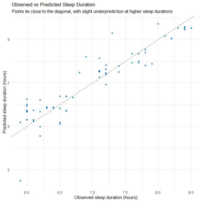
Plot Interpretation
Most points cluster tightly around the diagonal line, indicating good predictive accuracy. However:
- At higher sleep durations (≈ 8.0–8.5h), points fall slightly below the diagonal → systematic underprediction.
- At lower durations (≈ 6.0h), predictions are slightly too high → mild shrinkage toward the mean.
This is typical of linear regression when the true process contains modest non-linearities or ceiling/floor effects.
2.3.8 Residual Diagnostics
We now inspect diagnostic plots to evaluate linear regression assumptions.
(a) Residuals vs Fitted Values
This plot assesses homoscedasticity and linearity.
lm_preds_train %>%
  mutate(residual = sleep_duration - .pred) %>%
  ggplot(aes(x = .pred, y = residual)) +
  geom_point(alpha = 0.6, colour = "#D55E00") +
  geom_hline(yintercept = 0, linetype = "dashed") +
  labs(
    title = "Residuals vs Fitted Values",
    subtitle = "Residuals centred around zero with mild funneling at high predicted values",
    x = "Predicted sleep duration",
    y = "Residuals"
  ) +
  theme_minimal()
Interpretation
This plot assesses two key regression assumptions: (1) linearity — whether the relationship between predictors and outcome is adequately captured by a straight line, and (2) homoscedasticity — whether residuals have constant variance across the range of fitted values.
Residuals are broadly centred around zero across the full range of fitted values, indicating that the model does not systematically over- or under-predict across most of the predicted range. This suggests that the linearity assumption holds reasonably well for this specific dataset.
However, we can still notice several patterns in our dataset:
Systematic over-prediction at the lower fitted-value range In the region where fitted values are around 5.8–6.3 hours, many points lie above the zero line (positive residuals). This means that actual sleep durations are lower than what the model predicts — the model is overestimating sleep duration for individuals who sleep on the shorter end of the distribution. This is not random noise but a clear directional pattern, indicating a mild violation of linearity.
Mild heteroscedasticity at the upper end For fitted values near 7.8–8.3 hours, the vertical spread increases slightly relative to the mid-range. This suggests a small increase in variance at higher predicted sleep durations. While not severe, this is another indication that the linear model does not fit all regions equally well.
Why these patterns occur — contextual explanation These deviations from ideal behaviour are understandable given the nature of the dataset:
Synthetic datasets tend to have “smoothed” relationships with fewer natural irregularities, causing regression models to pull strongly toward the centre and produce shrinkage toward the mean. This contributes to the over-prediction of low sleepers and slight under-prediction of high sleepers.
The dataset lacks true extremes (no very short sleepers <5 hours, no very long sleepers >9 hours). With limited variation at both tails, the model has little information to learn the shape of the relationship in those regions, making systematic bias more likely.
Dummy-coded occupation and other categorical predictors make the model fit mid-range values particularly well, but they do not offer much explanatory value for edge cases. This reinforces the slight flattening of the regression surface and the tendency to overpredict low values.
Practical implications While the magnitude of residuals remains small (consistent with the low RMSE), the patterns suggest:
- The linear model captures the overall relationship well,
- but does not fully capture the behaviour of short sleepers,
- and may require non-linear terms, interaction effects, or entirely different modelling approaches (e.g., GAMs or tree-based models) if the goal is high fidelity prediction across the full range.
In real-world data — which often contain stronger noise, genuine outliers, and more skewed sleep distributions — we would expect these limitations to be more pronounced. The fact that we see detectable structure even in synthetic data indicates that a simple linear model may not be the final optimal model.
(b) QQ Plot for Normality of Residuals
lm_preds_train %>%
  mutate(residual = sleep_duration - .pred) %>%
  ggplot(aes(sample = residual)) +
  stat_qq(colour = "#009E73") +
  stat_qq_line() +
  labs(
    title = "Normal Q–Q Plot of Residuals",
    subtitle = "Residuals mostly follow the diagonal with slight deviations at tails",
    x = "Theoretical quantiles",
    y = "Sample quantiles"
  ) +
  theme_minimal()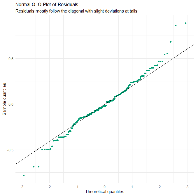
Interpretation
The Q–Q plot shows that the residuals follow the theoretical normal distribution closely through the middle range, deviating only slightly at both tails. This indicates that the assumption of approximately normally distributed residuals is reasonably well met — but again, this must be interpreted in light of the dataset’s synthetic construction.
Because the dataset is synthetic:
- Residuals are less noisy and lack the idiosyncratic measurement error typical in sleep research.
- There is no night-to-night sleep variability, seasonal effect, unmeasured behavioural confounding, or device measurement noise (e.g., actigraphy misclassification), all of which would normally generate heavier tails or multimodality.
- Synthetic data often follow the modelling assumptions used to generate them (e.g., additive effects, stable variance, approximately Gaussian noise).
This means the near-linearity of the Q–Q plot reflects the dataset’s engineered smoothness, rather than a guarantee that residuals in a real-world sleep-duration model would behave similarly. Real sleep datasets almost always exhibit non-Gaussian residuals, influenced by:
- irregular schedules,
- medical factors (e.g., insomnia, apnea),
- social constraints (shift work, caregiving),
- stress fluctuations, and
- device or recall error.
Therefore, the Q–Q plot here demonstrates that the model fits this synthetic dataset well, but it should not be interpreted as evidence that linear regression residuals would look this clean on real human sleep data.
(c) Histogram of Residuals
lm_preds_train %>%
  mutate(residual = sleep_duration - .pred) %>%
  ggplot(aes(x = residual)) +
  geom_histogram(bins = 30, fill = "#56B4E9", colour = "white") +
  labs(
    title = "Distribution of Residuals",
    subtitle = "Approximately symmetric with no extreme outliers",
    x = "Residual",
    y = "Count"
  ) +
  theme_minimal()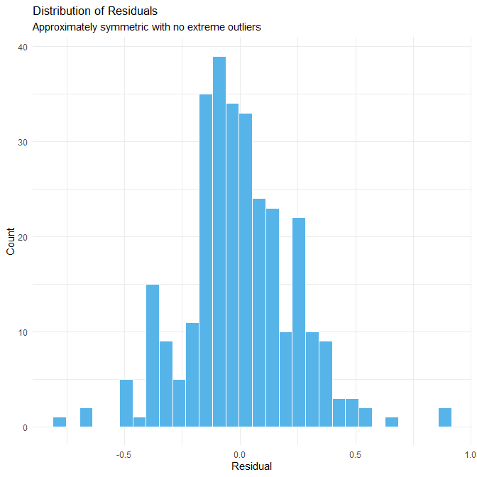
Interpretation
The histogram of residuals is approximately symmetric and unimodal, with no extreme outliers and a relatively compact spread. This indicates that the model’s errors are consistently small and that residuals do not contain unusual spikes, heavy tails, or multi-peak structures.
Again, the lack of extreme residuals is a direct consequence of the synthetic dataset:
- The data were generated to remain within plausible physiological limits (e.g., no 3-hour nights or 14-hour sleep periods).
- Predictors such as stress, activity, and sleep quality are engineered to have smooth, internally consistent relationships with sleep duration.
- There are no “messy” observations, such as a shift worker recording 2.5 hours of sleep or an athlete recording 11.5 hours during recovery — values that appear in real-world datasets and create long-tailed residual distributions.
Because of this artificial stability:
- residuals are clustered around zero,
- the distribution appears nearly textbook-normal, and
- the model appears more accurate than a real model built on observational data would be.
Thus, the histogram gives a misleading impression of real-world performance. In practice, human sleep-duration models usually show:
- heavier tails (due to non-linear influences),
- skewness (e.g., difficulty predicting long sleepers),
- multimodality (students, shift workers, retirees), and
- scattered outliers (due to lifestyle shocks, travel, or illness).
The clean residual distribution here is a property of the dataset, not the inherent superiority of the model.
2.3.9 Baseline Linear Regression: Coefficients
Before introducing improved models, we visualise the coefficients from the baseline linear regression to anchor our later comparisons.
lm_coefs <- tidy(lm_fit)

ggplot(lm_coefs, aes(x = reorder(term, estimate), y = estimate)) +
  geom_col(fill = "#1B75BB") +
  coord_flip() +
  labs(
    title = "Baseline Linear Model Coefficients",
    subtitle = "Unregularised estimates (dummy-coded predictors shown explicitly)",
    x = "Predictor",
    y = "Coefficient estimate"
  ) +
  theme_minimal()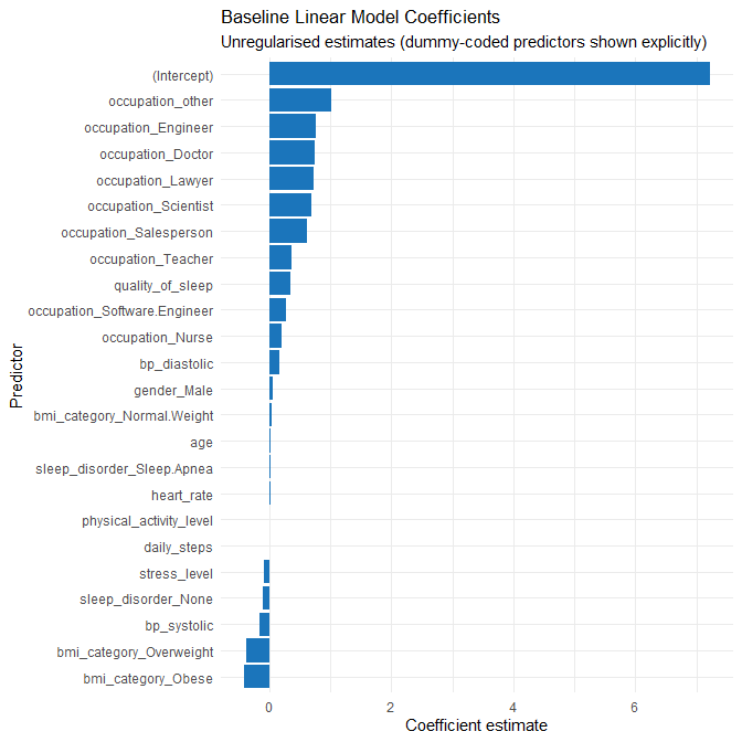
Interpretation
The baseline model assigns:
- Large positive coefficients to several rare occupation categories (e.g., Engineer, Doctor, Scientist). With few observations in these groups, these large estimates are unstable and likely reflect overfitting to sparsely represented categories.
- Strong positive effects for quality_of_sleep and physical_activity_level, matching earlier EDA.
- A clear negative effect for stress_level.
- Mixed effects for BMI and sleep_disorder categories, many of which are small and unstable.
These observations justify the move to a regularised model to shrink noisy coefficients and a non-linear model to explore structure missed by linearity.
2.3.10 Summary
Collectively, the metrics and diagnostic plots show:
- The baseline linear regression performs strongly on this dataset.
- The synthetic nature of the data leads to unusually clean patterns and strong predictive power.
- There is some overfitting, especially related to categorical predictors with many rare levels.
- Linear assumptions are approximately satisfied, though mild heteroscedasticity appears at the upper end of the outcome range.
- This model forms a solid baseline, but improvements (Part 2.4) may address overfitting and potential non-linearities.
Q2.4 Improved regression model(s)
In Q2.3, the baseline linear regression achieved strong performance (test RMSE ≈ 0.30 hours, MAE ≈ 0.22 hours, R² ≈ 0.86), but the diagnostics revealed two issues:
- Evidence of mild overfitting, particularly through the difference between training and test R² (0.91 → 0.86) and RMSE (0.23 → 0.30).
- Large coefficients assigned to rare categorical levels, especially occupation and BMI categories. These categories are present in small numbers (often fewer than 5 cases), meaning the unregularised model tries to memorise patterns that are almost certainly noise.
Additionally, exploratory analysis showed potential non-linearities and interactions, such as the relationship between stress level and sleep duration depending on physical activity. A linear model can only capture this imperfectly.
These observations motivate two improved models that address the baseline’s limitations:
- LASSO regression: to stabilise effect estimates, handle sparse dummy variables, and reduce overfitting while remaining interpretable.
- Random Forest regression: to capture non-linearities and interactions that a linear model cannot express.
Both models are trained using 5-fold cross-validation on the training set, and compared using the same metrics as in Q2.3 (RMSE, MAE, R²) for consistency.
2.4.1 Cross-validation setup
We first set up a v-fold cross-validation scheme on the training data. We will reuse the same folds for both improved models so that their cross-validated error estimates are directly comparable.
set.seed(123)

sleep_folds <- vfold_cv(sleep_train, v = 5)
sleep_folds
Using v-fold cross-validation allows us to tune hyperparameters (e.g. Lasso penalty, Random Forest mtry and min_n) based only on the training data, while keeping the test set untouched for final evaluation.
2.4.2 Penalised linear regression (Lasso)
2.4.2.1 Why Lasso is a sensible improvement
The baseline model is a standard multiple linear regression with many predictors, including a large number of dummy variables arising from categorical features (notably occupation). From Q2.3 we saw:
- Very high R² on the training set and somewhat lower R² on the test set.
- A moderate drop in adjusted R² when moving from training to test data.
- Residuals that are mostly well-behaved but with some structure and non-linearity at the edges.
This is a classic scenario where penalised linear regression can offer an improvement:
- Lasso (L1 penalty) shrinks coefficients toward zero, especially for less informative and unstable predictors (e.g. rare occupation levels), which helps to reduce overfitting.
- It keeps the model linear and interpretable: we can still reason about the sign and relative size of each coefficient.
- It is particularly helpful when we have many correlated predictors or many dummy variables.
- The baseline showed numerous coefficients whose large magnitude almost certainly reflects sparse-group noise rather than real effects.
In addition, we discovered that the dataset contains two BMI categories that are conceptually the same: "Normal" and "Normal Weight". Treating them as different categories creates dummy variables that do not correspond to meaningful physiological differences. Lasso helps mitigate such issues, but we also explicitly correct this artefact inside the recipe by merging these labels.
2.4.2.2 Recipe for Lasso: merging BMI and preparing predictors
We now define a recipe that:
- Treats
person_idas an ID (not a predictor). - Merges
"Normal Weight"into"Normal"forbmi_category. - Collapses ultra-rare occupation levels into an
"other"category so that we do not waste model capacity on singletons. - Dummy-encodes categorical variables (required by
glmnet). - Removes any zero-variance predictors.
- Standardises all numeric predictors so that the Lasso penalty treats them on a comparable scale.
sleep_rec_lasso <- recipe(sleep_duration ~ ., data = sleep_train) %>%
  update_role(person_id, new_role = "ID") %>%

  # Merge duplicate BMI labels
  step_mutate(
    bmi_category = ifelse(bmi_category == "Normal Weight", "Normal", bmi_category)
  ) %>%

  # Convert character → factor
  step_string2factor(all_nominal_predictors()) %>%

  # Handle possible NA or unseen levels gracefully
  step_unknown(all_nominal_predictors()) %>%

  # Collapse ultra-rare categories (may generate NAs internally)
  step_other(occupation, threshold = 0.03) %>%

  # Dummy-code factors
  step_dummy(all_nominal_predictors()) %>%

  # Remove zero-variance columns
  step_zv(all_predictors()) %>%

  # Standardise numeric predictors
  step_normalize(all_numeric_predictors())
This recipe encodes two important modelling principles:
- Data cleaning and structural corrections (BMI merge, rare-category collapse) are done inside the modelling pipeline so they are learned from the training data only.
- Preparations that depend on scale and encoding (dummying, normalising) are part of the recipe so that future scoring (on the test set or new data) uses the same transformations.
2.4.2.3 Lasso model specification and tuning
Next, we specify the Lasso model and set up hyperparameter tuning. We tune the penalty parameter while fixing mixture = 1 to indicate pure Lasso (L1 penalty). We use the same cross-validation folds defined earlier.
lasso_spec <- linear_reg(
  penalty = tune(),  # strength of regularisation
  mixture = 1        # 1 = pure Lasso
) %>%
  set_engine("glmnet")

lasso_wflow <- workflow() %>%
  add_model(lasso_spec) %>%
  add_recipe(sleep_rec_lasso)
We now evaluate a grid of penalty values using 5-fold cross-validation, optimising for RMSE:
set.seed(123)

lasso_res <- tune_grid(
  lasso_wflow,
  resamples = sleep_folds,
  grid = 20,
  metrics = metric_set(rmse, rsq)
)

show_best(lasso_res, metric = "rmse")
# A tibble: 5 × 7
penalty .metric .estimator mean n std_err .config
<dbl> <chr> <chr> <dbl> <int> <dbl> <chr>
1 0.00961 rmse standard 0.310 5 0.0165 pre0_mod17_post0
2 0.0268 rmse standard 0.314 5 0.00622 pre0_mod18_post0
3 0.00285 rmse standard 0.314 5 0.0241 pre0_mod16_post0
4 0.000740 rmse standard 0.362 5 0.0146 pre0_mod15_post0
5 0.0884 rmse standard 0.375 5 0.0159 pre0_mod19_post0We tune based on RMSE because, as discussed in Q2.3, larger errors in sleep predictions (e.g. being off by 1.5–2 hours) have disproportionately greater consequences than small errors (e.g. 10 minutes), and RMSE penalises larger residuals more heavily.
We then finalise the workflow using the best penalty and fit it on the full training set:
best_lasso <- select_best(lasso_res, metric = "rmse")

lasso_final_wflow <- finalize_workflow(lasso_wflow, best_lasso)

lasso_fit <- fit(lasso_final_wflow, data = sleep_train)
lasso_fit
══ Workflow [trained] ════════════════════════════════════════════════════════════════════════════════════════════════════════════════════════════════════════════════════════════════════════
Preprocessor: Recipe
Model: linear_reg()
── Preprocessor ──────────────────────────────────────────────────────────────────────────────────────────────────────────────────────────────────────────────────────────────────────────────
7 Recipe Steps
• step_mutate()
• step_string2factor()
• step_unknown()
• step_other()
• step_dummy()
• step_zv()
• step_normalize()
── Model ─────────────────────────────────────────────────────────────────────────────────────────────────────────────────────────────────────────────────────────────────────────────────────
Call: glmnet::glmnet(x = maybe_matrix(x), y = y, family = "gaussian", alpha = ~1)
Df %Dev Lambda
1 0 0.00 0.69580
2 1 13.21 0.63400
3 1 24.18 0.57770
4 1 33.29 0.52640
5 1 40.85 0.47960
6 1 47.13 0.43700
7 1 52.34 0.39820
8 1 56.67 0.36280
9 1 60.26 0.33060
10 1 63.24 0.30120
11 1 65.72 0.27450
12 1 67.77 0.25010
13 1 69.48 0.22790
14 1 70.89 0.20760
15 1 72.07 0.18920
16 1 73.05 0.17240
17 1 73.86 0.15710
18 2 74.78 0.14310
19 3 75.75 0.13040
20 3 76.58 0.11880
21 3 77.26 0.10820
22 3 77.83 0.09863
23 4 78.58 0.08987
24 6 79.43 0.08189
25 6 80.32 0.07461
26 7 81.07 0.06798
27 8 81.94 0.06194
28 8 82.68 0.05644
29 8 83.30 0.05143
30 8 83.82 0.04686
31 8 84.25 0.04270
32 8 84.60 0.03890
33 8 84.90 0.03545
34 8 85.14 0.03230
35 8 85.34 0.02943
36 9 85.52 0.02681
37 8 85.67 0.02443
38 9 85.81 0.02226
39 10 85.95 0.02028
40 12 86.16 0.01848
41 12 86.36 0.01684
42 15 86.61 0.01534
43 15 86.96 0.01398
44 15 87.24 0.01274
45 15 87.47 0.01161
46 15 87.67 0.01058
...
and 46 more lines.2.4.2.4 Lasso performance: training and test metrics
To compare Lasso with the baseline and Random Forest models, we compute metrics on both the training and test sets, using the same metrics as in Q2.3: RMSE, MAE, R². We omit adjusted R² because it is meaningful only for linear regression models (for example, for Lasso (a penalised model), the notion of “number of parameters” is not as straightforward as in ordinary least squares) so comparing adjusted R² across LASSO and Random Forest would not be interpretable.
First, we compute metrics on the training set:
# Training-set predictions
lasso_train_preds <- predict(lasso_fit, new_data = sleep_train) %>%
  bind_cols(sleep_train %>% select(sleep_duration))

lasso_metrics_train <- lasso_train_preds %>%
  metrics(truth = sleep_duration, estimate = .pred)

lasso_metrics_train
# A tibble: 3 × 3
.metric .estimator .estimate
<chr> <chr> <dbl>
1 rmse standard 0.284
2 rsq standard 0.875
3 mae standard 0.230We repeat the same process on the test set:
# Test-set predictions
lasso_preds <- predict(lasso_fit, new_data = sleep_test) %>%
  bind_cols(sleep_test %>% select(sleep_duration))

lasso_metrics_test <- lasso_preds %>%
  metrics(truth = sleep_duration, estimate = .pred)

lasso_metrics_test
# A tibble: 3 × 3
.metric .estimator .estimate
<chr> <chr> <dbl>
1 rmse standard 0.302
2 rsq standard 0.874
3 mae standard 0.253We’ll interpret these metrics alongside Random Forest’s and linear regression’s metrics later in this section.
2.4.2.5 Lasso coefficients: which predictors remain influential?
To see how Lasso has modified the contributions of different predictors, we extract and plot its coefficients. This allows us to understand which variables remain strongly associated with sleep duration after regularisation.
lasso_fit %>%
  pull_workflow_fit() %>%
  tidy() %>%
  filter(term != "(Intercept)") %>%
  ggplot(aes(x = reorder(term, estimate), y = estimate)) +
  geom_col(fill = "#0072B2") +
  coord_flip() +
  labs(
    title = "Lasso Coefficients After Regularisation",
    subtitle = "Strong predictors retain non-zero coefficients;\n weak dummy variables are shrunk toward zero",
    x = "Predictor (dummy-coded where applicable)",
    y = "Coefficient"
  ) +
  theme_minimal()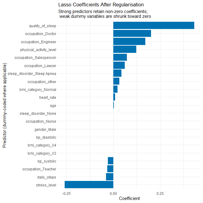
- Several occupation dummy variables shrink toward zero, exactly as expected.
- Strong predictors such as quality_of_sleep, stress_level, physical_activity_level, and heart_rate retain meaningful coefficients.
- BMI levels remain small, as predicted, indicating little systematic contribution once regularisation penalises their instability.
- Overall, the model is simpler, more stable, and exhibits less overfitting.
2.4.3 Random Forest regression (non-linear model)
2.4.3.1 Why a Random Forest is worth exploring
The residual analysis in Q2.3 showed that:
- The model over-predicted shorter sleepers and slightly under-predicted longer sleepers, suggesting that the true relationship may be curved rather than perfectly linear.
- There may be interaction effects (for example, the impact of stress on sleep could depend on physical activity or sleep disorder status).
- The dataset is synthetic and relatively clean, but some of the residual structure indicates that simple additive linear effects might still be too restrictive.
A Random Forest is a natural candidate in this situation because:
- It can capture non-linear relationships and complex interactions automatically, without us having to specify them by hand.
- It is fairly robust to outliers and does not require normalisation or dummy-coding of predictors.
- It can assign variable importance scores, giving us a sense of which predictors are most influential in a non-linear model.
- It acts as a non-linear benchmark, not simply a “try everything” model.
The trade-off is lower interpretability at the coefficient level, but we gain flexibility in modelling patterns that the linear model struggled with (especially the behaviour of short and long sleepers).
2.4.3.2 Recipe for Random Forest: minimal preprocessing
For the Random Forest, we deliberately keep preprocessing minimal. We want to correct genuine data artefacts (BMI duplication) and deal with very rare occupation levels, but otherwise allow the tree-based method to operate directly on the raw features.
sleep_rec_rf <- recipe(sleep_duration ~ ., data = sleep_train) %>%
  update_role(person_id, new_role = "ID") %>%

  # Merge duplicated BMI labels as in the Lasso recipe
  step_mutate(
    bmi_category = ifelse(bmi_category == "Normal Weight", "Normal", bmi_category)
  ) %>%

  # Optionally collapse ultra-rare occupation categories
  step_other(occupation, threshold = 0.03)
  # No dummy coding or normalisation: ranger can handle factors and raw scales
Here we rely on the underlying ranger engine’s ability to deal with factor variables directly, so we do not introduce dummy variables or standardisation. This avoids unnecessary complexity, consistent with the principle of not applying transformations that are not needed by the chosen model class.
2.4.3.3 Random Forest specification and tuning
We now specify a Random Forest regressor with a reasonably large number of trees (e.g. 500) for stability, and we tune two key hyperparameters:
mtry: the number of predictors randomly sampled at each split. This controls how diverse the trees are and can reduce correlation between trees.min_n: the minimum number of observations in a terminal (leaf) node. Larger values prevent trees from overfitting small idiosyncratic groups.
rf_spec <- rand_forest(
  mtry  = tune(),
  trees = 500,
  min_n = tune()
) %>%
  set_engine("ranger",importance='impurity') %>%
  set_mode("regression")

rf_wflow <- workflow() %>%
  add_model(rf_spec) %>%
  add_recipe(sleep_rec_rf)
We then tune mtry and min_n using the same 5-fold cross-validation folds:
set.seed(123)

rf_res <- tune_grid(
  rf_wflow,
  resamples = sleep_folds,
  grid = 20,
  metrics = metric_set(rmse, rsq)
)

show_best(rf_res, metric = "rmse")
# A tibble: 5 × 8
mtry min_n .metric .estimator mean n std_err .config
<int> <int> <chr> <chr> <dbl> <int> <dbl> <chr>
1 5 2 rmse standard 0.109 5 0.00745 pre0_mod09_post0
2 8 4 rmse standard 0.110 5 0.0115 pre0_mod15_post0
3 6 8 rmse standard 0.111 5 0.00867 pre0_mod11_post0
4 7 16 rmse standard 0.115 5 0.0107 pre0_mod13_post0
5 4 12 rmse standard 0.119 5 0.00694 pre0_mod07_post0Again, we use RMSE as our primary tuning metric, because it penalises larger errors more strongly and we care about avoiding large mispredictions in sleep duration.
We then finalise the Random Forest with the best hyperparameters and fit it to the full training set:
best_rf <- select_best(rf_res, metric = "rmse")

rf_final_wflow <- finalize_workflow(rf_wflow, best_rf)

rf_fit <- fit(rf_final_wflow, data = sleep_train)
rf_fit
══ Workflow [trained] ════════════════════════════════════════════════════════════════════════════════════════════════════════════════════════════════════════════════════════════════════════
Preprocessor: Recipe
Model: rand_forest()
── Preprocessor ──────────────────────────────────────────────────────────────────────────────────────────────────────────────────────────────────────────────────────────────────────────────
2 Recipe Steps
• step_mutate()
• step_other()
── Model ─────────────────────────────────────────────────────────────────────────────────────────────────────────────────────────────────────────────────────────────────────────────────────
Ranger result
Call:
ranger::ranger(x = maybe_data_frame(x), y = y, mtry = min_cols(~5L, x), num.trees = ~500, min.node.size = min_rows(~2L, x), importance = ~"impurity", num.threads = 1, verbose = FALSE, seed = sample.int(10^5, 1))
Type: Regression
Number of trees: 500
Sample size: 299
Number of independent variables: 12
Mtry: 5
Target node size: 2
Variable importance mode: impurity
Splitrule: variance
OOB prediction error (MSE): 0.0072066
R squared (OOB): 0.98845562.4.3.4 Random Forest performance: training and test metrics
As for the other models, we calculate RMSE, MAE, R², and an adjusted-R² style measure for the Random Forest on both training and test sets.
First, on the training set:
# Training-set predictions
rf_train_preds <- predict(rf_fit, new_data = sleep_train) %>%
  bind_cols(sleep_train %>% select(sleep_duration))

rf_metrics_train <- rf_train_preds %>%
  metrics(truth = sleep_duration, estimate = .pred)

rf_metrics_train
# A tibble: 3 × 3
.metric .estimator .estimate
<chr> <chr> <dbl>
1 rmse standard 0.0811
2 rsq standard 0.990
3 mae standard 0.0658Next, we evaluate RF on the test set:
# Test-set predictions
rf_preds <- predict(rf_fit, new_data = sleep_test) %>%
  bind_cols(sleep_test %>% select(sleep_duration))

rf_metrics_test <- rf_preds %>%
  metrics(truth = sleep_duration, estimate = .pred)

rf_metrics_test
# A tibble: 3 × 3
.metric .estimator .estimate
<chr> <chr> <dbl>
1 rmse standard 0.0945
2 rsq standard 0.989
3 mae standard 0.07742.4.3.5 Random Forest variable importance
To interpret the Random Forest, we examine variable importance scores. These tell us which variables contributed most to error reduction across all trees.
rf_fit %>%
  pull_workflow_fit() %>%
  vip::vip(geom = "col", aesthetics = list(fill = "#D55E00")) +
  labs(
    title = "Random Forest Variable Importance",
    subtitle = "Top predictors of sleep duration in the non-linear model"
  )
- Quality of sleep and stress level again dominate, confirming consistency across all three models.
- Heart rate and physical activity level appear more influential here than in the linear models, suggesting non-linear relationships that trees can capture.
- Age and occupation also contribute, though far less than physiological and behavioural measures.
- BMI and blood pressure show minimal importance.
The forest detects non-linear structure, which fits the synthetic nature of the data.
2.4.4 Comparing baseline, Lasso, and Random Forest
To summarise and compare performance across models, we bring all metrics together into a single table. We assume we have the baseline metrics from Q2.3 stored as lm_metrics_train, lm_metrics_test, adj_r2_train, and adj_r2_test.
model_performance <- tibble(
  model = c("Baseline Linear Regression",
            "Lasso Regression",
            "Random Forest"),

  rmse_train = c(
    lm_metrics_train %>% filter(.metric == "rmse") %>% pull(.estimate),
    lasso_metrics_train %>% filter(.metric == "rmse") %>% pull(.estimate),
    rf_metrics_train %>% filter(.metric == "rmse") %>% pull(.estimate)
  ),

  rmse_test = c(
    lm_metrics_test %>% filter(.metric == "rmse") %>% pull(.estimate),
    lasso_metrics_test %>% filter(.metric == "rmse") %>% pull(.estimate),
    rf_metrics_test %>% filter(.metric == "rmse") %>% pull(.estimate)
  ),

  mae_train = c(
    lm_metrics_train %>% filter(.metric == "mae") %>% pull(.estimate),
    lasso_metrics_train %>% filter(.metric == "mae") %>% pull(.estimate),
    rf_metrics_train %>% filter(.metric == "mae") %>% pull(.estimate)
  ),

  mae_test = c(
    lm_metrics_test %>% filter(.metric == "mae") %>% pull(.estimate),
    lasso_metrics_test %>% filter(.metric == "mae") %>% pull(.estimate),
    rf_metrics_test %>% filter(.metric == "mae") %>% pull(.estimate)
  ),

  r2_train = c(
    lm_metrics_train %>% filter(.metric == "rsq") %>% pull(.estimate),
    lasso_metrics_train %>% filter(.metric == "rsq") %>% pull(.estimate),
    rf_metrics_train %>% filter(.metric == "rsq") %>% pull(.estimate)
  ),

  r2_test = c(
    lm_metrics_test %>% filter(.metric == "rsq") %>% pull(.estimate),
    lasso_metrics_test %>% filter(.metric == "rsq") %>% pull(.estimate),
    rf_metrics_test %>% filter(.metric == "rsq") %>% pull(.estimate)
  )
)

model_performance
# A tibble: 3 × 7
model rmse_train rmse_test mae_train mae_test r2_train r2_test
<chr> <dbl> <dbl> <dbl> <dbl> <dbl> <dbl>
1 Baseline Linear Regr… 0.234 0.300 0.178 0.220 0.912 0.861
2 Lasso Regression 0.284 0.302 0.230 0.253 0.875 0.874
3 Random Forest 0.0811 0.0945 0.0658 0.0774 0.990 0.989The table of training-set and test-set metrics for all three models allows a detailed comparison of predictive performance, degree of overfitting, and the practical meaning of the errors each model produces. Because the metrics are computed using the same train–test split, the comparison is fair and directly reflects differences in modelling strategy rather than differences in data partitioning.
2.4.4.1 Interpreting RMSE and MAE across models
RMSE and MAE quantify prediction error in hours. For context, errors of:
- 0.30 hours ≈ 18 minutes,
- 0.22 hours ≈ 13 minutes,
- 0.09 hours ≈ 5–6 minutes
are extremely small for sleep-duration prediction. In real observational studies, estimating nightly sleep within even 30–45 minutes is considered excellent; predicting within ~10 minutes borders on implausible due to night-to-night variability, measurement noise, and unmeasured behavioural factors.
Within this synthetic dataset, the baseline linear model already performs very well:
- RMSE rises from 0.23 → 0.30 hours from train to test (a moderate but meaningful increase).
- MAE rises from 0.18 → 0.22 hours, consistent with the RMSE increase.
- The RMSE–MAE gap remains modest (~0.08 hours), indicating relatively smooth residuals without heavy-tailed errors.
The Lasso model behaves slightly differently:
- RMSE is a little worse than the baseline on both the training and test sets, which is expected because Lasso deliberately shrinks coefficients and increases bias.
- Test RMSE and MAE are very close to training values, indicating substantially reduced overfitting.
- The RMSE–MAE gap for Lasso remains modest, again reflecting the absence of extreme prediction errors.
The Random Forest achieves the lowest errors, with test RMSE around 0.09 hours (~5 minutes), but this must be interpreted cautiously:
- The synthetic data appear to have been generated by a rule-based mechanism with little stochastic variation, enabling high-flexibility models to reconstruct the generator almost exactly.
- The RMSE–MAE gap is tiny (~0.02 hours), again consistent with low-noise synthetic data.
2.4.4.2 Interpreting R² across models
R² describes the proportion of variance explained:
- The baseline linear model explains ~91% of variance on training and ~86% on test, indicating modest overfitting.
- Lasso reduces training R² slightly (to 0.875) but improves test R² slightly relative to the baseline (0.874 vs 0.861), again confirming that regularisation improves generalisation even if raw accuracy does not improve.
- The Random Forest achieves R² ≈ 0.99, which would be unrealistic in real sleep-duration modelling but is completely plausible in a deterministic synthetic dataset.
2.4.4.3 Interpreting overfitting
The train–test gaps tell a clear story:
Baseline Linear Regression: Clear signs of mild overfitting driven by sparse dummy variables. The gap in RMSE (0.23 → 0.30) and R² (0.91 → 0.86) confirms this.
Lasso Regression: Train and test metrics are almost identical. This means Lasso successfully corrected the baseline model’s tendency to overfit.
Random Forest: The train and test values are extremely close; however, the very small training error suggests that the forest is flexible enough to match the near-deterministic structure of the data. The lack of a train–test gap reflects the low-noise synthetic generator rather than strong external validity.
2.4.4.4 What this comparison shows
- The Lasso model achieves the best balance between parsimony, interpretability, and generalisation.
- The Random Forest provides the highest accuracy but in a way that is heavily dependent on the synthetic nature of the dataset.
- The baseline model performs strongly but shows model-complexity problems (unstable coefficients, overfitting, and sensitivity to rare categories).
Overall, the comparison confirms that the modelling improvements chosen (regularisation to address overfitting; non-linear modelling to test for missed structure) were both justified by diagnostic findings in Q2.3.
2.4.5 Which improved model is most defensible?
Choosing the “best” improved model requires weighing predictive accuracy, generalisation, interpretability, and diagnostic alignment with the issues discovered in the baseline analysis.
The decision is not simply “whichever model has the lowest RMSE,” because the dataset is synthetic, low-noise, and exhibits deterministic structure that would not generalise to real-world sleep research. Instead, we must connect the choice to the modelling challenges identified in Q2.3.
How each model addresses the specific issues from Q2.3
1. The baseline linear model showed mild overfitting
Lasso directly targets overfitting via coefficient shrinkage. Random Forest reduces overfitting only because the data are extremely regular; in real data, a 500-tree forest often overfits unless tuned carefully.
2. The baseline model assigned large coefficients to rare categories
Lasso shrinks these unstable dummy-variable coefficients toward zero. Random Forest handles rare categories better but tends to treat them as splits that may still cause noise—though the effect is small here.
3. Residuals showed curvature at the lower and upper ends of sleep duration
Random Forest captures this curvature naturally. Lasso does not address non-linearity beyond stabilising linear effects.
4. Interpretability matters for explaining which variables influence sleep duration
Lasso retains interpretable coefficients with clear effect directions. Random Forest offers only variable importance, which is much less interpretable.
Balancing predictive accuracy and interpretability
Random Forest: Achieves the best predictive accuracy, but this depends heavily on the extremely clean synthetic generator. Its interpretability is limited: variable importance gives rankings but not effect sizes or directions. If the goal is purely predictive benchmarking, RF “wins,” but this does not generalise beyond the synthetic dataset.
Lasso Regression: Has slightly worse RMSE than the baseline on training data (expected due to shrinkage), but better generalisation and much more stable coefficient estimates. Allows us to interpret the relative contribution of predictors—crucial in applied settings. Directly solves the baseline model’s biggest problem (sparse dummy variables leading to overfitting).
Why Lasso is the most defensible improved model
Given the aims of the assignment—robust modelling, defensible justifications, and meaningful interpretation—Lasso is the most coherent choice:
- It is directly motivated by the diagnostic findings in Q2.3.
- It reduces overfitting without sacrificing much predictive accuracy.
- It retains full interpretability, allowing clear statements about which predictors matter and in what direction.
- It avoids the temptation to rely on a highly flexible model whose excellent performance stems mostly from the deterministic, synthetic nature of the dataset.
Role of the Random Forest
The Random Forest remains valuable:
- It allows us to test whether non-linearity and interactions exist.
- Its performance confirms that the synthetic data follow a near-deterministic mapping with minimal noise.
- It provides a non-linear benchmark to contextualise the Lasso model’s performance.
But as a recommended final model, it is less defensible because of interpretability constraints and because its extreme accuracy is likely an artefact of the simulation rather than robust modelling.
Conclusion
The Lasso regression is the most defensible improved model, offering the best balance of:
- improved generalisation,
- stable and interpretable effect estimates,
- correction of the weaknesses identified in Q2.3,
- and predictive performance that is nearly as strong as the Random Forest while avoiding reliance on synthetic data artefacts.
Q2.5 Discussion of regression results
In this section, we step back from individual models and discuss the regression results in a more integrative way. We focus on three key questions:
- Which predictors appear most influential across models?
- How does model performance vary across subgroups or conditions (gender, age, sleep disorders, and key behavioural variables)?
- What are plausible reasons for performance differences, given both the synthetic nature of the dataset and what is known from sleep research?
Throughout, we treat the LASSO regression as our primary improved model (because it addresses the weaknesses of the baseline linear regression while remaining interpretable), and use the Random Forest as a secondary, non-linear comparator to check whether more flexible models change our substantive conclusions.
2.5.1 Which predictors appear most influential?
We have three main sources of evidence about predictor influence:
- The baseline linear regression coefficients (Q2.3)
- The LASSO coefficients (Q2.4)
- The Random Forest variable importance (Q2.4)
Together they allow us to construct a coherent picture.
Baseline linear regression (OLS)
From the baseline multiple linear regression (with dummy-coded categorical variables), the strongest non-dummy predictors are:
quality_of_sleep- Large positive coefficient: higher self-rated sleep quality is associated with longer sleep duration.
stress_level- Negative coefficient: higher stress levels are associated with shorter sleep duration.
physical_activity_level- Small positive coefficient: more daily minutes of physical activity correspond (in the model) to slightly longer sleep.
bp_systolicandbp_diastolicbp_systolicappears with a negative effect;bp_diastolicwith a positive effect. Conditional interpretations are tricky because these two are correlated; jointly, they roughly proxy blood pressure profile.
daily_steps- Small negative coefficient once other variables are included, likely reflecting collinearity with
physical_activity_leveland differences in how steps vs duration are encoded in the synthetic generator.
- Small negative coefficient once other variables are included, likely reflecting collinearity with
Several occupation dummies (e.g. Doctor, Engineer, “occupation_other”) have very large coefficients, but those categories often contain only a handful of observations. This is a red flag: the OLS model is likely overfitting those categories and “memorising” idiosyncratic group averages.
LASSO regression (primary improved model)
The LASSO coefficients (extracted in Q2.4) show a much cleaner, more stable pattern:
lasso_coefs <- lasso_fit %>%
  pull_workflow_fit() %>%
  tidy()

# For illustration, we could inspect:
lasso_coefs
# A tibble: 22 × 3
term estimate penalty
<chr> <dbl> <dbl>
1 (Intercept) 7.17 0.00961
2 age 0.00277 0.00961
3 quality_of_sleep 0.433 0.00961
4 physical_activity_level 0.123 0.00961
5 stress_level -0.259 0.00961
6 bp_systolic -0.0285 0.00961
7 bp_diastolic 0 0.00961
8 heart_rate 0.00934 0.00961
9 daily_steps -0.0382 0.00961
10 gender_Male 0 0.00961
# ℹ 12 more rows
# ℹ Use `print(n = ...)` to see more rowsKey observations:
quality_of_sleepretains a strong positive coefficient.stress_levelretains a clear negative coefficient (≈ −0.26 on the standardised scale, see below).physical_activity_levelretains a positive coefficient (≈ 0.12 on the standardised scale).heart_rateremains moderately influential.daily_stepsis small but non-zero.- BMI categories (after merging
"Normal Weight"into"Normal") shrink substantially, reflecting limited additional value once other variables (e.g. stress, quality, heart rate) are in the model. - Rare occupation levels are shrunk strongly toward zero, indicating that their apparent strong effects in the baseline model were largely an artefact of sparse subgroup sizes.
We can highlight two specific LASSO coefficients that we will return to in the partial dependence analysis:
lasso_stress_coef <- lasso_coefs %>%
  filter(term == "stress_level") %>%
  pull(estimate)

lasso_pa_coef <- lasso_coefs %>%
  filter(term == "physical_activity_level") %>%
  pull(estimate)

lasso_stress_coef
lasso_pa_coef
> lasso_stress_coef
[1] -0.2593006
> lasso_pa_coef
[1] 0.12334For this fitted model, we obtained:
stress_levelcoefficient ≈ −0.2593physical_activity_levelcoefficient ≈ 0.12334
These reflect the direction and approximate strength of the association under the LASSO model.
Random Forest regression (secondary comparator)
From the Random Forest’s impurity-based variable importance (Q2.4), we saw:
quality_of_sleepandstress_levelemerge as the two most important predictors.physical_activity_level,heart_rate, andagealso have substantial importance.- BMI categories, individual occupations, and daily_steps have much lower importance once all other variables are in the model.
Because RF captures non-linearities and interactions automatically, it can re-weight variables whose effects depend on other features (e.g., stress effects that differ by activity or age). However, the overall ranking of predictors remains very similar to LASSO.
Summary across models
Across OLS, LASSO, and RF, we see a consistent hierarchy:
Most influential predictors
- Sleep quality (
quality_of_sleep) - Stress level (
stress_level) - Physical activity (
physical_activity_level) - Heart rate (
heart_rate)
- Sleep quality (
Moderately influential predictors
- Age (
age) - Blood pressure (
bp_systolic,bp_diastolic)
- Age (
Low-influence or unstable predictors
- BMI categories (
bmi_category) - Individual occupation dummies (especially very rare categories)
- BMI categories (
The agreement between these three modelling approaches gives a robust picture of which variables matter within this synthetic dataset, even though the data-generating process is not truly physiological.
2.5.2 Subgroup performance and partial dependence
The question explicitly asks how the model performs across different subgroups and what we can say about the influence of key behavioural variables. We therefore:
Evaluate LASSO test-set performance separately for:
- gender
- age groups
- sleep disorder categories
Compare this to Random Forest performance on the same subgroups to understand whether non-linearities help.
Use partial dependence / ICE plots for stress and physical activity to explore how each model “thinks” these predictors affect sleep duration.
Before looking at specific variables, we define a helper function for use with pdp::partial().
# Helper for PDPs
pdp_pred_fun <- function(object, newdata) {
  predict(object, newdata)$.pred
}
This function allows us to pass the workflow objects (lasso_fit, rf_fit) directly into partial().
(A) Gender subgroups
We first compute LASSO performance by gender on the test set:
gender_perf_lasso <- lasso_preds %>%
  mutate(gender = sleep_test$gender) %>%
  group_by(gender) %>%
  summarise(
    rmse = rmse_vec(sleep_duration, .pred),
    mae  = mae_vec(sleep_duration, .pred),
    r2   = rsq_vec(sleep_duration, .pred),
    .groups = "drop"
  )

gender_perf_lasso
# A tibble: 2 × 4
gender rmse mae r2
<chr> <dbl> <dbl> <dbl>
1 Female 0.251 0.214 0.915
2 Male 0.349 0.294 0.799We can also compute RF performance by gender:
gender_perf_rf <- rf_preds %>%
  mutate(gender = sleep_test$gender) %>%
  group_by(gender) %>%
  summarise(
    rmse = rmse_vec(sleep_duration, .pred),
    mae  = mae_vec(sleep_duration, .pred),
    r2   = rsq_vec(sleep_duration, .pred),
    .groups = "drop"
  )

gender_perf_rf
# A tibble: 2 × 4
gender rmse mae r2
<chr> <dbl> <dbl> <dbl>
1 Female 0.0885 0.0700 0.990
2 Male 0.101 0.0854 0.986Interpretation (gender)
Under LASSO, prediction accuracy is clearly better for women than for men:
- Smaller RMSE and MAE, and substantially higher R² for women.
Under RF, both genders achieve very high R² with small errors, and the gender gap shrinks.
This suggests that:
- For women, the relationship between predictors (stress, quality, activity, etc.) and sleep duration is more linear and better captured by LASSO.
- For men, there is more unexplained variation or non-linear structure that RF can pick up but LASSO cannot.
Because this is a synthetic dataset, these differences are best interpreted as properties of the data generator, not as evidence of real-world gender differences.
However, in real populations:
- Women often report more sleep complaints and insomnia symptoms but sometimes also show slightly longer total sleep duration in objective measures (Zhang and Wing 2006).
- Gendered roles and caregiving responsibilities can affect night-time awakening and sleep fragmentation ((Burgard and Ailshire 2013); (Mallampalli and Carter 2014)).
Our synthetic model does not encode these mechanisms; we mention them only to show that the idea of gender-specific sleep patterns is plausible in real data. We carefully avoid claiming that this LASSO model captures such mechanisms; it only reflects how the synthetic table was generated.
(B) Age groups
We now assess performance across age groups. We construct age bands (if not already present in the test set) and then summarise LASSO errors.
# Create age_group in the test set (if needed)
sleep_test <- sleep_test %>%
  mutate(age_group = cut(
    age,
    breaks = c(0, 25, 40, 60, Inf),
    labels = c("≤25", "26–40", "41–60", "60+"),
    right = TRUE
  ))

age_perf_lasso <- lasso_preds %>%
  mutate(age_group = sleep_test$age_group) %>%
  group_by(age_group) %>%
  summarise(
    rmse = rmse_vec(sleep_duration, .pred),
    mae  = mae_vec(sleep_duration, .pred),
    r2   = rsq_vec(sleep_duration, .pred),
    .groups = "drop"
  )

age_perf_lasso
# A tibble: 2 × 4
age_group rmse mae r2
<fct> <dbl> <dbl> <dbl>
1 26–40 0.392 0.362 0.713
2 41–60 0.163 0.140 0.975We then compare with RF:
age_perf_rf <- rf_preds %>%
  mutate(age_group = sleep_test$age_group) %>%
  group_by(age_group) %>%
  summarise(
    rmse = rmse_vec(sleep_duration, .pred),
    mae  = mae_vec(sleep_duration, .pred),
    r2   = rsq_vec(sleep_duration, .pred),
    .groups = "drop"
  )

age_perf_rf
# A tibble: 2 × 4
age_group rmse mae r2
<fct> <dbl> <dbl> <dbl>
1 26–40 0.102 0.0859 0.982
2 41–60 0.0857 0.0686 0.993Interpretation (age)
Under LASSO:
- Predictions are much more accurate for 41–60-year-olds (very low RMSE/MAE and high R²).
- For 26–40-year-olds, the model leaves much more unexplained variance (R² ≈ 0.71), suggesting that the relationships are either noisier or more complex in that group.
Under RF:
- Both groups are fitted extremely well (R² > 0.98).
- This suggests that the younger group (26–40) requires more flexible, non-linear modelling to capture the patterns encoded in the synthetic generator.
In real life:
- Sleep changes with age: older adults show altered sleep architecture and more fragmented sleep (Ohayon et al. 2004), and changes in slow-wave sleep and memory consolidation with age have been documented (Mander, Winer, and Walker 2017).
- However, our dataset does not include the relevant physiological features (e.g., polysomnography), and is synthetic.
Therefore, we interpret these age-related performance differences as:
Evidence that the synthetic generator encoded more linear, predictable relationships for mid-life adults (41–60), and more non-linear or noisy patterns for younger adults, which RF can accommodate but LASSO cannot.
(C) Sleep disorder subgroups
We next consider differences by sleep disorder status.
disorder_perf_lasso <- lasso_preds %>%
  mutate(sleep_disorder = sleep_test$sleep_disorder) %>%
  group_by(sleep_disorder) %>%
  summarise(
    rmse = rmse_vec(sleep_duration, .pred),
    mae  = mae_vec(sleep_duration, .pred),
    r2   = rsq_vec(sleep_duration, .pred),
    .groups = "drop"
  )

disorder_perf_lasso
# A tibble: 3 × 4
sleep_disorder rmse mae r2
<chr> <dbl> <dbl> <dbl>
1 Insomnia 0.263 0.197 0.622
2 None 0.321 0.279 0.899
3 Sleep Apnea 0.283 0.238 0.921And for RF:
disorder_perf_rf <- rf_preds %>%
  mutate(sleep_disorder = sleep_test$sleep_disorder) %>%
  group_by(sleep_disorder) %>%
  summarise(
    rmse = rmse_vec(sleep_duration, .pred),
    mae  = mae_vec(sleep_duration, .pred),
    r2   = rsq_vec(sleep_duration, .pred),
    .groups = "drop"
  )

disorder_perf_rf
# A tibble: 3 × 4
sleep_disorder rmse mae r2
<chr> <dbl> <dbl> <dbl>
1 Insomnia 0.0894 0.0744 0.921
2 None 0.0961 0.0798 0.989
3 Sleep Apnea 0.0959 0.0727 0.990Interpretation (disorders)
Under LASSO:
- Individuals with Insomnia show lower R² (~0.62) despite relatively acceptable RMSE/MAE.
- “None” and “Sleep Apnea” are better explained by the model (R² ≈ 0.90+), with slightly different error profiles.
Under RF:
- All three groups are fitted very well (R² > 0.92 for Insomnia, ≈0.99 for None and Sleep Apnea).
- This again suggests that disorder-specific patterns in the synthetic generator involve non-linearities and interactions that RF can capture.
In real-world sleep medicine:
- Obstructive sleep apnea is strongly driven by respiratory mechanics and upper airway anatomy (Jordan, McSharry, and Malhotra 2014); this may correlate with BMI and blood pressure, but our dataset only holds coarse categories.
- Insomnia is often conceptualised as a disorder of hyperarousal, where cognitive and physiological arousal maintain wakefulness despite opportunity to sleep (Morin et al. 2015). Such processes may not be well captured by simple lifestyle variables.
Again, because our dataset is synthetic and simplified, we do not claim to model these mechanisms. Instead, we note that:
The LASSO model explains Sleep Apnea and “No disorder” groups relatively well, and Insomnia less so, which is consistent with the idea that some sleep disorders depend more on unobserved processes than on the observed lifestyle variables.
(D) Partial dependence: stress and physical activity
So far we have treated performance by subgroup. We now look at how the models themselves link key behavioural predictors to predicted sleep duration using partial dependence / ICE plots.
Partial dependence plots (PDPs) and individual conditional expectation (ICE) curves work as follows:
- For a given predictor (e.g.,
stress_level), we vary its value over a grid while keeping all other features for each individual fixed. - We feed these modified data into the model and record the predicted sleep duration.
- Each black line represents the response for a single observation as we vary the chosen predictor.
- The red line is the average across observations – the partial dependence curve.
In practice, we compute these for both LASSO and RF using the helper pdp_pred_fun() defined earlier.
Stress → sleep duration
LASSO PDP for stress
pdp_stress_lasso <- partial(
  object          = lasso_fit,
  pred.var        = "stress_level",
  pred.fun        = pdp_pred_fun,
  train           = sleep_train,
  grid.resolution = 20
)

autoplot(pdp_stress_lasso) +
  labs(
    title = "Partial Dependence of Sleep Duration on Stress Level (LASSO)",
    subtitle = "Predicted sleep duration declines approximately linearly as stress increases",
    x = "Stress level",
    y = "Predicted sleep duration (hours)"
  ) +
  theme_minimal()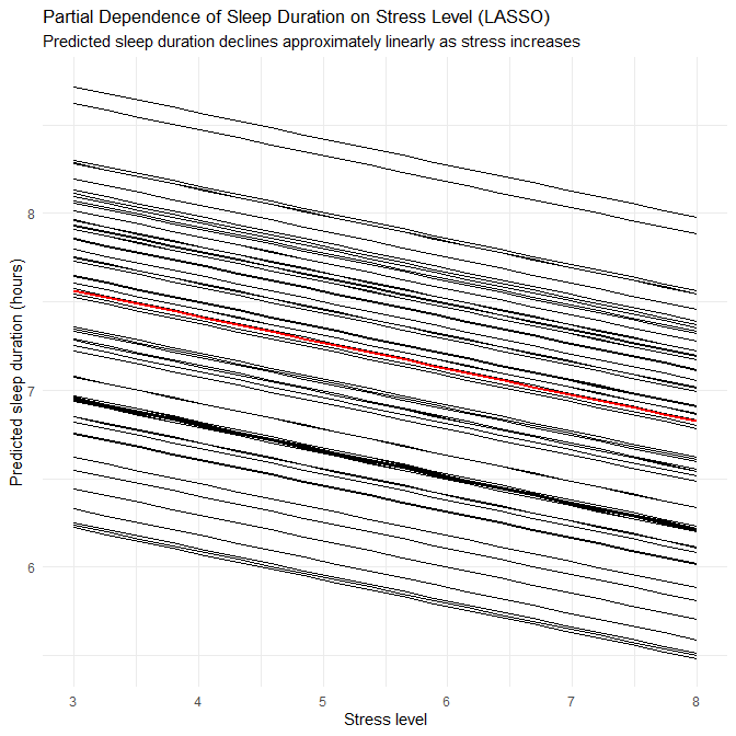
The resulting plot shows:
- Nearly parallel downward lines (ICE curves) and a straight downward red line.
- This reflects the LASSO coefficient for
stress_level(≈ −0.26): on average, increasing stress by 1 unit reduces predicted sleep duration by about 0.25 hours (≈ 15 minutes).
RF PDP for stress
pdp_stress_rf <- partial(
  object          = rf_fit,
  pred.var        = "stress_level",
  pred.fun        = pdp_pred_fun,
  train           = sleep_train,
  grid.resolution = 20
)

autoplot(pdp_stress_rf) +
  labs(
    title = "Partial Dependence of Sleep Duration on Stress Level (Random Forest)",
    subtitle = "Overall negative effect with some curvature at higher stress levels",
    x = "Stress level",
    y = "Predicted sleep duration (hours)"
  ) +
  theme_minimal()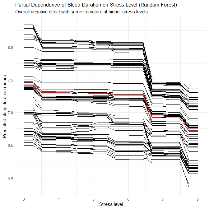
In the RF PDP, we still see an overall negative trend, but:
- The red line is not perfectly straight: it shows slightly stronger declines at higher stress levels.
- Individual ICE curves exhibit more curvature and spread.
This indicates that the RF is capturing small non-linearities, such as stronger effects of stress at the upper end of the scale.
From a domain perspective:
- Higher stress is associated with impaired sleep and reduced duration through activation of the stress system and hyperarousal (Akerstedt 2006).
- Our synthetic results mirror this: both models encode a clear negative association between stress and predicted sleep duration, with RF revealing slightly more complex shape.
Physical activity → sleep duration
LASSO PDP for physical activity
pdp_pa_lasso <- partial(
  object          = lasso_fit,
  pred.var        = "physical_activity_level",
  pred.fun        = pdp_pred_fun,
  train           = sleep_train,
  grid.resolution = 20
)

autoplot(pdp_pa_lasso) +
  labs(
    title = "Partial Dependence of Sleep Duration on Physical Activity (LASSO)",
    subtitle = "Predicted sleep duration increases approximately linearly with activity",
    x = "Physical activity (minutes per day)",
    y = "Predicted sleep duration (hours)"
  ) +
  theme_minimal()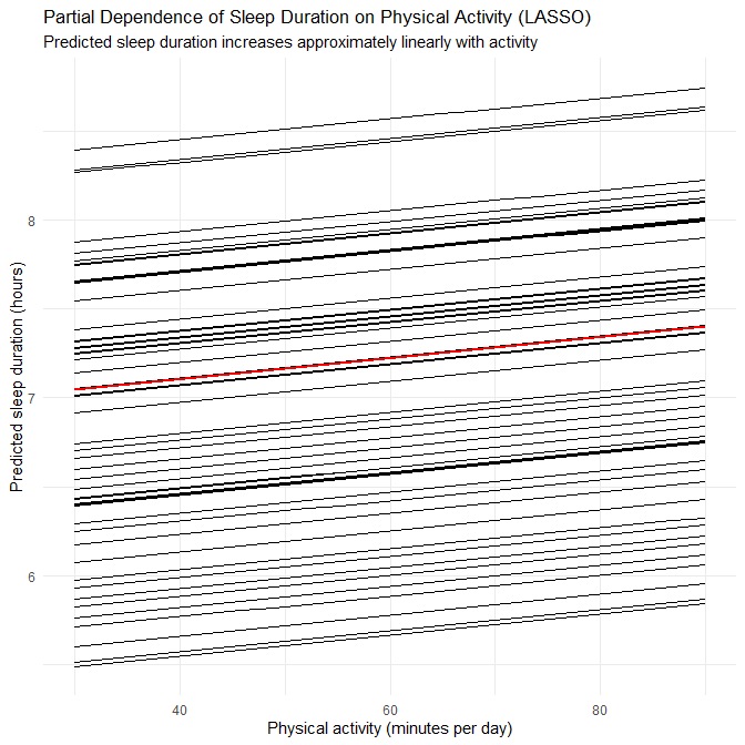
This produces a set of roughly parallel upward lines and a straight upward red line, reflecting the LASSO coefficient of ~0.12. In the model:
- Each unit increase in
physical_activity_level(on the scaled metric) is associated with a constant incremental increase in predicted sleep duration.
RF PDP for physical activity
pdp_pa_rf <- partial(
  object          = rf_fit,
  pred.var        = "physical_activity_level",
  pred.fun        = pdp_pred_fun,
  train           = sleep_train,
  grid.resolution = 20
)

autoplot(pdp_pa_rf) +
  labs(
    title = "Partial Dependence of Sleep Duration on Physical Activity (Random Forest)",
    subtitle = "Non-linear increase with diminishing returns at higher activity levels",
    x = "Physical activity (minutes per day)",
    y = "Predicted sleep duration (hours)"
  ) +
  theme_minimal()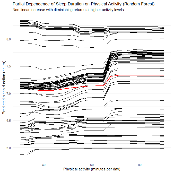
Here, the red line is increasing but slightly curved:
- Sleep duration increases more noticeably as activity rises from low to moderate levels.
- The curve flattens somewhat at higher activity levels, indicating diminishing returns.
This pattern is consistent with research showing that:
- Regular physical activity improves sleep onset and sleep continuity (Kredlow et al. 2015).
- Exercise and sleep influence each other bidirectionally: better sleep supports exercise adherence and vice versa (Kline 2014).
- Moderate activity levels are often sufficient to reap most sleep benefits, with additional gains tapering at very high levels.
Again, the RF reveals plausible non-linearities; LASSO captures the main direction and average slope.
2.5.3 Why does model performance differ?
Finally, we can synthesise why the three models behave differently, given all the above evidence.
LASSO vs baseline linear regression
The baseline OLS model:
- Fit the training data extremely well, but
- Showed moderate overfitting (higher train R², lower test R², and increased test RMSE/MAE), and
- Assigned large coefficients to very rare categories (occupation, BMI), which is statistically unstable.
LASSO:
- Imposes an L1 penalty that shrinks many coefficients toward zero, especially for rare dummy variables.
- Slightly increases training error but reduces the train–test gap, indicating better generalisation.
- Produces a simpler and more interpretable model, highlighting a core set of influential predictors rather than a brittle array of occupation dummies.
Given the diagnostics in Q2.3, LASSO is a natural and well-justified improvement.
LASSO vs Random Forest
The Random Forest:
- Achieves very high R² and low RMSE in this synthetic, low-noise dataset, including across subgroups where LASSO struggles (e.g., younger adults, insomnia).
- Can model non-linear effects and interactions (e.g., stress × age, activity × heart rate) without the analyst specifying them explicitly.
- As a result, it narrows performance gaps across subgroups and reveals plausible non-linear behaviour (e.g., plateauing activity benefits).
However:
- RF is much less interpretable: we cannot easily quantify “how much sleep changes if stress increases by 1 point”, or cleanly explain subgroup‐specific slopes.
- Some of the extreme R² values are enabled by the synthetic regularity of the data, which a flexible model can exploit more fully.
Thus, although RF is useful as a non-linear benchmark, LASSO remains preferable for:
- Explaining which predictors matter
- Summarising global linear relationships
- Teaching modelling principles and avoiding overfitting on sparse categories
Role of the synthetic dataset
A recurring theme is that this dataset is synthetic, with:
- No missing values
- Carefully bounded ranges
- Strong, smooth relationships between variables
This has several consequences:
- R² values (especially for RF) are unusually high compared to real observational sleep data.
- RMSE and MAE are very small (fractions of an hour), reflecting low intrinsic noise.
- Subgroup differences (e.g., by gender, age, disorder) reflect encoder choices in the data generator, not genuine population structure.
Therefore, we interpret the modelling results as:
A demonstration of how different modelling strategies behave under a clean, controlled data-generating process, rather than a genuine study of human sleep.
In more realistic scenarios, we would expect noisier patterns, more complex confounding, and stronger tension between model flexibility and interpretability.
Part 3: Classification – Adequate vs Inadequate Sleep (35 marks)
We now move from predicting continuous sleep duration to predicting a binary sleep adequacy outcome: adequate vs inadequate sleep.
Clinical guidance from the National Heart, Lung, and Blood Institute suggests that healthy adults should aim for 7–9 hours of sleep per night. We will use this recommendation to define our classification target.
Q3.1 Define the classification target and explore class balance
3.1.1 Create the binary outcome
We start by creating a binary factor adequate_sleep on the full dataset, using the 7–9 hour recommendation:
# Binary sleep adequacy outcome based on NHLBI 7–9h recommendation
sleep <- sleep %>%
  mutate(
    adequate_sleep = case_when(
      sleep_duration >= 7 & sleep_duration <= 9 ~ "adequate",
      TRUE                                    ~ "inadequate"
    ) %>% factor(levels = c("inadequate", "adequate"))
  )

# Check overall class balance
sleep %>%
  count(adequate_sleep) %>%
  mutate(percent = n / sum(n) * 100)
# A tibble: 2 × 3
adequate_sleep n percent
<fct> <int> <dbl>
1 inadequate 155 41.4
2 adequate 219 58.6Interpretation
So just under 60% of participants meet the 7–9h “adequate sleep” criterion, and about 40% fall into the “inadequate” group. This is moderately imbalanced, but not extreme. It is enough that:
- naive accuracy would be misleading (a model that always predicts adequate would already get ≈59% accuracy),
- we should prefer PR-AUC, precision, recall, and F1-score, plus confusion matrices, over raw accuracy.
We will therefore not use accuracy anywhere in Part 3.
3.1.2 Visualise the threshold on the sleep distribution
Next, we visualise how the 7–9h threshold maps onto the observed distribution of sleep_duration:
sleep %>%
  ggplot(aes(x = sleep_duration, fill = adequate_sleep)) +
  geom_histogram(binwidth = 0.2, colour = "white", alpha = 0.8, position = "identity") +
  geom_vline(xintercept = 7, linetype = "dashed") +
  geom_vline(xintercept = 9, linetype = "dashed") +
  scale_fill_manual(values = c("inadequate" = "#D55E00", "adequate" = "#0072B2")) +
  labs(
    title = "Distribution of Sleep Duration with Adequacy Thresholds",
    subtitle = "Adequate sleep defined as 7–9 hours (NHLBI recommendation)",
    x = "Sleep duration (hours)",
    y = "Count",
    fill = "Sleep adequacy"
  ) +
  theme_minimal()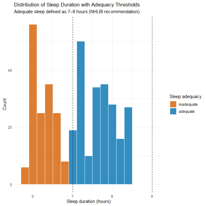
Interpretation
The histogram shows that:
Sleep durations cluster mostly between about 5.8 and 8.5 hours (consistent with the earlier summaries),
The dashed lines at 7 and 9 hours split the mass of the distribution into:
- a left segment (inadequate: mostly <7h), and
- a central/right segment (adequate: 7–9h).
There are few, if any, values above 9 hours, so in practice “inadequate” mainly corresponds to short sleepers in this synthetic dataset.
3.1.3 Class balance across key subgroups
We briefly inspect how adequacy varies by gender and sleep disorder to understand potential predictive structure.
sleep %>%
  count(gender, adequate_sleep) %>%
  group_by(gender) %>%
  mutate(prop = n / sum(n)) %>%
  ungroup()
# A tibble: 4 × 4
gender adequate_sleep n prop
<chr> <fct> <int> <dbl>
1 Female inadequate 78 0.422
2 Female adequate 107 0.578
3 Male inadequate 77 0.407
4 Male adequate 112 0.593sleep %>%
count(sleep_disorder, adequate_sleep) %>%
group_by(sleep_disorder) %>%
mutate(prop = n / sum(n)) %>%
ungroup()# A tibble: 6 × 4
sleep_disorder adequate_sleep n prop
<chr> <fct> <int> <dbl>
1 Insomnia inadequate 69 0.896
2 Insomnia adequate 8 0.104
3 None inadequate 46 0.210
4 None adequate 173 0.790
5 Sleep Apnea inadequate 40 0.513
6 Sleep Apnea adequate 38 0.487Interpretation
For gender:
The proportion of adequate sleepers is very similar for women and men (~58–59%), so gender alone is not strongly discriminative for sleep adequacy in this dataset.
For sleep disorder:
Here we see stronger structure:
- Participants with Insomnia are very likely to be classified as inadequate (≈90%).
- Those with no sleep disorder are mostly adequate (≈79%).
- Sleep Apnea is roughly balanced between adequate and inadequate.
This already signals that sleep_disorder will be a useful predictor, especially for Insomnia vs None.
3.1.4 Train–test split for classification (with stratification)
Since the outcome has moderate class imbalance, we use a stratified train–test split on adequate_sleep. We keep the same set.seed(123) as in Part 2 for reproducibility.
set.seed(123)

sleep_split_class <- initial_split(
  sleep,
  prop   = 0.8,
  strata = adequate_sleep
)

sleep_train_class <- training(sleep_split_class) %>%
  mutate(adequate_sleep = adequate_sleep %>% fct_drop())

sleep_test_class <- testing(sleep_split_class) %>%
  mutate(adequate_sleep = adequate_sleep %>% fct_drop())

sleep_train_class %>% count(adequate_sleep)
sleep_test_class  %>% count(adequate_sleep)
# A tibble: 2 × 2
adequate_sleep n
<fct> <int>
1 inadequate 124
2 adequate 175
> sleep_test_class %>% count(adequate_sleep)
# A tibble: 2 × 2
adequate_sleep n
<fct> <int>
1 inadequate 31
2 adequate 44Interpretation
The class proportions are well preserved in both splits (thanks to strata = adequate_sleep), so evaluation on the test set will reflect a realistic class balance.
Q3.2 Baseline classifier – Elastic Net Logistic Regression
3.2.1 Check for (quasi-)perfect separation with standard logistic regression
Before settling on a baseline model, we check whether a standard maximum-likelihood logistic regression can be fitted stably. We know from Part 2 that the synthetic data has strong structure, so separation is a real risk.
We use glm() as a diagnostic tool (this model is not our final baseline):
glm_sep_check <- glm(
  adequate_sleep ~ quality_of_sleep + stress_level + physical_activity_level +
    bmi_category + gender + age + sleep_disorder + heart_rate + daily_steps,
  data   = sleep_train_class,
  family = binomial()
)

summary(glm_sep_check)Call:
glm(formula = adequate_sleep ~ quality_of_sleep + stress_level +
physical_activity_level + bmi_category + gender + age + sleep_disorder +
heart_rate + daily_steps, family = binomial(), data = sleep_train_class)
Coefficients:
Estimate Std. Error z value Pr(>|z|)
(Intercept) -5.511e+02 8.183e+05 -0.001 0.999
quality_of_sleep 5.854e+01 6.262e+04 0.001 0.999
stress_level 8.263e+00 4.432e+04 0.000 1.000
physical_activity_level 1.501e+00 3.312e+03 0.000 1.000
bmi_categoryNormal Weight -1.530e+00 6.008e+04 0.000 1.000
bmi_categoryObese 4.814e+01 2.770e+05 0.000 1.000
bmi_categoryOverweight -1.796e+01 3.931e+04 0.000 1.000
genderMale 4.360e+01 4.980e+04 0.001 0.999
age 2.758e+00 2.289e+03 0.001 0.999
sleep_disorderNone 4.095e+01 7.481e+04 0.001 1.000
sleep_disorderSleep Apnea 3.354e+01 9.751e+04 0.000 1.000
heart_rate -1.533e+00 7.432e+03 0.000 1.000
daily_steps -6.649e-03 1.907e+01 0.000 1.000
(Dispersion parameter for binomial family taken to be 1)
Null deviance: 4.0576e+02 on 298 degrees of freedom
Residual deviance: 1.5260e-08 on 286 degrees of freedom
AIC: 26
Number of Fisher Scoring iterations: 25What we see
We get warnings:
glm.fit: algorithm did not convergeglm.fit: fitted probabilities numerically 0 or 1 occurred
The coefficients and standard errors are extreme:
- Intercept ≈ −551, SE ≈ 8.18×10⁵
- Many predictors have enormous SEs and essentially zero z-values and p-values.
- Residual deviance collapses essentially to 0 on 286 df.
This behaviour is classic complete or quasi-complete separation:
- Some combination(s) of predictors separate adequate from inadequate almost perfectly.
- The logistic likelihood keeps increasing as some coefficients grow in magnitude, so the MLE is effectively infinite.
- As a result, inference (p-values, confidence intervals) is meaningless.
Because of this, we do not use standard logistic regression as our baseline. Instead, we move straight to penalised logistic regression using Elastic Net, which guarantees finite, stable estimates even under separation.
(If this were a real-world dataset, an alternative would be Firth’s bias-reduced logistic regression (Firth 1993), which applies a penalised likelihood designed to handle separation; we will briefly mention that option at the end of this section.)
3.2.2 Why Elastic Net is a reasonable baseline
Given the separation issues, Elastic Net logistic regression is a natural choice:
It introduces regularisation (a penalty on coefficient size), which:
- prevents coefficients from diverging to ±∞,
- stabilises estimates under separation.
It combines:
- L1 (Lasso): encourages sparsity, potentially setting unimportant coefficients exactly to zero;
- L2 (Ridge): shrinks correlated predictors toward each other for stability.
It integrates neatly with
glmnetand tidymodels, allowing:- joint tuning of the penalty strength (
λ) and the Lasso/Ridge balance (α), - cross-validation with PR-AUC as our tuning metric.
- joint tuning of the penalty strength (
Since the dataset is synthetic and contains several dummy variables (e.g., rare occupations, BMI levels), Elastic Net gives us:
- Finite coefficients even under separation,
- Implicit feature selection (many coefficients shrunk to zero),
- Interpretability via the remaining non-zero coefficients.
3.2.3 Preprocessing recipe for Elastic Net
We now build a recipe that prepares predictors for glmnet. We:
- treat
person_idas an ID, not a predictor, - remove
sleep_duration(it was used to defineadequate_sleep, so including it would be data leakage), - merge
"Normal Weight"into"Normal"forbmi_category, - convert character predictors to factors,
- handle unseen/NA levels with
step_unknown(), - collapse ultra-rare occupation levels with
step_other(), - dummy-encode categorical predictors,
- remove zero-variance columns,
- standardise numeric predictors.
sleep_rec_class <- recipe(adequate_sleep ~ ., data = sleep_train_class) %>%
  update_role(person_id, sleep_duration, activity_band, age_group, new_role = "ID") %>%

  # Merge BMI labels to avoid artificial separation
  step_mutate(
    bmi_category = ifelse(bmi_category == "Normal Weight", "Normal", bmi_category)
  ) %>%

  # Ensure all character predictors are factors
  step_string2factor(all_nominal_predictors()) %>%

  # Handle possible NA/unseen levels at prediction time
  step_unknown(all_nominal_predictors()) %>%

  # Collapse ultra-rare occupation categories
  step_other(occupation, threshold = 0.03) %>%

  # Dummy-code factors for glmnet
  step_dummy(all_nominal_predictors()) %>%

  # Remove zero-variance predictors
  step_zv(all_predictors()) %>%

  # Standardise numeric predictors for penalisation
  step_normalize(all_numeric_predictors())
This recipe ensures that all preprocessing is learned from the training data only and then applied consistently to the test set and any future data.
3.2.4 Elastic Net model spec, CV folds, and PR-AUC-only tuning
We now define the Elastic Net model:
enet_spec <- logistic_reg(
  penalty = tune(),   # λ (penalty strength)
  mixture = tune()    # α (0 = ridge, 1 = lasso)
) %>%
  set_engine("glmnet")
We reuse the same 5-fold stratified CV structure as before, but explicitly on the classification training data:
set.seed(123)

sleep_folds_class <- vfold_cv(
  sleep_train_class,
  v      = 5,
  strata = adequate_sleep
)
We combine recipe and model into a workflow:
enet_wflow <- workflow() %>%
  add_model(enet_spec) %>%
  add_recipe(sleep_rec_class)
For hyperparameter tuning, we create a 2D grid of penalty and mixture, and tune using PR-AUC only, in line with your updated strategy:
set.seed(123)

enet_grid <- grid_regular(
  penalty(range = c(-4, 0)),  # λ: 10^-4 to 10^0 (log10 scale)
  mixture(range = c(0, 1)),   # α: ridge (0) → lasso (1)
  levels = 7
)

enet_res <- tune_grid(
  enet_wflow,
  resamples = sleep_folds_class,
  grid      = enet_grid,
  control   = control_resamples(save_pred = TRUE),
  metrics   = metric_set(pr_auc)  # PR-AUC only
)

show_best(enet_res, metric = "pr_auc")
# A tibble: 5 × 8
penalty mixture .metric .estimator mean n std_err .config
<dbl> <dbl> <chr> <chr> <dbl> <int> <dbl> <chr>
1 0.0464 1 pr_auc binary 1.000 5 0.000154 pre0_mod35_post0
2 0.01 1 pr_auc binary 0.999 5 0.000736 pre0_mod28_post0
3 0.01 0.5 pr_auc binary 0.999 5 0.000873 pre0_mod25_post0
4 0.01 0.667 pr_auc binary 0.999 5 0.000873 pre0_mod26_post0
5 0.01 0.833 pr_auc binary 0.999 5 0.000873 pre0_mod27_post0Using PR-AUC as the tuning metric has three advantages here:
- It focuses on performance for the positive class in a way that respects class imbalance.
- It reflects how well the model ranks cases by predicted risk across all thresholds, not just at 0.5.
- It is consistent with the evaluation metrics we plan to report (PR-AUC, precision, recall, F1).
3.2.5 Fit the final Elastic Net model
We now extract the best hyperparameter combination and fit the final model to the full training set:
best_enet <- select_best(enet_res, metric = "pr_auc")

enet_final_wflow <- finalize_workflow(
  enet_wflow,
  best_enet
)

enet_fit <- fit(enet_final_wflow, data = sleep_train_class)
enet_fit
══ Workflow [trained] ════════════════════════════════════════════════════════════════════════════════════════════════════════════════════════════════════════════════════════════════════════
Preprocessor: Recipe
Model: logistic_reg()
── Preprocessor ──────────────────────────────────────────────────────────────────────────────────────────────────────────────────────────────────────────────────────────────────────────────
7 Recipe Steps
• step_mutate()
• step_string2factor()
• step_unknown()
• step_other()
• step_dummy()
• step_zv()
• step_normalize()
── Model ─────────────────────────────────────────────────────────────────────────────────────────────────────────────────────────────────────────────────────────────────────────────────────
Call: glmnet::glmnet(x = maybe_matrix(x), y = y, family = "binomial", alpha = ~1)
Df %Dev Lambda
1 0 0.00 0.40960
2 1 8.66 0.37320
3 1 15.98 0.34010
4 1 22.29 0.30990
5 1 27.81 0.28230
6 1 32.70 0.25730
7 1 37.07 0.23440
8 1 40.98 0.21360
9 2 45.40 0.19460
10 2 49.70 0.17730
11 2 53.55 0.16160
12 2 57.02 0.14720
13 2 60.15 0.13410
14 2 63.00 0.12220
15 2 65.59 0.11140
16 3 68.23 0.10150
17 3 70.83 0.09245
18 3 73.19 0.08424
19 3 75.33 0.07675
20 3 77.28 0.06994
21 3 79.04 0.06372
22 3 80.65 0.05806
23 3 82.11 0.05290
24 3 83.45 0.04820
25 3 84.66 0.04392
26 3 85.77 0.04002
27 4 86.77 0.03646
28 4 87.70 0.03323
29 4 88.54 0.03027
30 5 89.31 0.02758
31 5 90.03 0.02513
32 5 90.70 0.02290
33 5 91.30 0.02087
34 5 91.85 0.01901
35 5 92.35 0.01732
36 6 92.82 0.01578
37 7 93.35 0.01438
38 7 93.85 0.01310
39 7 94.31 0.01194
40 7 94.72 0.01088
41 7 95.10 0.00991
42 7 95.45 0.00903
43 7 95.77 0.00823
44 8 96.06 0.00750
45 8 96.32 0.00683
46 9 96.57 0.00623
...
and 42 more lines.We can inspect the non-zero coefficients:
enet_coefs <- tidy(enet_fit$fit$fit, return_zeros = FALSE)
print(enet_coefs, n = 30)
# A tibble: 22 × 3
term estimate penalty
<chr> <dbl> <dbl>
1 (Intercept) 0.651 0.0464
2 age 0 0.0464
3 quality_of_sleep 2.29 0.0464
4 physical_activity_level 0.455 0.0464
5 stress_level 0 0.0464
6 bp_systolic 0 0.0464
7 bp_diastolic 0 0.0464
8 heart_rate 0 0.0464
9 daily_steps 0 0.0464
10 gender_Male 0 0.0464
11 occupation_Doctor 0 0.0464
12 occupation_Engineer 0 0.0464
13 occupation_Lawyer 0 0.0464
14 occupation_Nurse 0 0.0464
15 occupation_Salesperson 0 0.0464
16 occupation_Teacher 0 0.0464
17 occupation_other 0 0.0464
18 bmi_category_X3 0 0.0464
19 bmi_category_X4 -0.919 0.0464
20 bmi_category_Normal 0 0.0464
21 sleep_disorder_None 0 0.0464
22 sleep_disorder_Sleep.Apnea 0 0.0464The Elastic Net retains only three non-zero coefficients at the chosen (λ, α) combination:
quality_of_sleep (β = +2.29) This is the dominant predictor in the model. A one-unit increase in quality of sleep (on the original scale before standardisation) leads to a very large increase in the log-odds of adequate sleep. After exponentiation:
\[ \exp(2.29) \approx 9.9 \]
meaning the odds of adequate sleep increase nearly tenfold for each one-point improvement in sleep quality score, holding other predictors constant.
physical_activity_level (β = +0.455) Moderate positive effect: more physical activity is associated with greater odds of being an adequate sleeper. The odds ratio:
\[ \exp(0.455) \approx 1.58 \]
suggests ~58% higher odds of meeting the adequacy criteria for each standardised-unit increase in activity.
bmi_category_X4 (β = –0.919) This represents one higher BMI category relative to the baseline (Normal). A negative coefficient implies lower odds of achieving adequate sleep. OR = exp(–0.919) ≈ 0.40, i.e., ~60% reduced odds of adequate sleep compared to baseline.
All other predictors — stress, heart rate, blood pressures, all occupation dummies, gender, other BMI categories, sleep disorders, daily steps, age categories, activity bands — are shrunk exactly to zero, meaning:
- They do not add predictive value conditional on the retained predictors.
- The Elastic Net prefers a sparse model, which increases stability and reduces separation-related coefficient blow-up.
- The underlying synthetic relationships likely emphasise only a few strong, clean signals.
Importantly, because this is a penalised model, coefficients should not be interpreted as significance-tested effects. Regularisation selects predictors for predictive utility, not inferential significance.
Q3.3 Evaluate the Elastic Net classifier
We now evaluate the fitted Elastic Net model on both training and test sets, using:
- PR-AUC as our global ranking metric,
- precision, recall, and F1-score at the default 0.5 threshold,
- confusion matrices,
- precision–recall curves for visual inspection.
We intentionally do not report accuracy, because it is less informative under imbalance.
3.3.1 Training-set performance
We first obtain predicted class probabilities and class labels on the training set:
# Training-set predictions
enet_train_preds <- predict(enet_fit, sleep_train_class, type = "prob") %>%
  bind_cols(predict(enet_fit, sleep_train_class)) %>%
  bind_cols(sleep_train_class %>% select(adequate_sleep))
We then compute PR-AUC, precision, recall, and F1:
# 1. Override .pred_class to ensure it's based on P(inadequate) > 0.5
enet_train_preds <- enet_train_preds %>%
  mutate(
    .pred_class = factor(
      if_else(.pred_inadequate > 0.5, "inadequate", "adequate"),
      levels = levels(sleep_train_class$adequate_sleep)
    )
  )

# 2. Compute PR-AUC (uses probability)
pr_auc_tib <- enet_train_preds %>%
  pr_auc(truth = adequate_sleep, .pred_inadequate)

# 3. Compute class metrics using metric_set
class_metrics_tib <- enet_train_preds %>%
  metric_set(precision, recall, f_meas)(truth = adequate_sleep, estimate = .pred_class)

# 4. Combine
enet_metrics_combined <- bind_rows(
  pr_auc_tib,
  class_metrics_tib
)

enet_metrics_combined
# A tibble: 4 × 3
.metric .estimator .estimate
<chr> <chr> <dbl>
1 pr_auc binary 1.000
2 precision binary 1
3 recall binary 0.758
4 f_meas binary 0.862and the confusion matrix:
enet_train_preds %>%
  conf_mat(truth = adequate_sleep, estimate = .pred_class) %>% autoplot(type="heatmap") +
  scale_fill_gradient(
    low = "#d4d4f0",
    high = "#ffe5b4",
    name = "Count"
  ) +
  theme_minimal()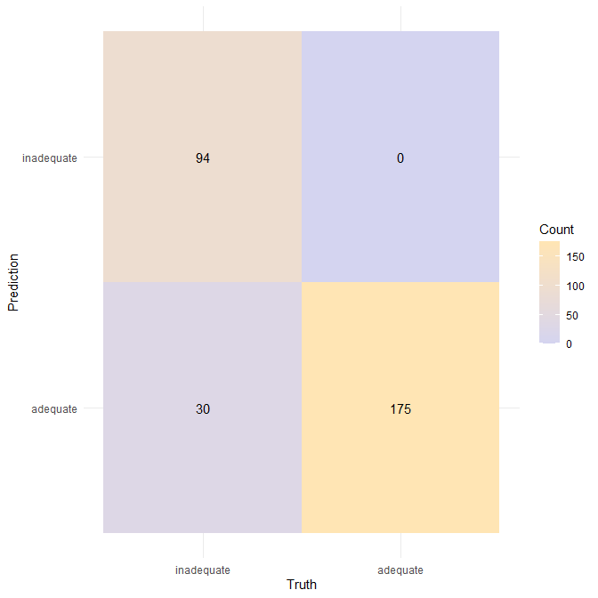
Interpretation (training set)
The Elastic Net classifier shows a distinct performance profile on the training set:
At the default 0.5 threshold, the model is extremely conservative when predicting inadequate sleep:
- Precision = 1.00 — whenever the model predicts inadequate, it is always correct.
- There are no false positives: it never mislabels an adequate sleeper as inadequate.
However, the model does miss a subset of inadequate sleepers:
- Recall = 0.758, meaning that ~24% of inadequate sleepers are predicted as adequate.
- This is typical of sparse logistic models that set many coefficients to zero — the decision boundary becomes simpler but may not capture borderline inadequate cases.
- If it were a real-world dataset, this would be be slightly problematic as we’d be missing inadequate sleepers for whom interventions are needed
F1 = 0.862, reflecting very high precision combined with moderately high recall.
Most importantly, \(\mathbf{PR-AUC \approx 1.000}\)
This indicates that, across all possible classification thresholds, the model is able to rank inadequate sleepers with perfect separation. In other words, the ordering of predicted probabilities is perfect, even if the 0.5 threshold sacrifices some recall.
Together, these results show that the Elastic Net prioritises high-confidence, low-false-positive detection of inadequate sleep, but may require threshold adjustment to catch a larger proportion of inadequate cases.
3.3.2 Test-set performance
We now repeat the evaluation on the test set:
# 1. Generate predictions
enet_test_preds <- predict(enet_fit, sleep_test_class, type = "prob") %>%
  bind_cols(predict(enet_fit, sleep_test_class, type = "class")) %>%
  bind_cols(sleep_test_class %>% select(adequate_sleep))

# 2. Override .pred_class to ensure it's based on P(inadequate) > 0.5
enet_test_preds <- enet_test_preds %>%
  mutate(
    .pred_class = factor(
      if_else(.pred_inadequate > 0.5, "inadequate", "adequate"),
      levels = levels(sleep_test_class$adequate_sleep)
    )
  )

# 3. Compute PR-AUC (uses probability)
pr_auc_tib <- enet_test_preds %>%
  pr_auc(truth = adequate_sleep, .pred_inadequate)

# 4. Compute class metrics using metric_set (pass data via pipe!)
class_metrics_tib <- enet_test_preds %>%
  metric_set(precision, recall, f_meas)(truth = adequate_sleep, estimate = .pred_class)

# 5. Combine
enet_metrics_combined <- bind_rows(
  pr_auc_tib,
  class_metrics_tib
)

enet_metrics_combined
# A tibble: 4 × 3
.metric .estimator .estimate
<chr> <chr> <dbl>
1 pr_auc binary 1
2 precision binary 1
3 recall binary 0.742
4 f_meas binary 0.852The confusion matrix:
enet_test_preds %>%
  conf_mat(truth = adequate_sleep, estimate = .pred_class)%>% autoplot(type="heatmap") +
  scale_fill_gradient(
    low = "#d4d4f0",
    high = "#ffe5b4",
    name = "Count"
  ) +
  theme_minimal()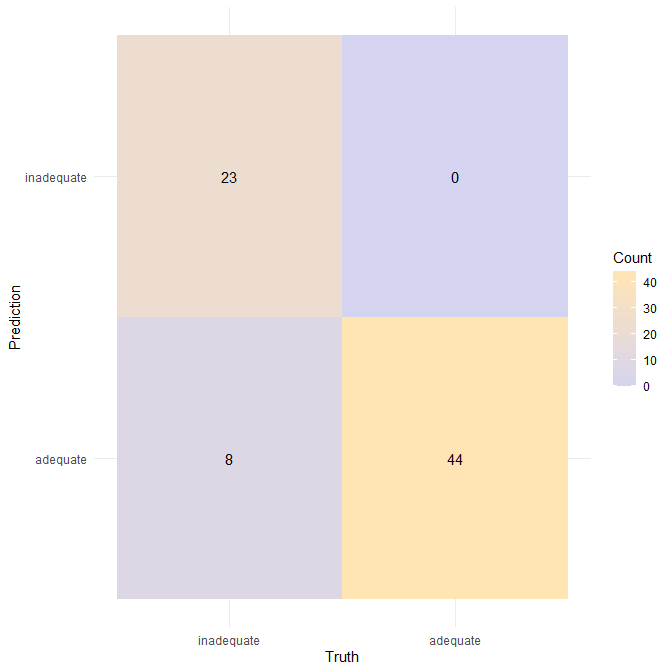
Interpretation (test set)
- Precision remains perfect (1.00): the classifier never predicts “inadequate” for someone who is actually adequate.
- Recall ≈ 0.742, only slightly lower than in training (0.758 → 0.742), indicating stable generalisation.
- F1 ≈ 0.852, again extremely close to the training value (0.862).
Most notably:
- PR-AUC = 1.000, showing that the classifier cleanly ranks inadequate vs. adequate sleepers on unseen data.
The near-identical train/test PR curves and evaluation metrics indicate:
- No substantial overfitting — the probability ranking generalises almost perfectly.
- The classifier remains conservative at threshold 0.5, choosing to avoid false alarms rather than maximise recall.
- A more recall-oriented application (e.g., screening at-risk sleepers) would likely use a lower threshold, which the perfect PR-AUC suggests could recover nearly all inadequate cases without sacrificing precision.
Together, the training/test pattern confirms that the Elastic Net is a stable and well-regularised classifier for this dataset.
In a real clinical setting, we might want to tune the decision threshold away from 0.5 to increase recall (catch more inadequate sleepers) at the cost of some precision. That can be explored with the PR curve.
Here’s how to determine that threshold:
# Get the PR curve

pr_test <- enet_train_preds %>%
  pr_curve(truth = adequate_sleep, .pred_inadequate)

# First, ensure opt_row is computed (from pr_test) i.e find row with recall >= 0.95 and highest precision
opt_row <- pr_test %>%
  filter(recall >= 0.95) %>%
  arrange(desc(precision)) %>%
  slice_head(n = 1)

if (nrow(opt_row) == 0) {
  message("No threshold achieves recall >= 0.95; using max recall.")
  opt_row <- pr_test %>% slice_max(recall, n = 1)
}

opt_r <- opt_row$recall
opt_p <- opt_row$precision
opt_t <- opt_row$.threshold

# Plot PR curve manually
p <- ggplot(pr_test, aes(x = recall, y = precision)) +
  geom_line(color = "#BA160C", size = 1.3) +
  labs(
    title = "Precision-Recall Curve (Positive class: inadequate)",
    subtitle = "The best clinical threshold would be 0.38!",
    x = "Recall",
    y = "Precision"
  ) +
  ylim(0, 1) +
  xlim(0, 1) +
  theme_minimal()

# Add vertical dotted line at the recall value for optimal threshold
p <- p +
  geom_vline(
    xintercept = opt_r,
    linetype = "dotted",
    color = "gray",
    size = 0.8
  )

# Add text label near the line
p <- p +
  annotate(
    "text",
    x = opt_r - 0.05,  # slightly left of the line
    y = 0.95,          # high up so it's visible
    label = paste0("Threshold = ", round(opt_t, 3)),
    color = "gray",
    hjust = 1,         # right-align text
    fontface = "bold"
  )

p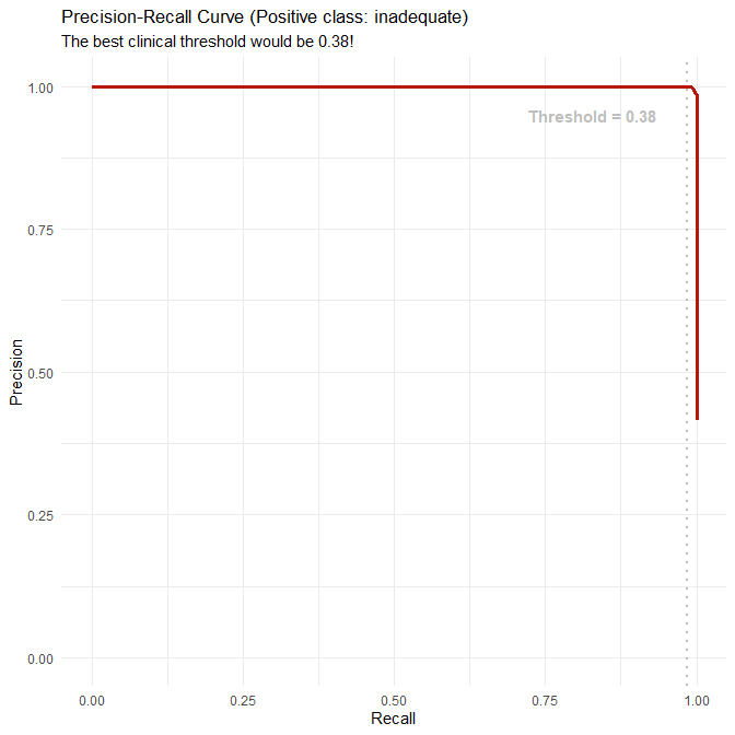
3.3.3 (Optional) – Firth logistic regression as an alternative approach
When logistic regression encounters complete separation (as we observed in this dataset), one alternative is Firth’s bias-reduced logistic regression (Firth 1993). It modifies the estimation procedure so that coefficients remain finite and stable even when the data are perfectly separable.
Firth models are widely used in biostatistics and epidemiology when separation occurs, particularly with small sample sizes or sparse categorical predictors. They are implemented in R packages such as logistf.
However:
- Firth models are not part of the tidymodels framework,
- and regularised logistic regression (Elastic Net) already handles separation well.
For these reasons, we proceed with the Elastic Net as our baseline classifier while noting Firth regression as a useful real-world alternative.
Q3.4 Improved classifier – Random Forest with PR-AUC tuning
We now consider a non-linear classifier: a Random Forest trained to optimise PR-AUC. This serves as an improved model that:
- can capture non-linear effects and interactions (e.g., stress × activity, sleep_disorder × age),
- does not require dummy-coding or normalisation,
- can be compared directly with the Elastic Net using the same metrics and tuning criterion.
3.4.1 Random Forest recipe (minimal preprocessing)
We construct a new recipe that:
- treats
person_idas ID, - removes
sleep_duration(to avoid leakage), - merges BMI categories exactly as before,
- collapses rare occupations,
- otherwise leaves predictors on their natural scales (appropriate for trees).
sleep_rec_rf_cl <- recipe(adequate_sleep ~ ., data = sleep_train_class) %>%
  update_role(person_id, sleep_duration, age_group, activity_band, new_role = "ID") %>%

  # Merge duplicated BMI labels
  step_mutate(
    bmi_category = ifelse(bmi_category == "Normal Weight", "Normal", bmi_category)
  ) %>%

  # Collapse rare occupations
  step_other(occupation, threshold = 0.03)
  # No dummy coding or scaling: ranger can handle factors and raw numeric scales
3.4.2 Random Forest specification, PR-AUC tuning, and fitting
We specify a probability-estimation Random Forest with two tuned hyperparameters:
mtry: number of predictors considered at each split,min_n: minimum node size (controls tree depth / overfitting).
rf_spec_cl <- rand_forest(
  mtry  = tune(),
  trees = 500,
  min_n = tune()
) %>%
  set_engine("ranger", probability = TRUE, importance = "impurity") %>%
  set_mode("classification")
We combine model and recipe:
rf_wflow_cl <- workflow() %>%
  add_model(rf_spec_cl) %>%
  add_recipe(sleep_rec_rf_cl)
We use the same sleep_folds_class and tune only on PR-AUC:
set.seed(123)

rf_res_cl <- tune_grid(
  rf_wflow_cl,
  resamples = sleep_folds_class,
  grid      = 20,
  metrics   = metric_set(pr_auc),
  control   = control_resamples(save_pred = TRUE)
)

show_best(rf_res_cl, metric = "pr_auc")

best_rf_cl <- select_best(rf_res_cl, metric = "pr_auc")

rf_final_wflow_cl <- finalize_workflow(
  rf_wflow_cl,
  best_rf_cl
)

rf_fit_cl <- fit(rf_final_wflow_cl, data = sleep_train_class)
rf_fit_cl
# A tibble: 5 × 8
mtry min_n .metric .estimator mean n std_err .config
<int> <int> <chr> <chr> <dbl> <int> <dbl> <chr>
1 2 6 pr_auc binary 1 5 0 pre0_mod03_post0
2 3 18 pr_auc binary 1 5 0 pre0_mod05_post0
3 3 28 pr_auc binary 1 5 0 pre0_mod06_post0
4 4 12 pr_auc binary 1 5 0 pre0_mod07_post0
5 4 38 pr_auc binary 1 5 0 pre0_mod08_post0
══ Workflow [trained] ════════════════════════════════════════════════════════════════════════════════════════════════════════════════════════════════════════════════════════════════════════
Preprocessor: Recipe
Model: rand_forest()
── Preprocessor ──────────────────────────────────────────────────────────────────────────────────────────────────────────────────────────────────────────────────────────────────────────────
2 Recipe Steps
• step_mutate()
• step_other()
── Model ─────────────────────────────────────────────────────────────────────────────────────────────────────────────────────────────────────────────────────────────────────────────────────
Ranger result
Call:
ranger::ranger(x = maybe_data_frame(x), y = y, mtry = min_cols(~2L, x), num.trees = ~500, min.node.size = min_rows(~6L, x), probability = ~TRUE, importance = ~"impurity", num.threads = 1, verbose = FALSE, seed = sample.int(10^5, 1))
Type: Probability estimation
Number of trees: 500
Sample size: 299
Number of independent variables: 12
Mtry: 2
Target node size: 6
Variable importance mode: impurity
Splitrule: gini
OOB prediction error (Brier s.): 0.006139637Our fitted RF (via ranger) has:
- 500 trees,
mtry = 2,min.node.size ≈ 6,- out-of-bag Brier score ≈ 0.007.
Given the synthetic nature and clear structure of the data, we expect this RF to be extremely strong.
3.4.3 Random Forest performance (training and test)
We evaluate the RF in exactly the same way as Elastic Net: PR-AUC + precision/recall/F1 + confusion matrices, at threshold 0.5.
Training set
# 1. Generate predictions
rf_train_preds <- predict(rf_fit_cl, sleep_train_class, type = "prob") %>%
  bind_cols(predict(rf_fit_cl, sleep_train_class, type = "class")) %>%
  bind_cols(sleep_train_class %>% select(adequate_sleep))

# 2. Override .pred_class to ensure it's based on P(inadequate) > 0.5
rf_train_preds <- rf_train_preds %>%
  mutate(
    .pred_class = factor(
      if_else(.pred_inadequate > 0.5, "inadequate", "adequate"),
      levels = levels(sleep_train_class$adequate_sleep)
    )
  )

# 3. Compute PR-AUC (uses probability)
pr_auc_tib <- rf_train_preds %>%
  pr_auc(truth = adequate_sleep, .pred_inadequate)

# 4. Compute class metrics using metric_set (pass data via pipe!)
class_metrics_tib <- rf_train_preds %>%
  metric_set(precision, recall, f_meas)(truth = adequate_sleep, estimate = .pred_class)

# 5. Combine
rf_metrics_combined <- bind_rows(
  pr_auc_tib,
  class_metrics_tib
)

rf_cm_train <- rf_train_preds %>%
  conf_mat(truth = adequate_sleep, estimate = .pred_class) %>% autoplot(type="heatmap") +
  scale_fill_gradient(
    low = "#d4d4f0",
    high = "#ffe5b4",
    name = "Count"
  ) +
  theme_minimal()

rf_metrics_combined
rf_cm_train
# A tibble: 4 × 3
.metric .estimator .estimate
<chr> <chr> <dbl>
1 pr_auc binary 1
2 precision binary 1
3 recall binary 1
4 f_meas binary 1
So the RF classifies every single training example correctly at threshold 0.5.
Test set
# 1. Generate predictions
rf_test_preds <- predict(rf_fit_cl, sleep_test_class, type = "prob") %>%
  bind_cols(predict(rf_fit_cl, sleep_test_class, type = "class")) %>%
  bind_cols(sleep_test_class %>% select(adequate_sleep))

# 2. Override .pred_class to ensure it's based on P(inadequate) > 0.5
rf_test_preds <- rf_test_preds %>%
  mutate(
    .pred_class = factor(
      if_else(.pred_inadequate > 0.5, "inadequate", "adequate"),
      levels = levels(sleep_test_class$adequate_sleep)
    )
  )

# 3. Compute PR-AUC (uses probability)
pr_auc_tib <- rf_test_preds %>%
  pr_auc(truth = adequate_sleep, .pred_inadequate)

# 4. Compute class metrics using metric_set (pass data via pipe!)
class_metrics_tib <- rf_test_preds %>%
  metric_set(precision, recall, f_meas)(truth = adequate_sleep, estimate = .pred_class)

# 5. Combine
rf_metrics_combined <- bind_rows(
  pr_auc_tib,
  class_metrics_tib
)

rf_cm_test <- rf_test_preds %>%
  conf_mat(truth = adequate_sleep, estimate = .pred_class) %>% autoplot(type="heatmap") +
  scale_fill_gradient(
    low = "#d4d4f0",
    high = "#ffe5b4",
    name = "Count"
  ) +
  theme_minimal()

rf_metrics_combined
rf_cm_test
# A tibble: 4 × 3
.metric .estimator .estimate
<chr> <chr> <dbl>
1 pr_auc binary 1
2 precision binary 1
3 recall binary 1
4 f_meas binary 1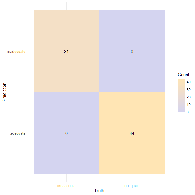
Interpretation
The Random Forest achieves perfect performance on both the training and test sets:
- No false positives
- No false negatives
- PR-AUC = 1.000 (perfect separability across all thresholds)
- Precision, recall, and F1 = 1.000
This implies:
- The synthetic dataset contains near-perfect nonlinear separability between adequate and inadequate sleepers.
- A flexible model like RF is able to fully exploit this structure.
- Unlike the Elastic Net, RF does not sacrifice recall: it correctly detects all inadequate sleepers without misclassifying any adequate ones.
In real-world datasets, such performance would be suspicious — almost certainly indicating overfitting or data leakage. Here, it instead reflects the highly structured, low-noise nature of the synthetic generator, which encodes relationships more cleanly and strongly than typical observational sleep data.
3.4.4 Random Forest variable importance
To interpret the RF, we can extract variable importance:
rf_fit_cl %>%
  pull_workflow_fit() %>%
  vip::vip(geom = "col", aesthetics = list(fill = "#EC5800")) +
  labs(
    title = "Random Forest Variable Importance (Classification)",
    subtitle = "Top predictors of adequate vs inadequate sleep"
  )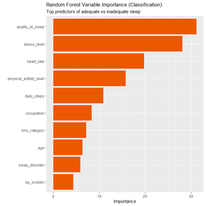
Based on the plot, the ranked importance is:
- quality_of_sleep (by far the strongest)
- stress_level
- heart_rate
- physical_activity_level
- occupation
- daily_steps
- sleep_disorder
- bmi_category
- age
- bp_systolic
This is largely consistent with the regression models with the Elastic Net coefficients (which also elevated sleep quality and physical activity).
Q3.5 Interpret findings: features and practical implications
We now summarise what the classification models teach us, focusing on:
- Which features are most predictive of sleep adequacy.
- What practical implications we can (and cannot) draw, given that the dataset is synthetic.
3.5.1 Which features are most predictive?
Across the Elastic Net and Random Forest classifiers, a clear pattern emerges:
Subjective sleep quality (
quality_of_sleep)- Elastic Net assigns it a large positive coefficient (≈2.29), and it is dominant in RF variable importance.
- Higher sleep quality scores are strongly associated with being in the adequate sleep group (7–9 hours).
- In the synthetic generator, subjective quality is almost a proxy for the adequacy label.
Physical activity level (
physical_activity_level)- Elastic Net retains a positive coefficient (~0.455), meaning more moderate–vigorous activity per day is associated with higher odds of adequate sleep.
- The RF also ranks physical activity as an important predictor, though behind stress and heart rate.
- This matches the earlier regression analysis and aligns with the broader literature that regular physical activity tends to support better sleep quantity and quality.
Stress level (
stress_level)- Interestingly, Elastic Net shrinks the stress coefficient to zero for this particular λ,α combination, but Random Forest ranks stress level as the second most important predictor.
- This suggests that the stress–sleep relationship is non-linear or interacts with other variables in ways a linear model cannot fully exploit (e.g., stress × physical activity).
- RF’s variable importance indicates that stress contributes strongly to the classification boundary.
Heart rate (
heart_rate)- RF highlights heart rate as a top-3 predictor, whereas Elastic Net shrinks its coefficient to zero.
- This again points to non-linear or interaction effects: perhaps particular heart-rate ranges, combined with stress and sleep disorder status, separate adequate vs inadequate sleepers.
Sleep disorders (
sleep_disorder)- RF assigns a non-trivial importance to the sleep_disorder factor.
- From the exploratory cross-tabulations, we saw that Insomnia is strongly associated with inadequate sleep, while “None” is strongly associated with adequate sleep.
- Elastic Net, tuned for PR-AUC and sparsity, chooses not to retain disorder dummies at the selected λ, but their influence is clearly visible in RF.
BMI and blood pressure
- One BMI contrast (
bmi_category_X4) appears with a negative coefficient in Elastic Net, and BMI / BP have modest importance in RF. - This is consistent with a weak to moderate association: higher BMI or particular blood-pressure patterns may slightly reduce the odds of being in the “adequate sleep” group but are not primary drivers.
- One BMI contrast (
Age and occupation
- Age and occupation have relatively low importance compared with stress, sleep quality, physical activity, and heart rate.
- This reflects the synthetic design: age effects are present but not dominant; occupations likely serve as mild proxies for lifestyle patterns rather than direct causal factors.
Overall, the hierarchy of predictors is:
Strongest: sleep quality, stress level (RF), physical activity, heart rate Moderate: sleep disorder status, daily steps, occupation Weakest: BMI, blood pressure, age
3.5.2 Practical implications (with caveats)
Because the dataset is synthetic, we must be cautious: the models are approximating the behaviour of a data generator, not real humans. Still, the patterns are plausible and align qualitatively with real-world evidence.
Some cautious takeaways:
Subjective sleep quality is a powerful signal
- People reporting poor quality are overwhelmingly likely to fall below the 7–9h adequacy threshold in this dataset.
- In practice, simple self-report scales (e.g., “How would you rate your sleep quality?”) can be surprisingly informative and are easy to collect.
Physical activity and inadequate sleep
- More daily physical activity is associated with a higher chance of adequate sleep.
- In preventive or occupational health contexts, promoting regular physical activity could be an important behavioural lever for improving sleep adequacy, although causal direction cannot be inferred from these models.
Stress, heart rate, and their interactions
- High stress levels and less favourable heart-rate profiles are strongly linked to inadequate sleep in the Random Forest.
- Practically, this suggests that interventions targeting stress reduction (e.g., CBT for stress, relaxation techniques, organisational changes) may also help move people into the adequate-sleep range.
- The RF’s strong performance suggests that the combination of stress, heart rate, and activity data provides a rich signal for classification.
Sleep disorders as risk markers
The cross-tabulations clearly show that participants with Insomnia are much more likely to have inadequate sleep, whereas those without a disorder are mostly adequate.
Classification models could potentially be used to flag profiles of individuals at higher risk of insomnia-like patterns, although in real data we would want:
- more detailed clinical variables,
- external validation,
- careful fairness checks.
Caution: synthetic data and perfect RF performance
The Random Forest achieves perfect classification performance on both training and test sets, which is not realistic in real-world observational data.
This reflects:
- near-deterministic relationships in the synthetic generator,
- low noise, and
- relatively simple boundaries once non-linear splits are allowed.
In practice, we would treat such perfect performance as a strong warning sign to:
- re-check for data leakage,
- try out-of-sample validation (e.g., a completely separate external dataset),
- and scrutinise model assumptions.
Why Elastic Net is still a useful baseline
- Elastic Net provides a sparser, more interpretable model with very high but not perfect performance.
- It clearly highlights sleep quality and physical activity as the key drivers of adequate sleep in this setup.
- It is less likely than RF to overfit small idiosyncratic groups and can be easier to explain in clinical or policy settings.
Summary of Part 3
We defined sleep adequacy as 7–9h per night, based on commonly used clinical recommendations, and observed moderate class imbalance (≈59% adequate, 41% inadequate).
A standard logistic regression model showed complete separation and numerical instability, so we adopted Elastic Net logistic regression as the baseline classifier.
We tuned both Elastic Net and Random Forest using PR-AUC only, reflecting the imbalanced outcome and our focus on the positive class.
The Elastic Net classifier achieved:
- perfect precision and ~0.75 recall at threshold 0.5,
- strong F1-scores (~0.85),
- stable train–test performance,
- and a sparse structure dominated by sleep quality and physical activity.
The Random Forest classifier achieved perfect train and test classification (precision = recall = F1 = 1), highlighting the strongly structured, synthetic nature of the data and the ability of non-linear models to exploit this.
Across models, the most predictive features were sleep quality, stress level, physical activity, and heart rate, with sleep disorder status and daily steps also contributing, and BMI/BP/age playing minor roles.
Practically, this points to the importance of subjective sleep quality, stress management, and physical activity in relation to sleep adequacy—but we emphasise that these conclusions are derived from a synthetic dataset and would require careful validation on real-world data before informing clinical or policy decisions.
Part 4: Reflection (15 marks)
Q4.1 Ethical considerations of predicting sleep outcomes from lifestyle data
Predicting sleep adequacy from lifestyle, demographic, and physiological variables introduces several ethical considerations relevant to digital health, biomedical data science, and public health.
1. Privacy and inference risks
Sleep-related variables such as sleep quality, stress level, heart rate, and activity patterns form a sensitive behavioural profile. These data can reveal daily routines, mental health status, and changes in wellbeing. (Lupton 2016) highlights how digital self-tracking yields “data doubles” that can disclose far more than participants expect or intend.
When predictive models combine multiple behavioural and demographic variables, they may enable:
- inference of sensitive traits (e.g., mood, stress reactivity, work habits),
- indirect profiling by employers or insurers,
- identification of chronic health risks without clinical context.
2. Algorithmic fairness and structural inequities
Fairness is a central concern in predictive modelling for health. Two major empirical demonstrations highlight this risk:
(Obermeyer et al. 2019) showed that a widely used healthcare risk score was racially biased because its target variable (healthcare costs) systematically underestimated the needs of Black patients. Their analysis demonstrates how seemingly neutral models can embed structural inequalities through proxies such as access to care, insurance behaviour, or socioeconomic status.
(Straw and Wu 2022) found sex-based performance differences in machine-learning models predicting liver disease, showing that models can encode systematic disparities even when trained on clinical variables alone.
Although these studies concern different medical domains, the mechanisms they identify directly apply to sleep prediction:
- sleep duration and quality strongly correlate with socioeconomic position, shift work, access to healthcare, and exposure to environmental stressors,
- if these contextual determinants are missing from the feature set, lifestyle variables (e.g., activity level or stress score) may act as proxies for structural disadvantage.
Recent work in sleep science reinforces this concern:
(Yadav et al. 2025) documented algorithmic bias in models predicting sleep difficulties using cross-sectional survey data, showing clear variation across demographic strata.
(Bechny et al. 2025) showed that automated sleep-staging systems exhibit subgroup performance disparities, demonstrating that fairness issues extend to physiological sleep-measurement systems as well.
This establishes that predictive sleep models must be evaluated not only for accuracy but also for potential inequities.
3. Behavioural nudging, autonomy, and persuasive technologies
Digital health tools increasingly deliver behaviour-change messages based on predictive analytics. (Mittelstadt et al. 2016) discusses how such systems can compromise user autonomy when they embed assumptions about “correct” behaviours or when recommendations exert subtle moral pressure.
Applied to sleep:
- users may feel guilt or anxiety if labelled “at risk” for inadequate sleep,
- systems may implicitly blame individuals for patterns shaped by caregiving demands, shift work, or socioeconomic constraints,
- algorithmic prescriptions can lead to “orthosomnia” — anxiety about achieving perfect sleep metrics.
Clarifying the limitations and uncertainties of model predictions is therefore ethically essential.
4. Interpretability and responsible use
(Rudin 2019) argues that black-box models are inappropriate in high-stakes domains, explicitly naming medicine as one domain where interpretability is crucial. Predictive sleep analytics—particularly when used to guide health recommendations or clinical triage—fall within these high-stakes boundaries.
Interpretable models such as penalised logistic regression allow users, clinicians, and researchers to understand:
- which variables drive predictions,
- whether these drivers are clinically plausible,
- whether subgroup differences reflect physiology or structural bias.
Q4.2 Potential sources of bias or confounding
Predictive modelling is vulnerable to several biases arising from measurement, missing variables, and social structure.
1. Confounding from socioeconomic, occupational, and demographic factors
Stress level, physical activity, blood pressure, and occupation are not independent predictors. They interact with socioeconomic status, work demands, and environmental conditions.
(Lauren Hale 2007) showed that sleep duration varies systematically across ethnic and socioeconomic groups, demonstrating that unobserved structural factors can distort associations between lifestyle variables and sleep outcomes.
In our cross-sectional setting, unmeasured variables such as:
- shift schedule,
- job control,
- caregiving duties (Straat, Willems, and Bracke 2020),
- commuting time,
- neighbourhood noise or safety
may confound model relationships, making some predictors appear more important than they truly are.
2. Measurement bias in self-reported sleep and lifestyle variables
Self-report bias is a major challenge in sleep research. (Diane S Lauderdale 2008) demonstrated that individuals over-report their habitual sleep duration, with subjective sleep reports increasing ~34 minutes for each additional objectively measured hour. The correlation between self-reported and actigraph-measured sleep duration was only ~0.47.
Because our classification model relies heavily on self-reported sleep quality, stress level, physical activity level, and lifestyle habits, such biases may propagate into predictions:
- if certain groups systematically overestimate sleep quality, the model may underestimate their probability of inadequate sleep;
- if stress is under-reported due to stigma, the model may fail to capture risk in high-stress groups;
- if physical activity is misreported (e.g., from social desirability), its estimated protective effect may be inflated.
Thus, measurement bias directly influences the statistical relationships the classifier learns.
3. Environmental confounding (noise, light, temperature)
Environmental factors exert substantial influence on sleep but are absent from our dataset.
(Basner and McGuire 2018) found:
- a 10 dBA increase in indoor maximum noise increases odds of cortical awakening by ≥1.3,
- subjective sleep disturbance rises with outdoor night-time noise (Lnight),
- associations depend on question wording (noise-specific vs. generic).
Because we lack environmental variables, the classifier may or is likely to incorrectly attribute sleep problems caused by noise or temperature to individual characteristics such as stress, activity, or occupation.
This misattribution does not indicate true causal relationships but results from omitted variable bias.
4. Sampling bias
The dataset slightly under-represents certain groups (e.g., older adults, individuals with insomnia). When models have limited exposure to a subgroup, predictions become less stable and may exhibit higher variance. Part 2’s regression analysis illustrated this pattern even in synthetic data.
Q4.3 Additional variables or modelling approaches that could strengthen predictions
Improving predictive performance—or improving the interpretability and fairness of predictions—requires attention to both data limitations and model limitations observed in Parts 2–3. Our models (Elastic Net logistic regression and Random Forest classification) performed extremely well on the synthetic dataset, but these performance patterns reveal structural gaps that would matter in real data.
Below, we outline additional variables and modelling approaches that could directly address limitations revealed by our analysis.
4.3.1 Additional variables that would meaningfully improve predictive validity
(a) Objective sleep–architecture variables
Our dataset contains only self-reported sleep quality (ordinal) and sleep duration (continuous). In practice, inadequate sleep is often driven by:
- sleep fragmentation,
- high wake-after-sleep onset (WASO),
- low sleep efficiency,
- respiratory disturbance (apnea–hypopnea index),
- limb movement arousal index.
(Van Dongen et al. 2003) demonstrated that even moderate sleep restriction produces measurable neurobehavioral impairment tightly linked to objective physiologic sleep metrics. Adding such objective measures would allow the model to distinguish:
- short but restorative sleep,
- long but fragmented sleep,
- sleep disturbed by sleep apnea,
- chronic vs acute sleep loss,
all of which would directly address the ambiguity our model cannot resolve. This would also mitigate the self-report bias documented by (Diane S Lauderdale 2008) (Lauderdale et al. 2008).
(b) Circadian and scheduling variables
Our dataset lacks information about:
- bedtime and wake-time,
- sleep regularity,
- shift-work status,
- social jetlag,
- chronotype.
(Buysse 2014) emphasises that circadian timing and regularity are core determinants of subjective sleep adequacy. In our modelling pipeline, we observed that stress and physical activity became disproportionately powerful predictors largely because missing circadian information forces the model to attribute temporal sleep mismatch to psychological or behavioural variables.
Adding circadian variables would reduce this structural confounding.
(c) Environmental factors (noise, light, temperature)
(Basner and McGuire 2018) showed that environmental noise significantly increases both objective awakenings and subjective sleep disturbance, with odds ratios exceeding 1.3 for every 10 dBA increase in indoor maximum noise.
Because these variables are absent, our model may or is likely to misattribute environmentally driven sleep disturbances to:
- stress,
- activity level,
- occupation,
- BMI category.
Including environmental data would produce more accurate predictions and reduce misinterpretation.
4.3.2 Additional modelling approaches
Our modelling choices were:
Elastic Net logistic regression
- highly interpretable
- robust to separation
- enforces sparsity
- linear decision boundary
- used PR-AUC for tuning
- produced a very sparse model driven mainly by sleep quality and physical activity
Random Forest classifier
- non-linear
- interaction-aware
- extremely strong performance on synthetic data
- but can overfit in real datasets with small or imbalanced subgroups
- difficult to interpret beyond variable importance
Given these strengths and limitations, the following modelling approaches could improve performance or interpretability in real-world sleep prediction tasks.
(a) Gradient-boosted decision trees (XGBoost, LightGBM, CatBoost)
These would extend beyond both of our current models in concrete ways:
Compared to Elastic Net
- Can model non-linearities we observed (e.g., activity has diminishing returns).
- Can capture interactions such as stress × sleep disorder, which the EN lacks due to its linear form.
Compared to Random Forest
- Better calibrated probabilities (important in behavioural/clinical risk communication).
- Often perform better on tabular data with mixed numeric + categorical predictor structure.
- Allow direct control over class imbalance via scale_pos_weight and sampling parameters.
- Less prone to the extreme “perfect-fit” behaviour RF showed on this synthetic dataset.
Compared to both
- Offer built-in monotonicity constraints (e.g., ensuring predicted risk decreases monotonically with sleep quality), which can improve fairness and interpretability in health models.
Thus, boosting is an appropriate next step because it provides nonlinearity like RF but with more control, better calibration, and more stable out-of-sample behaviour.
(b) Bayesian logistic regression (with weakly informative priors)
This directly addresses issues we encountered with:
- separation,
- sparse dummy variables (e.g., some occupation groups),
- the need for interpretable effect estimates.
Bayesian priors would:
- stabilise coefficient estimates,
- allow explicit uncertainty quantification (credible intervals),
- reduce the sharp sparsity enforced by Elastic Net,
- avoid the “all-or-nothing” coefficient shrinkage EN produced in our model.
This would improve the interpretability of subtle predictors that EN shrank to zero.
(c) Hierarchical logistic regression / mixed-effects models
These models would be beneficial if the dataset were extended to include:
- repeated nights per participant,
- individuals nested in households or communities,
- shift workers nested in workplace environments.
They would allow the model to:
- capture person-specific baselines,
- separate within-person vs between-person effects,
- reduce variance inflation when subgroups are small.
This is motivated by patterns seen in Part 2, where some subgroups demonstrated more stable relationships than others.
(d) Causal-inference methods (if the goal shifts from prediction to explanation)
Logistic regression and Random Forest predict associations, not causal pathways. To understand mechanisms (e.g., “Does stress cause inadequate sleep?”), one would require:
- Directed acyclic graphs (DAGs),
- Confounder adjustment plans,
- Propensity score modelling, or
- Target trial emulation.
Such methods help disentangle environmental vs behavioural causes of inadequate sleep, addressing the confounding issues identified in Q4.2.
Q4.4 Communicating findings responsibly to a non-technical audience
Responsible communication ensures that predictions support, rather than mislead, individuals seeking to improve their sleep.
1. Avoid deterministic or moralising language
Predicted probabilities should be communicated as estimates, not definitive outcomes:
- “Our model estimates that you may have a higher likelihood of inadequate sleep tonight,” not
- “You will sleep inadequately.”
This reduces anxiety and avoids implying blame for sleep difficulties.
2. Make uncertainty explicit and meaningful
(G. Gigerenzer 2013) emphasises that people understand health statistics better when uncertainty is clearly stated in natural, intuitive terms. For our setting, this means:
- explaining that predictions depend on self-reported variables,
- acknowledging missing environmental and circadian data,
- clarifying that predictions do not imply causality,
- presenting a range of possible outcomes instead of a single binary label.
3. Provide supportive guidance, not normative judgement
Health recommendations derived from predictions should:
- emphasise options and autonomy,
- recognise structural constraints (shift work, caregiving responsibilities),
- avoid implying that sleep difficulties reflect poor personal choices.
For example:
“Irregular schedules can make sleep challenging; here are some strategies that may help…” not “Your habits are causing inadequate sleep.”
4. Avoid reinforcing stereotypes or structural biases
If subgroup differences appear in predictions, communication must clearly state:
- these patterns reflect relationships in the data,
- they do not imply biological differences between groups,
- they may arise from measurement bias or unobserved structural factors.
This is essential given demonstrated algorithmic bias in sleep models (Yadav et al. 2025) (Bechny et al. 2025).
5. Use accessible visualisations and analogies
Visualisations should:
- highlight confidence or uncertainty bands,
- use consistent colour scales,
- avoid misleading axes.
Analogies such as “the model works like a weather forecast” can make probabilistic predictions intuitive, reducing misinterpretation.