✅ Tutorial solution: `tidymodels` recipes and workflows

From orange juice 🍊 to food delivery 🛵

Author

Published

31 Oct 2025

1 Introduction

Modern data analysis is much more than “fit a model.”
Before a model can learn, we must understand the problem, prepare and clean the data, train, and evaluate it fairly and repeatably.
The tidymodels ecosystem in R provides a unified grammar for all these steps.

In this assignment you will:

explore how recipes describe and execute data-preparation steps,
see how workflows bundle preprocessing and modeling together to prevent data leakage, and
practice building, validating, and comparing models on two datasets.

We begin with a small orange juice dataset 🍊 to introduce tidymodels concepts clearly,
then move on to a larger, more realistic food delivery dataset 🛵.

2 🎯 Learning objectives

By the end of this assignment, you will be able to:

explain what tidymodels recipes and workflows are and why they prevent leakage,
build preprocessing recipes that handle categorical and numeric variables safely,
combine preprocessing and modeling inside workflows,
evaluate models with both random and time-aware cross-validation,
tune and compare model types (e.g. LightGBM, SVM, regularized regression),
engineer meaningful features such as distance and speed, and
address class imbalance through undersampling and oversampling.

3 ⚙️ Set-up

3.1 Download dataset and solution notebook

You can download the dataset used from section 5 of this tutorial by clicking on the button below:

Just like with all data in this course, place this new dataset into the data folder you created a few weeks ago.

You can also download the notebook that goes with this tutorial by clicking the button below:

3.2 Install needed libraries

install.packages('ISLR2')
install.packages('geosphere')
install.packages('lightgbm')
install.packages('bonsai')
install.packages('vip')

or if you have the librarian library installed:

librarian::shelf(ISLR2,geosphere,lightgbm,bonsai,vip)

3.3 Import needed libraries

library(tidymodels)
library(ISLR2)
library(tidyverse)
library(lubridate)
library(geosphere)
library(bonsai) # required for engine = "lightgbm"
library(ggplot2)

LightGBM and the bonsai package

The tidymodels core packages (like parsnip) define the modeling interface but not every possible engine.
Support for LightGBM is provided by an extension package called bonsai, which connects tree-based algorithms like LightGBM and CatBoost to the tidymodels syntax.

4 🍊 Orange-juice warm-up

The aim of this section is to understand the logic of tidymodels through a compact, complete example.
You will predict which brand of orange juice a customer buys—Citrus Hill (CH) or Minute Maid (MM)—using price, discounts, and loyalty information.

4.1 Load and explore the data

data(OJ)
glimpse(OJ)

Rows: 1,070
Columns: 18
$ Purchase       <fct> CH, CH, CH, MM, CH, CH, CH, CH, CH, CH, CH, CH, CH, CH,…
$ WeekofPurchase <dbl> 237, 239, 245, 227, 228, 230, 232, 234, 235, 238, 240, …
$ StoreID        <dbl> 1, 1, 1, 1, 7, 7, 7, 7, 7, 7, 7, 7, 7, 7, 7, 7, 1, 2, 2…
$ PriceCH        <dbl> 1.75, 1.75, 1.86, 1.69, 1.69, 1.69, 1.69, 1.75, 1.75, 1…
$ PriceMM        <dbl> 1.99, 1.99, 2.09, 1.69, 1.69, 1.99, 1.99, 1.99, 1.99, 1…
$ DiscCH         <dbl> 0.00, 0.00, 0.17, 0.00, 0.00, 0.00, 0.00, 0.00, 0.00, 0…
$ DiscMM         <dbl> 0.00, 0.30, 0.00, 0.00, 0.00, 0.00, 0.40, 0.40, 0.40, 0…
$ SpecialCH      <dbl> 0, 0, 0, 0, 0, 0, 1, 1, 0, 0, 0, 0, 0, 0, 0, 0, 0, 0, 0…
$ SpecialMM      <dbl> 0, 1, 0, 0, 0, 1, 1, 0, 0, 0, 0, 0, 1, 0, 0, 0, 1, 1, 0…
$ LoyalCH        <dbl> 0.500000, 0.600000, 0.680000, 0.400000, 0.956535, 0.965…
$ SalePriceMM    <dbl> 1.99, 1.69, 2.09, 1.69, 1.69, 1.99, 1.59, 1.59, 1.59, 1…
$ SalePriceCH    <dbl> 1.75, 1.75, 1.69, 1.69, 1.69, 1.69, 1.69, 1.75, 1.75, 1…
$ PriceDiff      <dbl> 0.24, -0.06, 0.40, 0.00, 0.00, 0.30, -0.10, -0.16, -0.1…
$ Store7         <fct> No, No, No, No, Yes, Yes, Yes, Yes, Yes, Yes, Yes, Yes,…
$ PctDiscMM      <dbl> 0.000000, 0.150754, 0.000000, 0.000000, 0.000000, 0.000…
$ PctDiscCH      <dbl> 0.000000, 0.000000, 0.091398, 0.000000, 0.000000, 0.000…
$ ListPriceDiff  <dbl> 0.24, 0.24, 0.23, 0.00, 0.00, 0.30, 0.30, 0.24, 0.24, 0…
$ STORE          <dbl> 1, 1, 1, 1, 0, 0, 0, 0, 0, 0, 0, 0, 0, 0, 0, 0, 1, 2, 2…

Each row describes sales of orange juice for one week in one store. The outcome variable is Purchase, which records whether the customer bought CH or MM.

Other important variables include:

Variable	Description
`PriceCH`, `PriceMM`	prices of Citrus Hill and Minute Maid
`DiscCH`, `DiscMM`	discounts for each brand
`LoyalCH`	loyalty toward Citrus Hill
`STORE`, `WeekofPurchase`	store ID and week number

4.2 Sampling and stratified splitting

The full dataset has just over a thousand rows. To simulate a smaller study, we take a sample of 250 rows and then split it into training and test sets (60 % / 40 %). Because Purchase is categorical, we stratify so the CH/MM ratio remains constant.

Why 60/40 instead of 80/20? When the dataset is small, an 80/20 split leaves very few test examples, making metrics unstable. A 60/40 split provides enough data to train while still leaving a meaningful number of unseen samples for evaluation.

set.seed(123)

oj_sample_split <- initial_split(OJ, prop = 250 / nrow(OJ), strata = Purchase)
oj_sample <- training(oj_sample_split)

oj_split <- initial_split(oj_sample, prop = 0.6, strata = Purchase)
oj_train <- training(oj_split)
oj_test  <- testing(oj_split)

bind_rows(
  OJ        |> count(Purchase) |> mutate(prop = n/sum(n), set = "Full"),
  oj_sample |> count(Purchase) |> mutate(prop = n/sum(n), set = "Sample 250"),
  oj_train  |> count(Purchase) |> mutate(prop = n/sum(n), set = "Train 60%"),
  oj_test   |> count(Purchase) |> mutate(prop = n/sum(n), set = "Test 40%")
)

  Purchase   n      prop        set
1       CH 653 0.6102804       Full
2       MM 417 0.3897196       Full
3       CH 152 0.6104418 Sample 250
4       MM  97 0.3895582 Sample 250
5       CH  91 0.6107383  Train 60%
6       MM  58 0.3892617  Train 60%
7       CH  61 0.6100000   Test 40%
8       MM  39 0.3900000   Test 40%

Why stratify?

Stratification ensures that both training and testing subsets keep the same mix of CH and MM. Without it, we could train mostly on one brand and evaluate on another—a subtle form of bias. Think of the dataset as a smoothie: 60 % orange 🍊 and 40 % mango 🥭. Every smaller glass should taste the same.

4.3 Feature engineering: add a season variable

WeekofPurchase records when the purchase occurred. Week numbers by themselves are not very informative, but they can reveal seasonal patterns—for instance, one brand might sell better in summer.

We’ll create a new column season based on week number and keep WeekofPurchase as a non-predictor identifier.

oj_train <- oj_train |>
  mutate(
    season = case_when(
      WeekofPurchase %% 52 < 13 ~ "Winter",
      WeekofPurchase %% 52 < 26 ~ "Spring",
      WeekofPurchase %% 52 < 39 ~ "Summer",
      TRUE ~ "Fall"
    )
  )

oj_test <- oj_test |>
  mutate(
    season = case_when(
      WeekofPurchase %% 52 < 13 ~ "Winter",
      WeekofPurchase %% 52 < 26 ~ "Spring",
      WeekofPurchase %% 52 < 39 ~ "Summer",
      TRUE ~ "Fall"
    )
  )

4.4 Understanding `recipes`

A recipe is a plan describing exactly how data should be prepared before modeling. It bundles all preprocessing steps so they can be applied identically across training, testing, and resampling.

Here is a complete recipe for our orange-juice problem:

oj_rec <- recipe(Purchase ~ PriceCH + PriceMM + DiscCH + DiscMM +
                   LoyalCH + STORE + season + WeekofPurchase,
                 data = oj_train) |>
  update_role(WeekofPurchase, new_role = "ID") |>  # keep but do not model
  step_dummy(all_nominal_predictors()) |>           # encode categoricals
  step_center(all_numeric_predictors()) |>          # subtract mean
  step_scale(all_numeric_predictors())              # divide by SD

4.4.1 Center vs scale vs normalize

step_center() subtracts each variable’s mean so values are centered at 0.
step_scale() divides by standard deviation so units are comparable.
step_normalize() combines both operations in a single step.

Why standardize? Models such as logistic regression, SVMs, and KNN are sensitive to variable scales. Standardizing puts all numeric predictors on a common footing and stabilizes optimization.

4.5 Choose a model

We will use logistic regression for this classification task.

oj_mod <- logistic_reg() |> set_engine("glm")

4.6 Build a workflow

A workflow combines preprocessing and modeling so that the correct steps are always applied in the correct order.

oj_wf <- workflow() |>
  add_recipe(oj_rec) |>
  add_model(oj_mod)

4.7 Fit and evaluate the model

oj_fit <- oj_wf |> fit(data = oj_train)

oj_probs <- predict(oj_fit, oj_test, type = "prob")
oj_class <- predict(oj_fit, oj_test)

oj_preds <- bind_cols(oj_test |> select(Purchase), oj_probs, oj_class)

# class-based metrics
class_metrics <- metric_set(f_meas, precision, recall)

class_metrics(oj_preds,
              truth = Purchase,
              estimate = .pred_class)

# probability-based metric
roc_auc(oj_preds, truth = Purchase, .pred_CH)

# A tibble: 3 × 3
  .metric   .estimator .estimate
  <chr>     <chr>          <dbl>
1 f_meas    binary         0.887
2 precision binary         0.873
3 recall    binary         0.902

roc_auc(oj_preds, truth = Purchase, .pred_CH)
# A tibble: 1 × 3
  .metric .estimator .estimate
  <chr>   <chr>          <dbl>
1 roc_auc binary         0.923

4.7.1 How `fit()` and `predict()` work

When you call fit(), tidymodels first trains the recipe on the training data: it computes the statistics required for preprocessing—means and standard deviations for scaling, the set of levels for categorical variables, etc.—and stores them inside the workflow. It then fits the model (here, a logistic regression) to the processed training data.

Later, predict() re-applies the trained recipe to the test data using those same stored statistics. No new averages or encodings are computed; the test data remain unseen during training. This is what prevents data leakage—the model never peeks at future information.

4.7.2 Choosing appropriate metrics

Because the classes are not perfectly balanced, accuracy can be misleading. A model that always predicts the majority class might look “accurate” but tell us little. Instead we evaluate:

Precision: when the model predicts CH, how often is it correct?
Recall: of all actual CH purchases, how many did it find?
F₁-score: the harmonic mean of precision and recall, balancing both.
ROC AUC: the area under the ROC curve, summarizing discrimination across thresholds.

These measures together give a more complete picture of performance.

Your turn🤺

Replace logistic_reg() with another classifier you know, such as rand_forest() or svm_rbf().
Rerun the recipe, workflow, and evaluation.
Compare F₁ and ROC AUC. Which model performs better, and why might that be?

✅ One possible solution

rf_spec <- rand_forest(trees = 500) |>
  set_engine("ranger") |>
  set_mode("classification")

rf_wf <- workflow() |>
  add_recipe(oj_rec) |>
  add_model(rf_spec)

rf_fit <- rf_wf |> fit(data = oj_train)

rf_probs <- predict(rf_fit, oj_test, type = "prob")
rf_class <- predict(rf_fit, oj_test)

rf_preds <- bind_cols(oj_test |> select(Purchase), rf_probs, rf_class)

metric_set(f_meas, precision, recall)(
  rf_preds,
  truth = Purchase,
  estimate = .pred_class
)
roc_auc(rf_preds, truth = Purchase, .pred_CH)

Output

# A tibble: 3 × 3
  .metric   .estimator .estimate
  <chr>     <chr>          <dbl>
1 f_meas    binary         0.869
2 precision binary         0.869
3 recall    binary         0.869

# A tibble: 1 × 3
  .metric .estimator .estimate
  <chr>   <chr>          <dbl>
1 roc_auc binary         0.913

The logistic regression performs slightly better overall, with a higher F₁-score (0.887 vs. 0.869) and ROC AUC (0.923 vs. 0.913). This makes sense for the orange juice problem: the relationship between price, discounts, and brand choice is mostly linear and additive, which logistic regression captures very well.

Random forests can model nonlinearities, but with relatively few features and a small dataset, that extra flexibility doesn’t help much—and can even add a bit of noise. So, the simpler model wins here for both interpretability and performance.

💭 With this said, would you do the model evaluation differently? What might you add here?

5 Food delivery dataset 🛵

You are now ready to apply the same ideas to a realistic dataset.
We will use a public Food Delivery dataset from Kaggle containing restaurant, delivery-person, and environmental details along with the delivery time in minutes (we’re using the dataset called train on Kaggle).

Your objectives are to:

Predict delivery time (Time_taken(min)) using regression.
Compare cross-sectional and time-aware validation.
Later, classify deliveries by speed.

5.1 Load and explore the data

food <- read_csv("data/food-delivery.csv") |>
  mutate(
    Order_Date = dmy(Order_Date),
    Order_Week = isoweek(Order_Date)
  ) |>
  arrange(Order_Date)

glimpse(food)

Rows: 45,593
Columns: 21
$ ID                          <chr> "0xd936", "0xd681", "0xc606", …
$ Delivery_person_ID          <chr> "GOARES15DEL02", "GOARES07DEL0…
$ Delivery_person_Age         <dbl> 26, 38, 20, 39, 20, 33, 21, 29…
$ Delivery_person_Ratings     <dbl> 4.3, 4.9, 4.5, 4.7, 4.8, 4.6, …
$ Restaurant_latitude         <dbl> 15.51315, 15.56129, 0.00000, 2…
$ Restaurant_longitude        <dbl> 73.78346, 73.74948, 0.00000, 8…
$ Delivery_location_latitude  <dbl> 15.56315, 15.60130, 0.05000, 2…
$ Delivery_location_longitude <dbl> 73.83346, 73.78948, 0.05000, 8…
$ Order_Date                  <date> 2022-02-11, 2022-02-11, 2022-…
$ Time_Orderd                 <chr> "23:25:00", "13:35:00", "21:10…
$ Time_Order_picked           <time> 23:35:00, 13:40:00, 21:25:00,…
$ Weatherconditions           <chr> "conditions Sandstorms", "cond…
$ Road_traffic_density        <chr> "Low", "High", "Jam", "Low", "…
$ Vehicle_condition           <dbl> 0, 1, 1, 1, 2, 1, 1, 2, 2, 1, …
$ Type_of_order               <chr> "Buffet", "Drinks", "Drinks", …
$ Type_of_vehicle             <chr> "motorcycle", "scooter", "moto…
$ multiple_deliveries         <dbl> 0, 1, 1, 0, 1, 1, 1, 1, 1, 1, …
$ Festival                    <chr> "No", "No", "No", "No", "No", …
$ City                        <chr> "Urban", "Urban", "Metropoliti…
$ `Time_taken(min)`           <chr> "(min) 21", "(min) 25", "(min)…
$ Order_Week                  <dbl> 6, 6, 6, 6, 6, 6, 6, 6, 6, 6, …

The dataset includes restaurant and delivery coordinates, information about the delivery person, weather, traffic, and more. We first convert Order_Date from a string into a proper Date object using dmy() so R recognizes it as a date. Then we create Order_Week (the ISO week number) to group all orders from the same week.

Why group by week rather than day or month? Daily data can be too granular—many days may have only a few deliveries—whereas monthly data hide short-term fluctuations. Grouping by week is a reasonable middle ground for time-aware validation later.

🤺 Your turn: clean up the delivery time variable

The variable Time_taken(min) is stored as text values such as "(min) 21". Convert it to numeric values like 21 using a suitable string operation and transformation.

💡 Question: Why do you think this conversion is important before modeling?

✅ One possible solution

food <- food |>
  mutate(`Time_taken(min)` = as.numeric(str_remove(`Time_taken(min)`, "\\(min\\)\\s*")))
# quick check
food %>% summarise(is_num = is.numeric(`Time_taken(min)`))

Output

# A tibble: 1 × 1
  is_num
  <lgl>
1 TRUE

Why it matters: Models expect numeric targets for regression; leaving it as text would break training or silently coerce with NAs. We also need Time_taken(min) to be numerical as missingness checks run on character columns might be incorrect and assume the variable has no missing values when it has (“” is considered a value so not missing when it comes to characters!).

5.2 Create a seasonal feature

While Order_Week captures time numerically, sometimes it’s more interpretable to group weeks into seasons. Since all orders here fall between February and April, we can label them roughly as “late winter” or “early spring.”

food <- food |>
  mutate(
    Season = case_when(
      Order_Week %in% 1:13   ~ "Winter",   # Weeks 1–13 (approx. Jan–Mar)
      Order_Week %in% 14:26  ~ "Spring",   # Weeks 14–26 (Apr–Jun)
      Order_Week %in% 27:39  ~ "Summer",   # Weeks 27–39 (Jul–Sep)
      Order_Week %in% 40:52  ~ "Autumn",   # Weeks 40–52 (Oct–Dec)
      TRUE ~ NA_character_
    )
  )

You can then decide whether to:

Use Season as a categorical predictor (it will be converted into dummy variables by your recipe), or
Treat it as a non-predictor context variable using update_role(Season, new_role = "ID").

Both approaches are valid, depending on your modeling goal.

🌱 Why this matters

Creating seasonal or cyclical indicators helps the model capture periodic effects (for instance, delivery conditions in early spring vs. late winter) without memorizing specific weeks.

5.3 Compute a simple distance feature

Delivery time should depend strongly on distance. We can approximate distance using the Haversine formula, which computes the great-circle (shortest) distance between two points on Earth.

food <- food |>
  mutate(distance_km = distHaversine(
    cbind(Restaurant_longitude, Restaurant_latitude),
    cbind(Delivery_location_longitude, Delivery_location_latitude)
  ) / 1000)

Why distance matters

Even a rough, straight-line distance captures a large share of the variation in delivery times. It reflects the physical effort of travel even when we do not model exact routes or traffic lights.

Why this is safe before splitting

Each distance_km value depends only on its own row (restaurant and delivery coordinates). No information is averaged or shared across the dataset, so calculating this feature before splitting does not cause leakage.

5.4 Create time-of-day features

Delivery times don’t depend solely on distance or traffic — they also vary throughout the day. Morning commutes, lunch peaks, and late-night orders each impose different operational pressures on both restaurants and delivery drivers.

We’ll capture these daily patterns by creating new variables describing the time of order placement and time of pickup, both as numeric hours and as interpretable day-part categories.

food <- food |>
  mutate(
    # Clean invalid or empty time strings
    Time_Orderd = na_if(Time_Orderd, "NaN"),
    Time_Orderd = na_if(Time_Orderd, ""),
    Time_Orderd = na_if(Time_Orderd, "null"),
    Time_Orderd = na_if(Time_Orderd, "0"),

    # Then safely extract hours, using suppressWarnings() to ignore harmless NAs
    Order_Hour = suppressWarnings(lubridate::hour(hms::as_hms(Time_Orderd))),
    Pickup_Hour = suppressWarnings(lubridate::hour(hms::as_hms(Time_Order_picked))),

    # Categorical time-of-day bins (use the numeric hours we just extracted)
    Time_of_Day = case_when(
      Pickup_Hour >= 5  & Pickup_Hour < 12 ~ "Morning",
      Pickup_Hour >= 12 & Pickup_Hour < 17 ~ "Afternoon",
      Pickup_Hour >= 17 & Pickup_Hour < 22 ~ "Evening",
      TRUE                                 ~ "Night"
    ),
    Order_Time_of_Day = case_when(
      is.na(Order_Hour)                  ~ NA_character_,
      Order_Hour >= 5  & Order_Hour < 12 ~ "Morning",
      Order_Hour >= 12 & Order_Hour < 17 ~ "Afternoon",
      Order_Hour >= 17 & Order_Hour < 22 ~ "Evening",
      TRUE                               ~ "Night"
    )

  )

Warning

⚠️ Some entries in Time_Orderd are invalid (e.g., "NaN", "", or "0") and can’t be converted to clock times. To avoid errors, we explicitly set these to NA before parsing. Missing times are later handled by the recipe’s step_impute_bag(), which fills them using information from other predictors.

⚠️ Handling missingness correctly in derived features

When deriving categorical summaries from numeric variables (like converting Order_Hour to Order_Time_of_Day), you must explicitly preserve missingness.

By default, case_when() assigns the “else” case (TRUE ~ ...) even when inputs are missing. This can make downstream missingness disappear artificially, hiding real data problems.

If Order_Hour is missing because the original Time_Orderd was invalid or blank, we should preserve that NA in the derived column — otherwise, the model might think those rows are “Night” orders!

5.4.1 🌆 Why this matters

Raw timestamps like "13:42:00" are hard for models to interpret: they’re too granular, cyclical (23:59 ≈ 00:01), and numerically meaningless. By extracting hour values and day-part categories, we make time information explicit and interpretable.

Feature	Type	Operational meaning	Expected effect on delivery time
`Order_Hour`	Numeric (0–23)	The exact hour when the customer placed the order	Reflects demand cycles — lunch (12–14h) and dinner (19–21h) peaks increase restaurant load and prep time.
`Pickup_Hour`	Numeric (0–23)	The exact hour when the courier picked up the order	Reflects road and traffic conditions — peak commute hours (8–10h, 17–20h) slow travel.
`Order_Time_of_Day`	Categorical (Morning/Afternoon/Evening/Night)	Coarse summary of restaurant-side demand	Morning orders (e.g., breakfast deliveries) tend to be faster; dinner rushes slower.
`Time_of_Day`	Categorical (Morning/Afternoon/Evening/Night)	Coarse summary of driver-side conditions	Evening and night deliveries face heavier congestion and longer travel times.

5.4.2 💡 How these features work together

The order and pickup stages represent two distinct time-sensitive parts of the end-to-end delivery process:

Stage	Key processes	Feature(s)	What it captures
1. Order placement → pickup	Kitchen preparation, queueing, and coordination delays	`Order_Hour`, `Order_Time_of_Day`	Busy restaurant periods (e.g., lunch) slow down order readiness.
2. Pickup → delivery completion	Driving, navigation, and drop-off conditions	`Pickup_Hour`, `Time_of_Day`	Traffic congestion, daylight, and road conditions affect delivery speed.

Together, these features let the model separate restaurant-side delays from driver-side delays — two sources that are often conflated in the overall Time_taken(min) target.

🧩 For example:

Orders placed at 12:00 but picked up at 12:40 suggest restaurant bottlenecks.

Deliveries picked up at 18:00 tend to face evening rush-hour slowdowns, even for the same distance.

This dual-stage representation helps the model uncover more realistic, interpretable patterns in how delivery times fluctuate across the day.

5.4.3 🕐 Why keep both numeric and categorical forms?

Representation	Strength	When it helps
Numeric (`Order_Hour`, `Pickup_Hour`)	Retains the continuous structure of time (e.g., 10 → 11 → 12), enabling models to learn smooth nonlinear effects.	Particularly useful for tree-based models (like LightGBM) that can detect thresholds or local increases.
Categorical (`Order_Time_of_Day`, `Time_of_Day`)	Encodes interpretable shifts between broad periods (morning vs evening) and captures discontinuous behavior (e.g., lunch/dinner rushes).	Helpful for communicating and visualizing time effects and for linear models needing explicit contrasts.

Tree-based models can seamlessly decide which variant carries the stronger signal for prediction.

5.5 Create a cross-sectional dataset and training/test split

A cross-sectional analysis takes one time period and treats all observations within it as independent. We will use the busiest week (the one with the most orders).

week_counts <- food |> count(Order_Week, sort = TRUE)

cross_df <- food |>
  filter(Order_Week == first(week_counts$Order_Week))

Why the busiest week? It provides enough examples for both training and validation within a consistent operational context (similar traffic, weather, and demand). Smaller weeks may have too few deliveries to form stable training and test sets, and combining non-adjacent weeks might mix different traffic or weather patterns. This design isolates one dense period to study model behavior without temporal drift.

🤺 Your turn: create the split

Split the cross_df data into training and test sets. Use about 80 % of the data for training and 20 % for testing. Set a random seed for reproducibility.

✅ One possible solution

set.seed(42)
cross_split <- initial_split(cross_df, prop = 0.8)
cross_train <- training(cross_split)
cross_test  <- testing(cross_split)

# quick sanity check
nrow(cross_train) / nrow(cross_df)

Output

[1] 0.7999735

5.6 Handle missing data with bagged-tree imputation

Only a few predictors contain missing data:

Delivery_person_Ratings
Delivery_person_Age
multiple_deliveries

Rather than filling these with simple averages or modes, we will impute them using bagged-tree models.

5.6.1 What is bagged-tree imputation?

Bagging stands for bootstrap aggregation. It works as follows:

Draw multiple bootstrap samples from the available (non-missing) data. Each bootstrap sample is drawn with replacement, meaning some observations appear more than once while others are left out.
Fit a small decision tree to each bootstrap sample to predict the missing variable from all others.
For each missing entry, average the predictions across all trees.

Because each tree sees a slightly different subset, their averaged predictions are more stable and less biased than any single model.

This process is closely related to Random Forests, which also reduce variance by averaging many decorrelated trees. The main difference is that Random Forests use random subsets of predictors as well as bootstrap samples, while bagging only resamples the data.

Bagged-tree imputation therefore preserves relationships among variables while smoothing out noise and avoiding the distortions that mean or mode imputation can cause.

🤺 Your turn: check missingness

Before you decide how to impute, always explore where data are missing.

Use functions such as summary(), skimr::skim(), or naniar::miss_var_summary() to inspect missing values in each column.
Identify which variables have the most missingness.
Write two or three sentences: do you think the missingness is random or related to certain conditions (e.g., specific cities, traffic levels, or festivals)?

✅ One possible solution

Let’s first make sure all variables are in the right format before checking for missingness:

glimpse(food)
Rows: 45,593
Columns: 27
$ ID                          <chr> "0xd936", "0xd681", "0x…
$ Delivery_person_ID          <chr> "GOARES15DEL02", "GOARE…
$ Delivery_person_Age         <dbl> 26, 38, 20, 39, 20, 33,…
$ Delivery_person_Ratings     <dbl> 4.3, 4.9, 4.5, 4.7, 4.8…
$ Restaurant_latitude         <dbl> 15.51315, 15.56129, 0.0…
$ Restaurant_longitude        <dbl> 73.78346, 73.74948, 0.0…
$ Delivery_location_latitude  <dbl> 15.56315, 15.60130, 0.0…
$ Delivery_location_longitude <dbl> 73.83346, 73.78948, 0.0…
$ Order_Date                  <date> 2022-02-11, 2022-02-11…
$ Time_Orderd                 <chr> "23:25:00", "13:35:00",…
$ Time_Order_picked           <time> 23:35:00, 13:40:00, 21…
$ Weatherconditions           <chr> "conditions Sandstorms"…
$ Road_traffic_density        <chr> "Low", "High", "Jam", "…
$ Vehicle_condition           <dbl> 0, 1, 1, 1, 2, 1, 1, 2,…
$ Type_of_order               <chr> "Buffet", "Drinks", "Dr…
$ Type_of_vehicle             <chr> "motorcycle", "scooter"…
$ multiple_deliveries         <dbl> 0, 1, 1, 0, 1, 1, 1, 1,…
$ Festival                    <chr> "No", "No", "No", "No",…
$ City                        <chr> "Urban", "Urban", "Metr…
$ `Time_taken(min)`           <dbl> 21, 25, 27, 15, 25, 15,…
$ Order_Week                  <dbl> 6, 6, 6, 6, 6, 6, 6, 6,…
$ Season                      <chr> "Winter", "Winter", "Wi…
$ distance_km                 <dbl> 7.728973, 6.182554, 7.8…
$ Order_Hour                  <int> 23, 13, 21, 10, 18, 11,…
$ Pickup_Hour                 <int> 23, 13, 21, 10, 18, 11,…
$ Time_of_Day                 <chr> "Night", "Afternoon", "…
$ Order_Time_of_Day           <chr> "Night", "Afternoon", "…

It looks as if they’re mostly in the right format (including Time_taken(min) which is now numerical).

Now, let’s check for missingness

skimr::skim(food)

── Data Summary ────────────────────────
                           Values
Name                       food  
Number of rows             45593 
Number of columns          27    
_______________________          
Column type frequency:           
  character                12    
  Date                     1     
  difftime                 1     
  numeric                  13    
________________________         
Group variables            None  

── Variable type: character ─────────────────────────────────
   skim_variable        n_missing complete_rate min max empty
 1 ID                           0         1       5   6     0
 2 Delivery_person_ID           0         1      13  17     0
 3 Time_Orderd               1731         0.962   8   8     0
 4 Weatherconditions            0         1      14  21     0
 5 Road_traffic_density         0         1       3   6     0
 6 Type_of_order                0         1       4   6     0
 7 Type_of_vehicle              0         1       7  16     0
 8 Festival                     0         1       2   3     0
 9 City                         0         1       3  13     0
10 Season                       0         1       6   6     0
11 Time_of_Day                  0         1       5   9     0
12 Order_Time_of_Day         1731         0.962   5   9     0
   n_unique whitespace
 1    45593          0
 2     1320          0
 3      176          0
 4        7          0
 5        5          0
 6        4          0
 7        4          0
 8        3          0
 9        4          0
10        2          0
11        4          0
12        4          0

── Variable type: Date ──────────────────────────────────────
  skim_variable n_missing complete_rate min        max       
1 Order_Date            0             1 2022-02-11 2022-04-06
  median     n_unique
1 2022-03-15       44

── Variable type: difftime ──────────────────────────────────
  skim_variable     n_missing complete_rate min    max       
1 Time_Order_picked         0             1 0 secs 86100 secs
  median n_unique
1 19:10       193

── Variable type: numeric ───────────────────────────────────
   skim_variable               n_missing complete_rate   mean
 1 Delivery_person_Age              1854         0.959 29.6  
 2 Delivery_person_Ratings          1908         0.958  4.63 
 3 Restaurant_latitude                 0         1     17.0  
 4 Restaurant_longitude                0         1     70.2  
 5 Delivery_location_latitude          0         1     17.5  
 6 Delivery_location_longitude         0         1     70.8  
 7 Vehicle_condition                   0         1      1.02 
 8 multiple_deliveries               993         0.978  0.745
 9 Time_taken(min)                     0         1     26.3  
10 Order_Week                          0         1     10.5  
11 distance_km                         0         1     99.4  
12 Order_Hour                       1731         0.962 17.4  
13 Pickup_Hour                         0         1     17.1  
         sd     p0   p25   p50  p75    p100 hist 
 1    5.82   15    25    30    35      50   ▃▇▇▃▁
 2    0.335   1     4.5   4.7   4.9     6   ▁▁▁▇▁
 3    8.19  -30.9  12.9  18.5  22.7    30.9 ▁▁▁▆▇
 4   22.9   -88.4  73.2  75.9  78.0    88.4 ▁▁▁▁▇
 5    7.34    0.01 13.0  18.6  22.8    31.1 ▂▃▆▇▃
 6   21.1     0.01 73.3  76.0  78.1    88.6 ▁▁▁▁▇
 7    0.839   0     0     1     2       3   ▇▇▁▇▁
 8    0.572   0     0     1     1       3   ▅▇▁▁▁
 9    9.38   10    19    26    32      54   ▅▇▆▃▁
10    2.24    6     9    11    12      14   ▅▃▅▇▆
11 1101.      1.47  4.67  9.27 13.8 19715.  ▇▁▁▁▁
12    4.82    0    15    19    21      23   ▁▁▂▃▇
13    5.33    0    14    19    21      23   ▁▁▂▃▇

Most variables are complete. We have some missingness in Delivery_person_Age, Delivery_person_Ratings and multiple_deliveries (less than 5% of missing values). We also have some missingness in Time_Orderd and the derived Order_Hour and Order_Time_of_Day (less than 5% of missing values).

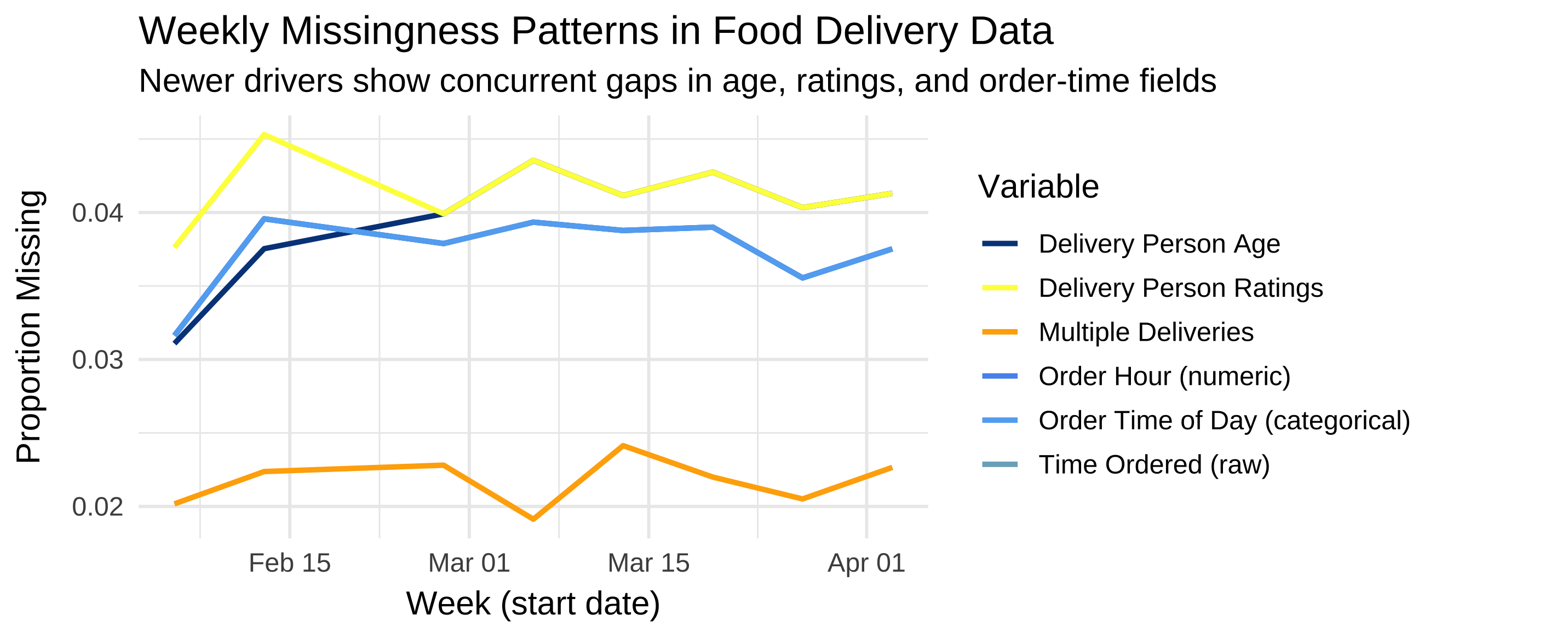
Let’s visualize how the proportion of missing values evolves weekly across all variables with known missingness.

# Summarize weekly missingness for all affected variables
df_summary <- food %>%
  mutate(
    week = floor_date(Order_Date, "week"),
    age_miss = is.na(Delivery_person_Age),
    rating_miss = is.na(Delivery_person_Ratings),
    multi_miss = is.na(multiple_deliveries),
    timeorder_miss = is.na(Time_Orderd),
    orderhour_miss = is.na(Order_Hour),
    ordertod_miss = is.na(Order_Time_of_Day)
  ) %>%
  group_by(week) %>%
  summarise(
    prop_age_miss = mean(age_miss, na.rm = TRUE),
    prop_rating_miss = mean(rating_miss, na.rm = TRUE),
    prop_multi_miss = mean(multi_miss, na.rm = TRUE),
    prop_timeorder_miss = mean(timeorder_miss, na.rm = TRUE),
    prop_orderhour_miss = mean(orderhour_miss, na.rm = TRUE),
    prop_ordertod_miss = mean(ordertod_miss, na.rm = TRUE),
    .groups = "drop"
  )

# Plot the weekly trends
df_summary %>%
  ggplot(aes(x = week)) +
  geom_line(aes(y = prop_age_miss, color = "Delivery Person Age"), linewidth = 1) +
  geom_line(aes(y = prop_rating_miss, color = "Delivery Person Ratings"), linewidth = 1) +
  geom_line(aes(y = prop_multi_miss, color = "Multiple Deliveries"), linewidth = 1) +
  geom_line(aes(y = prop_timeorder_miss, color = "Time Ordered (raw)"), linewidth = 1) +
  geom_line(aes(y = prop_orderhour_miss, color = "Order Hour (numeric)"), linewidth = 1) +
  geom_line(aes(y = prop_ordertod_miss, color = "Order Time of Day (categorical)"), linewidth = 1) +
  labs(
    title = "Weekly Missingness Patterns in Food Delivery Data",
    subtitle = "Newer drivers show concurrent gaps in age, ratings, and order-time fields",
    y = "Proportion Missing",
    x = "Week (start date)",
    color = "Variable"
  ) +
  theme_minimal(base_size = 13) +
  scale_color_manual(values = c(
    "Delivery Person Age" = "#044389",
    "Delivery Person Ratings" = "#FCFF4B",
    "Multiple Deliveries" = "#FFAD05",
    "Time Ordered (raw)" = "#7CAFC4",
    "Order Hour (numeric)" = "#5995ED",
    "Order Time of Day (categorical)" = "#63ADF2"
  ))

5.6.2 🔎 Confirming overlaps among derived time features

The three order-time variables (Time_Orderd, Order_Hour, and Order_Time_of_Day) perfectly overlap in the plot because they share identical missingness patterns. You can verify this directly from df_summary:

df_summary %>%
  summarise(
    same_time_vs_hour = all.equal(prop_timeorder_miss, prop_orderhour_miss),
    same_time_vs_tod  = all.equal(prop_timeorder_miss, prop_ordertod_miss),
    same_hour_vs_tod  = all.equal(prop_orderhour_miss, prop_ordertod_miss)
  )

Output:

# A tibble: 1 × 3
  same_time_vs_hour same_time_vs_tod same_hour_vs_tod
  <lgl>             <lgl>            <lgl>
1 TRUE              TRUE             TRUE

✅ This confirms that missing timestamps in Time_Orderd propagate exactly into Order_Hour and Order_Time_of_Day. In other words, these three lines are drawn on top of each other — the apparent “missing” lines are not lost, they’re simply perfectly coincident.

💡 Note: Overlapping lines as a sanity check

It’s normal to panic when you “lose” a line in a plot! But when multiple derived variables (like hour and day-part) are engineered from the same raw field, perfect overlap is actually a quality signal.

This overlap confirms that:

The transformation pipeline is consistent — missing raw timestamps produce missing derived values.
No artificial NAs or spurious imputations were introduced.
Downstream models will treat these three features as jointly missing, avoiding hidden bias.

So rather than a visualization bug, this is a quick sanity check for preprocessing integrity.

5.7 🔍 Key Insights

5.7.1 1. Shared missingness trend across multiple fields

All affected variables — Delivery_person_Age, Delivery_person_Ratings, multiple_deliveries, and the order-time variables — show parallel increases in missingness over time. This pattern rules out randomness → ❌ Not MCAR (Missing Completely at Random).

Interpretation: newer delivery drivers are being added to the system with incomplete profiles (no ratings, no age, no multiple-delivery records). The same growth trend is reflected in time-of-order fields — likely because timestamps were logged inconsistently for new users or incomplete transactions.

5.7.2 2. Consistent propagation of timestamp missingness

The three time-related variables (Time_Orderd, Order_Hour, and Order_Time_of_Day) mirror each other exactly, meaning missingness was faithfully propagated. Each missing timestamp produces missing derived values — this is expected and correct behavior.

This kind of alignment ensures feature engineering does not inadvertently “repair” missing data, which would otherwise lead to inconsistent or misleading downstream features.

5.7.3 3. `multiple_deliveries` has lower but correlated missingness

multiple_deliveries shows lower missingness overall, but its weekly pattern mirrors Delivery_person_Age and Delivery_person_Ratings. This implies it’s influenced by the same underlying process (new or unprofiled drivers). Lower missingness here is logical: the variable’s definition (“number of concurrent deliveries”) depends on operational events rather than profile completeness.

5.7.4 4. No Evidence of MNAR (Missing Not at Random)

We don’t see evidence that missingness depends on unobserved values — e.g., drivers with particularly low ratings being hidden or removed. The missingness correlates with observable temporal trends, not unmeasured traits.

This strongly supports a MAR (Missing At Random) process: missingness depends on observed data (such as time period or user onboarding), which we can explicitly model or handle with imputation methods like bagged trees.

5.8 🧠 Interpretation Summary

Mechanism	Definition	Typical Clues	Evidence in This Dataset	Conclusion
MCAR (Missing Completely at Random)	Data are missing independently of both observed and unobserved values.	Flat, random missingness across time and variables; no correlation with external patterns.	❌ Rejected — Missingness clearly increases over time and co-occurs across related variables (ratings, age, timestamps).	Not plausible; data collection changed systematically as new drivers entered.
MAR (Missing At Random)	Missingness depends on observed variables (e.g., time, onboarding stage).	Correlation between missingness and known, measurable processes.	✅ Strongly supported — Missing values cluster in newer weeks, indicating dependency on time and user experience.	Plausible; can be safely imputed using predictors such as date, city, or delivery density.
MNAR (Missing Not At Random)	Missingness depends on unobserved or hidden values (e.g., low-rated drivers avoid self-reporting).	Diverging trends, unexplained gaps, or missingness aligned with extreme predictor values.	⚠️ Unlikely — No divergence between variables, no hidden subgroups evident.	No direct evidence; could only be verified with external or longitudinal tracking data.

5.8.1 ✅ Summary Takeaway

The consistent, time-linked pattern of missing data across multiple variables strongly supports a MAR mechanism. This means the missingness process is explainable and can be handled safely with supervised imputation techniques (like bagged-tree imputation), which leverage other predictors without biasing model estimates.

The observed structure — where age, ratings, and order-time variables become missing together — suggests a single, operational cause: driver onboarding or delayed data entry.

5.9 Build a regression recipe

You will now create a recipe that predicts Time_taken(min) from reasonable predictors. Do not copy a pre-written recipe here — write your own using the tidymodels recipes reference: https://recipes.tidymodels.org/reference/index.html

Your recipe should:

Impute missing values with bagged trees (step_impute_bag()).
Convert categorical predictors to dummy variables (step_dummy()).
Normalize all numeric predictors (step_normalize()).
Remove zero-variance predictors (step_zv()).

5.9.1 ⚠️ Note on leakage

Always create and train your recipe after splitting the data. Defining the recipe is fine on the full dataset — it’s just a blueprint — but prep() must only ever be applied to the training data. tidymodels enforces this automatically when you put the recipe inside a workflow().

✅ One possible solution

cross_rec <- recipe(`Time_taken(min)` ~ ., data = cross_train) |>
  # Keep identifiers and raw geo/time fields OUT of the model:
  update_role(
    ID, Delivery_person_ID,
    Order_Date, Order_Week,          # keep for time-aware CV index, not as predictors
    Time_Orderd, Time_Order_picked,  # raw timestamps excluded, replaced by engineered features
    Restaurant_latitude, Restaurant_longitude,
    Delivery_location_latitude, Delivery_location_longitude,  # summarized by distance_km
    Season,                          # constant within one week → no info gain
    new_role = "ID"
  ) |>
  
  # Impute variables with known or propagated missingness using bagged trees
  step_impute_bag(
    all_of(c(
      "Delivery_person_Ratings", 
      "Delivery_person_Age", 
      "multiple_deliveries",
      "Order_Hour", 
      "Order_Time_of_Day"
    )),
    impute_with = imp_vars(all_predictors())
  ) |>
  
  # Convert categorical predictors (City, Traffic, Festival, etc.) to dummies
  step_dummy(all_nominal_predictors()) |>
  
  # Remove zero-variance columns
  step_zv(all_predictors()) |>
  
  # Normalize numeric predictors (optional for trees, but good general hygiene)
  step_normalize(all_numeric_predictors())

🔍 Recipe explanation (why each choice was made)

5.9.2 🧭 1. `update_role(...)`: protect non-predictors and avoid leakage

Some columns are essential for context and resampling, but would confuse or leak information if used as predictors:

Variable(s)	Why not a predictor?	New role
`ID`, `Delivery_person_ID`	Pure identifiers. They’d let the model memorize individuals rather than generalize patterns.	`"ID"`
`Order_Date`, `Order_Week`	Encode when an order occurred, not why it took longer. Including them risks temporal leakage. We keep them only to define time-aware CV later.	`"ID"`
`Time_Orderd`, `Time_Order_picked`	Raw timestamps are granular, cyclical, and sparse; we replaced them with the interpretable day-part features `Order_Time_of_Day` and `Time_of_Day`.	`"ID"`
`Restaurant_`, `Delivery_location_`	Separate lat/longs don’t express distance meaningfully and can mislead trees. We summarized them into `distance_km` using the Haversine formula.	`"ID"`
`Season`	In the cross-sectional subset (one week), `Season` has only one level → no variation → no signal. We’ll re-enable seasonality in the longitudinal analysis.	`"ID"`

Why “update role” instead of dropping?

We still need some fields for plots and time-aware resampling (e.g., Order_Date).
Keeping them documents the data lineage and makes the workflow reproducible and safe (no accidental reuse as predictors).

5.9.3 🧩 2. `step_impute_bag(...)`: principled missing-data handling

Bagged-tree imputation builds many small trees on bootstrap samples and averages their predictions for missing entries.
This preserves nonlinear relationships and interactions better than mean/mode imputation and is conceptually close to tree ensembles like Random Forests (variance reduction by averaging de-correlated trees).

💡 Note: Handling missingness in derived time features

Derived variables like Order_Hour and Order_Time_of_Day can be very predictive, but they inherit missingness from raw timestamps such as Time_Orderd.

By imputing them directly (and not the raw timestamp), we ensure that:

The model still benefits from time-of-day patterns,
Missingness is handled coherently across related variables, and
No data leakage occurs, since all imputations happen within training folds only.

This mirrors real-world modeling practice: engineer interpretable features → remove raw identifiers/timestamps → handle missingness at the feature level.

5.9.4 🧱 3. `step_dummy(all_nominal_predictors())`: turn categories into signals

Models need numeric inputs. This step converts text categories — e.g., City, Road_traffic_density, Festival, Type_of_order, Order_Time_of_Day, Time_of_Day — into 0/1 dummy columns.
Example: Time_of_Day = "Morning" becomes Time_of_Day_Morning = 1 for that row and 0 otherwise.

5.9.5 📏 4. `step_normalize(all_numeric_predictors())`: consistent scales

Some algorithms (KNN, SVM, penalized GLMs) are scale-sensitive.
Normalizing now keeps the recipe model-agnostic so students can swap models later without rewriting preprocessing.
Tree-based models are robust to scaling, so this step is harmless for LightGBM.

5.9.6 🧼 5. `step_zv(all_predictors())`: remove dead columns

After dummying and imputing, some columns may have zero variance. This step drops them to keep the model matrix clean.

5.10 Choose and specify a regression model – LightGBM

We will use LightGBM, a modern gradient-boosted-tree algorithm that is very efficient on large tabular data.

Both LightGBM and XGBoost implement gradient boosting: a sequence of small trees is trained, each correcting residual errors from previous trees. The difference lies in how they grow trees and manage splits:

XGBoost grows trees level-wise (balanced): it splits all leaves at one depth before going deeper. This produces symmetric trees and is often robust on small or moderately sized data.
LightGBM grows trees leaf-wise: it always expands the single leaf that most reduces the loss, yielding deeper, targeted trees. Together with histogram-based binning of features, this makes LightGBM faster and often stronger on large, sparse, or high-cardinality data.

5.10.1 Example specification

lgb_mod <- boost_tree(
  trees = 500,
  learn_rate = 0.1,
  tree_depth = 6,
  loss_reduction = 0.0,
  min_n = 2
) |>
  set_engine("lightgbm") |>
  set_mode("regression")

5.10.2 Common LightGBM tuning parameters

Parameter	What it controls	Intuition
`trees`	total number of trees	more trees can capture more structure but risk overfitting unless `learn_rate` is small
`learn_rate`	step size for each tree’s contribution	small = slower but safer learning; large = faster but riskier
`tree_depth`	maximum depth of a single tree	deeper trees capture complex interactions but can overfit
`loss_reduction`	minimum loss reduction to make a split	larger values prune weak splits and simplify trees
`min_n`	minimum observations in a leaf	prevents tiny leaves that memorize noise
`mtry`	number of predictors sampled at each split	adds randomness, reduces correlation among trees

When might you prefer XGBoost? On smaller datasets, when stability and interpretability matter. When might you prefer LightGBM? For speed on larger tables, many categorical dummies, or limited tuning time.

5.11 Combine recipe and model inside a workflow

Once your recipe and model specification are ready, combine them with workflow() so preprocessing and modeling stay linked. Workflows automatically apply the recipe before fitting or predicting.

reg_wf <- workflow() |>
  add_recipe(cross_rec) |>
  add_model(lgb_mod)

5.12 Evaluate the cross-sectional model

Fit your workflow on the training set and evaluate predictions on the test set.
Use regression metrics such as RMSE, MAE, and R².

🤺 Your turn

Compute and report these metrics for your model.
How accurate is the model on unseen data?
Does it tend to over- or under-predict delivery time?

✅ One possible solution

cross_fit <- reg_wf |> fit(cross_train)

cross_preds <- predict(cross_fit, cross_test) |>
  bind_cols(cross_test |> select(`Time_taken(min)`))

metric_set(rmse, mae, rsq)(
  cross_preds,
  truth = `Time_taken(min)`,
  estimate = .pred
)

Output

# A tibble: 3 × 3
  .metric .estimator .estimate
  <chr>   <chr>          <dbl>
1 rmse    standard       4.31 
2 mae     standard       3.43 
3 rsq     standard       0.771

💬 How to interpret these metrics

These results tell us that our model performs quite well for a single operational week — but with some natural limitations.

5.12.1 1️⃣ Accuracy of time predictions

An RMSE of about 4.3 minutes means that, on average, predicted delivery times are within roughly ±4–5 minutes of the actual values. Given that most deliveries take between 10 and 50 minutes, this error margin represents roughly 10–15% of a typical delivery duration — quite precise for a real-world logistics process.

The MAE of 3.4 minutes confirms that the typical prediction error is small and that the few large deviations (perhaps during peak traffic or bad weather) are not overwhelming. The gap between RMSE and MAE is modest, suggesting the model performs consistently across most deliveries, with only limited outlier impact.

5.12.2 2️⃣ How much variation the model explains

The R² value of 0.77 means that around three-quarters of all variation in delivery times can be explained by the predictors included — variables such as:

Distance, which captures spatial effort,
Traffic density, which captures congestion, and
Weather conditions, which influence travel safety and speed.

The remaining 23% of unexplained variation likely stems from unobserved or inherently random factors:

restaurant preparation times,
small detours or parking delays,
driver skill differences, or
special events not recorded in the dataset.

5.12.3 3️⃣ What this means in practice

For a restaurant manager or delivery company, this level of accuracy could already be useful:

Predicting when to alert customers (“your delivery will arrive in about 25 minutes”)
Planning driver assignments or restocking intervals
Identifying potential bottlenecks when actual times systematically exceed predictions

5.12.4 4️⃣ Important caveat: one week ≠ the whole story

Because this is a cross-sectional snapshot (one week only), the model hasn’t been tested on how patterns evolve over time. For example:

Festivals or new delivery routes might change the relationships between predictors and time,
Weather patterns might shift from winter to spring,
Or new drivers might behave differently from earlier ones.

Therefore, the next step — time-aware cross-validation — will tell us whether this model remains reliable when predicting future weeks rather than just this one.

🤔 Explore residuals: how well does your model really perform?

Numerical metrics tell part of the story — but to see how your model behaves, you need to inspect residuals (the differences between actual and predicted delivery times).

Try plotting:

Predicted vs. actual delivery times
→ Are most points near the diagonal (perfect predictions)?
→ Do errors grow with longer delivery times?
Residuals vs. predicted values
→ Are residuals centered around zero (no systematic bias)?
→ Do you see patterns that might suggest missing predictors?
Residuals by time of day
→ Are certain times (e.g., evening rush hours) consistently over- or under-predicted?

Write a short paragraph summarizing what you notice.
Does the model perform equally well for all deliveries, or does it struggle under specific conditions?

5.12.5 Cross-validation on the cross-sectional data

So far, you evaluated the model with a single train/test split. In a cross-sectional setting (no time ordering), it is common to use k-fold cross-validation, which splits the training data into k random folds, training on k – 1 folds and validating on the remaining fold in turn. This yields a more robust estimate of performance stability.

set.seed(42)
cv_cross <- vfold_cv(cross_train, v = 5)

cross_cv_res <- fit_resamples(
  reg_wf,
  resamples = cv_cross,
  metrics = metric_set(rmse, mae, rsq),
  control = control_resamples(save_pred = TRUE)
)

collect_metrics(cross_cv_res)

🤺 Your turn

Run a 5-fold cross-validation on the cross-sectional training data. Compare the average RMSE and R² to those from the single test-set evaluation. Are they similar? Which estimate do you trust more?

✅ One possible solution

Output

# A tibble: 3 × 6
  .metric .estimator  mean     n std_err .config        
  <chr>   <chr>      <dbl> <int>   <dbl> <chr>          
1 mae     standard   3.50      5 0.0235  pre0_mod0_post0
2 rmse    standard   4.51      5 0.0327  pre0_mod0_post0
3 rsq     standard   0.756     5 0.00324 pre0_mod0_post0

Interpretation:

The CV metrics are close to the single test-set values, confirming consistent performance. Cross-validation gives a more stable estimate because it reuses the data more efficiently.

5.13 Time-aware validation with `sliding_period()`

In time-dependent data, future information must not influence the model’s training. To mimic real-world deployment, we roll forward through time: train on past weeks, validate on the next week(s).

food <- food |>
  mutate(
    Season = case_when(
      Order_Week %in% 1:13   ~ "Winter",
      Order_Week %in% 14:26  ~ "Spring",
      Order_Week %in% 27:39  ~ "Summer",
      Order_Week %in% 40:52  ~ "Autumn",
      TRUE ~ NA_character_
    ),
    Season = factor(Season, levels = c("Winter", "Spring", "Summer", "Autumn"))
) #Season is converted to factor so that it's correctly handled by steps that require factor variables e.g step_novel() or step_dummy()
  
# create a chronological split first
set.seed(42)
long_split <- initial_time_split(food, prop = 0.8)
long_train <- training(long_split)
long_test  <- testing(long_split)

cv_long <- sliding_period(
  data        = long_train,  # your longitudinal training data (not the full dataset!)
  index       = Order_Date,
  period      = "week",
  lookback    = Inf,        # how many past weeks form the training window
  assess_stop = 1         # how many future weeks form the validation window
)

⚠️ Avoid leakage!

Never define cross-validation folds on the entire dataset. If you did, the model could “peek” at future data while training, inflating performance. Instead, use only the training portion of your longitudinal split—here called long_train.

5.13.1 How `sliding_period()` works

sliding_period() creates a sequence of rolling resamples ordered by the variable given in index. Here, the index is Order_Date, which is of class Date. Because it understands the class of this variable, rsample can interpret the keyword period = "week" as:

“Use the calendar weeks implied by the Date variable to move the window forward one week at a time.”

Internally, it uses date arithmetic (floor_date() and ceiling_date() logic) to determine where each new week starts and stops. If you had specified period = "day" or period = "month", it would instead roll forward daily or monthly. Thus, period defines the temporal granularity of each split, and index provides the timeline to follow.

Peering inside the cross-validation folds

Let’s try and have a look at which dates the sliding_period() cross-validation folds correspond to:

cv_long_summary <- cv_long %>%
  mutate(
    train_start = map(splits, ~ min(analysis(.x)$Order_Date)),
    train_end   = map(splits, ~ max(analysis(.x)$Order_Date)),
    val_start   = map(splits, ~ min(assessment(.x)$Order_Date)),
    val_end     = map(splits, ~ max(assessment(.x)$Order_Date))
  ) %>%
  tidyr::unnest(c(train_start, train_end, val_start, val_end)) %>%
  select(id, train_start, train_end, val_start, val_end)

cv_long_summary

# A tibble: 6 × 5
  id     train_start train_end  val_start  val_end   
  <chr>  <date>      <date>     <date>     <date>    
1 Slice1 2022-02-11  2022-02-16 2022-02-17 2022-02-18
2 Slice2 2022-02-11  2022-02-18 2022-03-01 2022-03-02
3 Slice3 2022-02-11  2022-03-02 2022-03-03 2022-03-09
4 Slice4 2022-02-11  2022-03-09 2022-03-10 2022-03-16
5 Slice5 2022-02-11  2022-03-16 2022-03-17 2022-03-23
6 Slice6 2022-02-11  2022-03-23 2022-03-24 2022-03-29

If you want to have a look at which weeks these folds correspond to instead:

cv_long_summary_weeks <- cv_long %>%
  mutate(
    train_start_wk = map_int(splits, ~ isoweek(min(analysis(.x)$Order_Date))),
    train_end_wk   = map_int(splits, ~ isoweek(max(analysis(.x)$Order_Date))),
    val_start_wk   = map_int(splits, ~ isoweek(min(assessment(.x)$Order_Date))),
    val_end_wk     = map_int(splits, ~ isoweek(max(assessment(.x)$Order_Date)))
  ) %>%
  select(id, train_start_wk, train_end_wk, val_start_wk, val_end_wk)

cv_long_summary_weeks

# A tibble: 6 × 5
  id     train_start_wk train_end_wk val_start_wk val_end_wk
  <chr>           <int>        <int>        <int>      <int>
1 Slice1              6            7            7          7
2 Slice2              6            7            9          9
3 Slice3              6            9            9         10
4 Slice4              6           10           10         11
5 Slice5              6           11           11         12
6 Slice6              6           12           12         13

And if you want to visualise the folds:

cv_long_summary %>%
  mutate(id = factor(id, levels = rev(id))) %>%  # reverse for readability
  ggplot() +
  geom_segment(aes(x = train_start, xend = train_end, y = id, yend = id),
               color = "#0072B2", linewidth = 3) +
  geom_segment(aes(x = val_start, xend = val_end, y = id, yend = id),
               color = "#E69F00", linewidth = 3) +
  labs(
    title = "Expanding Weekly Sliding-Period Cross-Validation",
    x = "Date", y = "Slice",
    caption = "Blue = training window, Orange = validation window"
  ) +
  theme_minimal(base_size = 13)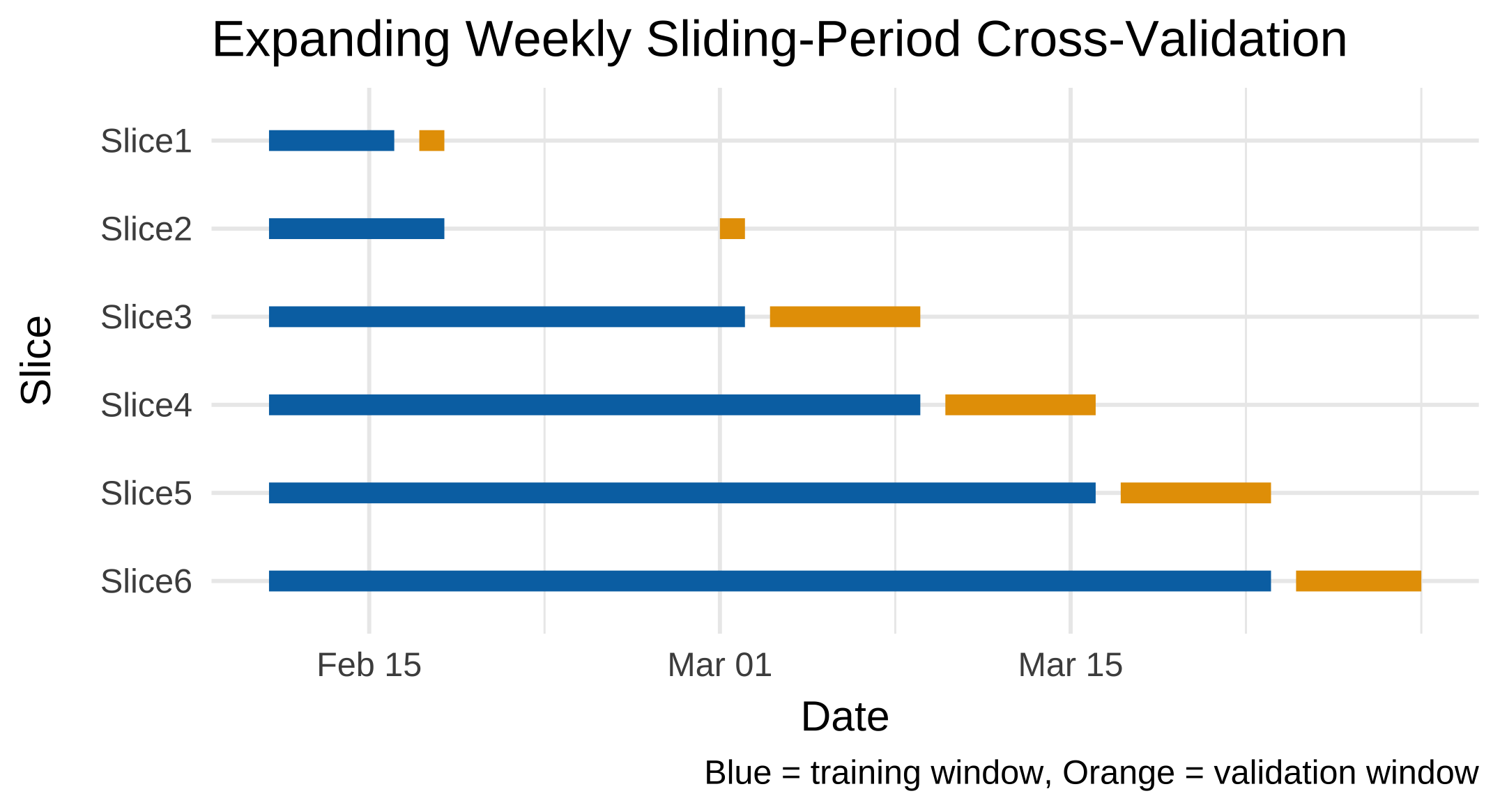

5.14 Recipe, workflow, and modeling for longitudinal validation

Repeat the full process—recipe, model, and workflow—on the longitudinal setup. Then train and evaluate the model using the time-aware resamples created above.

🤺 Your turn

Use fit_resamples() to fit your LightGBM workflow with cv_long. Collect metrics (rmse, mae, rsq) and summarize them.

✅ One possible solution

long_rec <- recipe(`Time_taken(min)` ~ ., data = long_train) |>
  # Exclude pure identifiers and raw time/geo columns from modeling
  update_role(
    ID, Delivery_person_ID,
    Order_Date, Order_Week,          # kept for time-aware resampling but not for prediction
    Time_Orderd, Time_Order_picked,  # raw timestamps replaced by engineered features
    Restaurant_latitude, Restaurant_longitude,
    Delivery_location_latitude, Delivery_location_longitude,
    new_role = "ID"
  ) |>
  # Impute missing values using bagged trees
  step_impute_bag(
    all_of(c(
      "Delivery_person_Ratings", 
      "Delivery_person_Age", 
      "multiple_deliveries",
      "Order_Hour",
      "Order_Time_of_Day"
    )),
    impute_with = imp_vars(all_predictors())
  ) |>
  # Handle unseen categorical levels (e.g., new "Spring" season appearing post-training)
  step_novel(all_nominal_predictors()) |>
  # Convert categorical predictors (Season, City, Road_traffic_density, Festival, etc.)
  step_dummy(all_nominal_predictors()) |>
  # Remove zero-variance columns
  step_zv(all_predictors()) |>
  # Normalize numeric predictors (safe default even for trees)
  step_normalize(all_numeric_predictors())

long_wf <- workflow() |>
  add_recipe(long_rec) |>
  add_model(lgb_mod)

set.seed(42)
long_res <- fit_resamples(
  long_wf,
  resamples = cv_long,
  metrics = metric_set(rmse, mae, rsq),
  control = control_resamples(save_pred = TRUE)
)

collect_metrics(long_res)

5.14.1 🧭 Explanation

5.14.1.1 1. Roles updated like the cross-sectional recipe

We exclude identifiers and raw geographic/time fields that could cause leakage or confuse the model. Unlike the cross-sectional version, we keep Season as a predictor now, because time variation matters in longitudinal modeling.

Variable(s)	Role	Why
`ID`, `Delivery_person_ID`	`"ID"`	Unique identifiers; would lead to memorization if used as predictors.
`Order_Date`, `Order_Week`	`"ID"`	Used only as the time index for resampling, not for prediction.
`Time_Orderd`, `Time_Order_picked`	`"ID"`	Replaced by derived variables (`Order_Hour`, `Order_Time_of_Day`, etc.) that capture interpretable cyclic patterns.
`Restaurant_latitude`/`longitude`, `Delivery_location_latitude`/`longitude`	`"ID"`	Represented more meaningfully by the engineered feature `distance_km`.

Season remains a predictor because it provides temporal context (seasonal traffic, weather, demand).

5.14.1.2 2. Imputation covers all known-missing columns

We explicitly include all variables where we’ve observed missingness:

Delivery_person_Ratings
Delivery_person_Age
multiple_deliveries
Order_Hour
Order_Time_of_Day

This ensures consistent treatment between short-term (cross-sectional) and longitudinal contexts.

5.14.1.3 3. `step_novel()` — essential for unseen levels

Because all training data belong to Winter but testing includes Spring deliveries, step_novel() is added before dummy encoding to handle new categorical levels gracefully.

Without it, bake() would fail when encountering "Spring", since the recipe prepared only "Winter". This step mimics real-world temporal generalization — when a model trained in one period faces new categories later.

5.14.1.4 4. Normalization kept for generality

Although tree-based models (like LightGBM) don’t require normalized inputs, this normalization step helps if you later try linear, ElasticNet, KNN or SVM models.

📚 Why align recipes across designs?

Using nearly identical recipes for cross-sectional and longitudinal designs:

Makes comparisons fair — differences in results reflect temporal validation, not preprocessing.
Ensures data preparation is stable across experiments (so that performance differences can be ascribed to modeling not data preparation!).
Simplifies later workflow assembly and hyperparameter tuning code.

🌦 Handling new seasonal categories

Because our longitudinal training data only include Winter deliveries, but the test data add Spring ones, the model will face an unseen category at prediction time.

step_novel() ensures the recipe anticipates new levels like "Spring" and assigns them to a safe “novel” category during encoding, avoiding model failure.

This is a real-world example of temporal covariate shift — new conditions (e.g., new seasons, new cities, or new delivery modes) appearing after training.

Output

# A tibble: 3 × 6
  .metric .estimator  mean     n std_err .config        
  <chr>   <chr>      <dbl> <int>   <dbl> <chr>          
1 mae     standard   3.30      6 0.0634  pre0_mod0_post0
2 rmse    standard   4.18      6 0.0813  pre0_mod0_post0
3 rsq     standard   0.797     6 0.00948 pre0_mod0_post0

Note: Expect slightly different numbers than the cross-sectional test split because (a) folds change over weeks, and (b) training windows grow over time.

5.15 Challenge: comparing designs

Compare your cross-sectional and longitudinal results.

💬 Think about this

Are the results directly comparable? Why or why not?
Which design better represents real-world performance, and why?
How does time-aware validation change your interpretation of model quality?

✅ One possible solution

5.15.1 🔍 Summary of results

Design	RMSE ↓	MAE ↓	R² ↑	Resampling	Notes
Cross-sectional (CV)	4.51	3.50	0.756	Random folds within one week	Easier problem — limited temporal drift
Longitudinal (rolling CV)	4.18	3.30	0.797	Past→Future expanding windows	Harder setup but more realistic

5.15.2 🧭 Interpretation

1. Are the results directly comparable?
Not entirely.
The cross-sectional design samples from a single busy week with random splits, while the longitudinal setup uses sequential, expanding windows across multiple weeks.
Each fold in the longitudinal setup reflects a different temporal context — so its performance better represents how a deployed model will behave as conditions evolve.

Moreover, the two designs differ in data distribution and training volume: the cross-sectional model sees only one high-stress operational regime (e.g., consistent traffic, weather, and driver behavior), whereas the longitudinal model trains on an accumulating history of weeks with varying conditions (festivals, weather shifts, new drivers). This means the longitudinal model benefits from more diverse and abundant training data, which can improve generalization. Because of these differences—distributional shift, temporal structure, and data volume—the metrics are not strictly comparable; they answer subtly different questions about model behavior.

2. Which design better represents real-world deployment?
The time-aware longitudinal design does.
In real applications, we predict future deliveries using patterns learned from the past — never mixing the two.
Its slightly lower RMSE and MAE combined with higher R² suggest that the model generalizes robustly across time, not just within one week’s context.

Critically, this design respects temporal causality: no future information leaks into training. Random cross-sectional CV violates this principle by shuffling observations across time, which inflates performance estimates and creates a false sense of reliability. The longitudinal approach, by contrast, simulates real forecasting conditions—making its results not only more realistic but also more trustworthy for operational planning. The larger standard errors in the longitudinal metrics (e.g., RMSE std_err = 0.081 vs. 0.033) further reflect the natural variability in delivery dynamics over time—a feature, not a bug, as it honestly quantifies uncertainty in a changing environment.

3. Why did the longitudinal model slightly outperform the cross-sectional one?
A few plausible reasons:

The longitudinal design uses more total training data (cumulative weeks), improving stability.
Seasonal/contextual predictors (e.g., traffic density, weather) add meaningful temporal variation.
The model may have learned smoother relationships by observing multiple weekly contexts.

Importantly, although time-aware validation is typically more challenging, here the benefit of richer, more varied training data appears to outweigh the difficulty of forecasting the future—leading to better overall performance.

4. Key takeaway
If a model performs consistently under time-aware validation, it is more trustworthy for forecasting tasks, even if cross-sectional metrics look similar or slightly better.
For any prediction task involving time, time-aware validation isn’t just preferable—it’s essential to avoid overestimating real-world performance and deploying models that fail when conditions evolve.

📏 Why we used cross-validation metrics here

In this tutorial, we compared cross-validation results (rather than test-set results) for a key reason:

Cross-validation gives a distribution of model performance across multiple folds (or time windows), revealing stability and temporal robustness. The test set, by contrast, is a single split — useful for final confirmation, but not sufficient to judge generalization on its own.

In time-aware setups, each resample already acts as a mini test, predicting unseen weeks from prior ones. Hence, cross-validation metrics are the most informative comparison across designs:

Cross-sectional CV: tests within one busy week (random 80/20)
Time-aware CV: tests repeatedly across future weeks (expanding window)

Later, we’ll complement these with final test-set results when comparing LightGBM and ElasticNet directly.

5.16 🧗 Challenge: try another model

Repeat the workflow using a different algorithm of your choice (for example, Elastic-Net, SVM, or KNN). Do not copy specifications here — consult lectures, 📚labs W02–W05, and the reading week homework for syntax, recommended preprocessing, and tuning guidance.

Evaluate the alternative model on both cross-sectional and time-aware folds and compare results.

💭 Reflection

Which model generalized best over time?
Did any model overfit when using random folds but degrade under time-aware validation?
Which preprocessing steps (such as normalization) were essential for your chosen model, and why?
Would your preferred model still perform well if new conditions appeared (e.g., “Summer” deliveries or new cities)?

5.16.1 💡 Example models (and specification)

Model	Formula	Engine	Notes
Elastic-Net	`linear_reg(penalty = tune(), mixture = tune())`	`"glmnet"`	Requires normalized inputs; interpretable; may underfit nonlinear effects.
SVM (RBF)	`svm_rbf(cost = tune(), rbf_sigma = tune())`	`"kernlab"`	Handles nonlinearities; benefits from scaling; can be slower on large data.
KNN	`nearest_neighbor(neighbors = tune())`	`"kknn"`	Very sensitive to normalization; local patterns may not generalize well over time.

In what follows, we’ll focus on ElasticNet to contrast a linear, interpretable model with the nonlinear, high-performance LightGBM.

5.17 🔁 Elastic Net regression – cross-sectional design

# Elastic Net specification
enet_mod <- linear_reg(
  penalty = tune(),   # overall regularization strength (λ)
  mixture = tune()    # 0 = ridge, 1 = lasso, in-between = elastic
) |>
  set_engine("glmnet")

# Use the same recipe as the cross-sectional model
cross_enet_rec <- cross_rec

# Combine into workflow
cross_enet_wf <- workflow() |>
  add_recipe(cross_enet_rec) |>
  add_model(enet_mod)

# Define a grid of λ and α values
enet_grid <- grid_regular(
  penalty(range = c(-3, 0)),  # λ ≈ 10⁻³ → 1
  mixture(range = c(0, 1)),   # ridge → lasso
  levels = 6
)

set.seed(42)
cross_enet_res <- tune_grid(
  cross_enet_wf,
  resamples = cv_cross,
  grid = enet_grid,
  metrics = metric_set(rmse, mae, rsq),
  control = control_grid(save_pred = TRUE)
)

print(collect_metrics(cross_enet_res),n=110)

# A tibble: 108 × 8
    penalty mixture .metric .estimator  mean     n  std_err .config         
      <dbl>   <dbl> <chr>   <chr>      <dbl> <int>    <dbl> <chr>           
  1 0.001       0   mae     standard   4.85      5 0.0381   pre0_mod01_post0
  2 0.001       0   rmse    standard   6.15      5 0.0258   pre0_mod01_post0
  3 0.001       0   rsq     standard   0.547     5 0.00277  pre0_mod01_post0
  4 0.001       0.2 mae     standard   4.85      5 0.0363   pre0_mod02_post0
  5 0.001       0.2 rmse    standard   6.14      5 0.0229   pre0_mod02_post0
  6 0.001       0.2 rsq     standard   0.548     5 0.00267  pre0_mod02_post0
  7 0.001       0.4 mae     standard   4.85      5 0.0363   pre0_mod03_post0
  8 0.001       0.4 rmse    standard   6.14      5 0.0229   pre0_mod03_post0
  9 0.001       0.4 rsq     standard   0.548     5 0.00267  pre0_mod03_post0
 10 0.001       0.6 mae     standard   4.84      5 0.0367   pre0_mod04_post0
 11 0.001       0.6 rmse    standard   6.14      5 0.0231   pre0_mod04_post0
 12 0.001       0.6 rsq     standard   0.548     5 0.00269  pre0_mod04_post0
 13 0.001       0.8 mae     standard   4.84      5 0.0368   pre0_mod05_post0
 14 0.001       0.8 rmse    standard   6.14      5 0.0232   pre0_mod05_post0
 15 0.001       0.8 rsq     standard   0.548     5 0.00270  pre0_mod05_post0
 16 0.001       1   mae     standard   4.85      5 0.0364   pre0_mod06_post0
 17 0.001       1   rmse    standard   6.14      5 0.0229   pre0_mod06_post0
 18 0.001       1   rsq     standard   0.548     5 0.00267  pre0_mod06_post0
 19 0.00398     0   mae     standard   4.85      5 0.0381   pre0_mod07_post0
 20 0.00398     0   rmse    standard   6.15      5 0.0258   pre0_mod07_post0
 21 0.00398     0   rsq     standard   0.547     5 0.00277  pre0_mod07_post0
 22 0.00398     0.2 mae     standard   4.85      5 0.0363   pre0_mod08_post0
 23 0.00398     0.2 rmse    standard   6.14      5 0.0229   pre0_mod08_post0
 24 0.00398     0.2 rsq     standard   0.548     5 0.00267  pre0_mod08_post0
 25 0.00398     0.4 mae     standard   4.84      5 0.0362   pre0_mod09_post0
 26 0.00398     0.4 rmse    standard   6.14      5 0.0230   pre0_mod09_post0
 27 0.00398     0.4 rsq     standard   0.548     5 0.00265  pre0_mod09_post0
 28 0.00398     0.6 mae     standard   4.84      5 0.0366   pre0_mod10_post0
 29 0.00398     0.6 rmse    standard   6.14      5 0.0233   pre0_mod10_post0
 30 0.00398     0.6 rsq     standard   0.548     5 0.00266  pre0_mod10_post0
 31 0.00398     0.8 mae     standard   4.84      5 0.0367   pre0_mod11_post0
 32 0.00398     0.8 rmse    standard   6.14      5 0.0235   pre0_mod11_post0
 33 0.00398     0.8 rsq     standard   0.548     5 0.00266  pre0_mod11_post0
 34 0.00398     1   mae     standard   4.84      5 0.0363   pre0_mod12_post0
 35 0.00398     1   rmse    standard   6.14      5 0.0234   pre0_mod12_post0
 36 0.00398     1   rsq     standard   0.548     5 0.00262  pre0_mod12_post0
 37 0.0158      0   mae     standard   4.85      5 0.0381   pre0_mod13_post0
 38 0.0158      0   rmse    standard   6.15      5 0.0258   pre0_mod13_post0
 39 0.0158      0   rsq     standard   0.547     5 0.00277  pre0_mod13_post0
 40 0.0158      0.2 mae     standard   4.84      5 0.0365   pre0_mod14_post0
 41 0.0158      0.2 rmse    standard   6.14      5 0.0236   pre0_mod14_post0
 42 0.0158      0.2 rsq     standard   0.548     5 0.00262  pre0_mod14_post0
 43 0.0158      0.4 mae     standard   4.84      5 0.0369   pre0_mod15_post0
 44 0.0158      0.4 rmse    standard   6.14      5 0.0242   pre0_mod15_post0
 45 0.0158      0.4 rsq     standard   0.548     5 0.00265  pre0_mod15_post0
 46 0.0158      0.6 mae     standard   4.84      5 0.0371   pre0_mod16_post0
 47 0.0158      0.6 rmse    standard   6.14      5 0.0242   pre0_mod16_post0
 48 0.0158      0.6 rsq     standard   0.548     5 0.00264  pre0_mod16_post0
 49 0.0158      0.8 mae     standard   4.84      5 0.0371   pre0_mod17_post0
 50 0.0158      0.8 rmse    standard   6.14      5 0.0242   pre0_mod17_post0
 51 0.0158      0.8 rsq     standard   0.548     5 0.00265  pre0_mod17_post0
 52 0.0158      1   mae     standard   4.84      5 0.0369   pre0_mod18_post0
 53 0.0158      1   rmse    standard   6.14      5 0.0242   pre0_mod18_post0
 54 0.0158      1   rsq     standard   0.548     5 0.00264  pre0_mod18_post0
 55 0.0631      0   mae     standard   4.85      5 0.0381   pre0_mod19_post0
 56 0.0631      0   rmse    standard   6.15      5 0.0258   pre0_mod19_post0
 57 0.0631      0   rsq     standard   0.547     5 0.00277  pre0_mod19_post0
 58 0.0631      0.2 mae     standard   4.84      5 0.0372   pre0_mod20_post0
 59 0.0631      0.2 rmse    standard   6.14      5 0.0244   pre0_mod20_post0
 60 0.0631      0.2 rsq     standard   0.548     5 0.00267  pre0_mod20_post0
 61 0.0631      0.4 mae     standard   4.84      5 0.0362   pre0_mod21_post0
 62 0.0631      0.4 rmse    standard   6.14      5 0.0245   pre0_mod21_post0
 63 0.0631      0.4 rsq     standard   0.547     5 0.00262  pre0_mod21_post0
 64 0.0631      0.6 mae     standard   4.84      5 0.0356   pre0_mod22_post0
 65 0.0631      0.6 rmse    standard   6.14      5 0.0245   pre0_mod22_post0
 66 0.0631      0.6 rsq     standard   0.547     5 0.00255  pre0_mod22_post0
 67 0.0631      0.8 mae     standard   4.84      5 0.0349   pre0_mod23_post0
 68 0.0631      0.8 rmse    standard   6.15      5 0.0245   pre0_mod23_post0
 69 0.0631      0.8 rsq     standard   0.546     5 0.00247  pre0_mod23_post0
 70 0.0631      1   mae     standard   4.85      5 0.0340   pre0_mod24_post0
 71 0.0631      1   rmse    standard   6.15      5 0.0244   pre0_mod24_post0
 72 0.0631      1   rsq     standard   0.546     5 0.00237  pre0_mod24_post0
 73 0.251       0   mae     standard   4.85      5 0.0381   pre0_mod25_post0
 74 0.251       0   rmse    standard   6.15      5 0.0258   pre0_mod25_post0
 75 0.251       0   rsq     standard   0.547     5 0.00277  pre0_mod25_post0
 76 0.251       0.2 mae     standard   4.86      5 0.0346   pre0_mod26_post0
 77 0.251       0.2 rmse    standard   6.16      5 0.0248   pre0_mod26_post0
 78 0.251       0.2 rsq     standard   0.545     5 0.00246  pre0_mod26_post0
 79 0.251       0.4 mae     standard   4.88      5 0.0335   pre0_mod27_post0
 80 0.251       0.4 rmse    standard   6.18      5 0.0247   pre0_mod27_post0
 81 0.251       0.4 rsq     standard   0.542     5 0.00209  pre0_mod27_post0
 82 0.251       0.6 mae     standard   4.90      5 0.0329   pre0_mod28_post0
 83 0.251       0.6 rmse    standard   6.21      5 0.0254   pre0_mod28_post0
 84 0.251       0.6 rsq     standard   0.538     5 0.00200  pre0_mod28_post0
 85 0.251       0.8 mae     standard   4.91      5 0.0339   pre0_mod29_post0
 86 0.251       0.8 rmse    standard   6.24      5 0.0264   pre0_mod29_post0
 87 0.251       0.8 rsq     standard   0.536     5 0.00180  pre0_mod29_post0
 88 0.251       1   mae     standard   4.93      5 0.0344   pre0_mod30_post0
 89 0.251       1   rmse    standard   6.26      5 0.0276   pre0_mod30_post0
 90 0.251       1   rsq     standard   0.534     5 0.00170  pre0_mod30_post0
 91 1           0   mae     standard   4.88      5 0.0389   pre0_mod31_post0
 92 1           0   rmse    standard   6.18      5 0.0276   pre0_mod31_post0
 93 1           0   rsq     standard   0.543     5 0.00282  pre0_mod31_post0
 94 1           0.2 mae     standard   4.95      5 0.0374   pre0_mod32_post0
 95 1           0.2 rmse    standard   6.27      5 0.0286   pre0_mod32_post0
 96 1           0.2 rsq     standard   0.535     5 0.00194  pre0_mod32_post0
 97 1           0.4 mae     standard   5.02      5 0.0393   pre0_mod33_post0
 98 1           0.4 rmse    standard   6.36      5 0.0343   pre0_mod33_post0
 99 1           0.4 rsq     standard   0.531     5 0.00107  pre0_mod33_post0
100 1           0.6 mae     standard   5.12      5 0.0423   pre0_mod34_post0
101 1           0.6 rmse    standard   6.49      5 0.0401   pre0_mod34_post0
102 1           0.6 rsq     standard   0.524     5 0.000917 pre0_mod34_post0
103 1           0.8 mae     standard   5.24      5 0.0428   pre0_mod35_post0
104 1           0.8 rmse    standard   6.63      5 0.0441   pre0_mod35_post0
105 1           0.8 rsq     standard   0.516     5 0.00127  pre0_mod35_post0
106 1           1   mae     standard   5.39      5 0.0403   pre0_mod36_post0
107 1           1   rmse    standard   6.79      5 0.0447   pre0_mod36_post0
108 1           1   rsq     standard   0.508     5 0.00157  pre0_mod36_post0

📈 Tuning outcome summary

The Elastic Net grid search produced remarkably stable results across all combinations of the penalty (λ) and mixture (α) parameters. Neither stronger regularization nor changes in the ridge–lasso balance materially affected model performance:

Metric	Mean ± SE	Interpretation
RMSE	6.14 ± 0.03	Prediction error varied by less than 0.05 minutes across the grid → very flat error surface.
MAE	4.85 ± 0.04	Small, stable deviations across folds → regularization strength has minimal effect.
R²	0.55 ± 0.01	Indicates that only about half of the variation in delivery time is captured by a linear additive structure.

Interpretation:

This tuning profile suggests that the Elastic Net model is insensitive to the regularization path—a hallmark of data where predictors are moderately collinear but relationships remain roughly linear. The flat performance landscape implies that most signal is already being captured by the baseline linear combination of features, with no further benefit from shrinking or sparsifying coefficients.

However, the limited (R^2 ) also reveals that a substantial nonlinear or interaction component remains unexplained. These are precisely the kinds of effects that tree-based ensembles (like LightGBM) can exploit—non-additive interactions between distance, traffic density, and time of day that a linear model cannot represent.

Takeaway: Elastic Net yields a stable but constrained fit—ideal for interpretability and diagnostic insight, but not for squeezing out the last increments of predictive accuracy. Its near-ridge behaviour (best λ ≈ 0.001, α ≈ 0.4–0.6) further confirms that the model benefits from mild shrinkage rather than sparsity.

5.18 ⏳ Elastic Net regression – longitudinal (time-aware) design

# Use the same recipe as the longitudinal model
long_enet_rec <- long_rec

long_enet_wf <- workflow() |>
  add_recipe(long_enet_rec) |>
  add_model(enet_mod)

set.seed(42)
long_enet_res <- tune_grid(
  long_enet_wf,
  resamples = cv_long,
  grid = enet_grid,
  metrics = metric_set(rmse, mae, rsq),
  control = control_grid(save_pred = TRUE)
)

print(collect_metrics(long_enet_res),n=110)

# A tibble: 108 × 8
    penalty mixture .metric .estimator  mean     n std_err .config         
      <dbl>   <dbl> <chr>   <chr>      <dbl> <int>   <dbl> <chr>           
  1 0.001       0   mae     standard   4.88      6 0.0418  pre0_mod01_post0
  2 0.001       0   rmse    standard   6.17      6 0.0567  pre0_mod01_post0
  3 0.001       0   rsq     standard   0.561     6 0.00731 pre0_mod01_post0
  4 0.001       0.2 mae     standard   4.87      6 0.0407  pre0_mod02_post0
  5 0.001       0.2 rmse    standard   6.15      6 0.0561  pre0_mod02_post0
  6 0.001       0.2 rsq     standard   0.563     6 0.00753 pre0_mod02_post0
  7 0.001       0.4 mae     standard   4.87      6 0.0409  pre0_mod03_post0
  8 0.001       0.4 rmse    standard   6.15      6 0.0563  pre0_mod03_post0
  9 0.001       0.4 rsq     standard   0.563     6 0.00753 pre0_mod03_post0
 10 0.001       0.6 mae     standard   4.87      6 0.0408  pre0_mod04_post0
 11 0.001       0.6 rmse    standard   6.15      6 0.0561  pre0_mod04_post0
 12 0.001       0.6 rsq     standard   0.564     6 0.00753 pre0_mod04_post0
 13 0.001       0.8 mae     standard   4.87      6 0.0407  pre0_mod05_post0
 14 0.001       0.8 rmse    standard   6.15      6 0.0561  pre0_mod05_post0
 15 0.001       0.8 rsq     standard   0.563     6 0.00752 pre0_mod05_post0
 16 0.001       1   mae     standard   4.87      6 0.0407  pre0_mod06_post0
 17 0.001       1   rmse    standard   6.15      6 0.0561  pre0_mod06_post0
 18 0.001       1   rsq     standard   0.563     6 0.00752 pre0_mod06_post0
 19 0.00398     0   mae     standard   4.88      6 0.0418  pre0_mod07_post0
 20 0.00398     0   rmse    standard   6.17      6 0.0567  pre0_mod07_post0
 21 0.00398     0   rsq     standard   0.561     6 0.00731 pre0_mod07_post0
 22 0.00398     0.2 mae     standard   4.87      6 0.0407  pre0_mod08_post0
 23 0.00398     0.2 rmse    standard   6.15      6 0.0562  pre0_mod08_post0
 24 0.00398     0.2 rsq     standard   0.563     6 0.00753 pre0_mod08_post0
 25 0.00398     0.4 mae     standard   4.87      6 0.0410  pre0_mod09_post0
 26 0.00398     0.4 rmse    standard   6.15      6 0.0564  pre0_mod09_post0
 27 0.00398     0.4 rsq     standard   0.563     6 0.00753 pre0_mod09_post0
 28 0.00398     0.6 mae     standard   4.87      6 0.0409  pre0_mod10_post0
 29 0.00398     0.6 rmse    standard   6.15      6 0.0564  pre0_mod10_post0
 30 0.00398     0.6 rsq     standard   0.563     6 0.00751 pre0_mod10_post0
 31 0.00398     0.8 mae     standard   4.87      6 0.0408  pre0_mod11_post0
 32 0.00398     0.8 rmse    standard   6.15      6 0.0564  pre0_mod11_post0
 33 0.00398     0.8 rsq     standard   0.563     6 0.00750 pre0_mod11_post0
 34 0.00398     1   mae     standard   4.87      6 0.0409  pre0_mod12_post0
 35 0.00398     1   rmse    standard   6.15      6 0.0565  pre0_mod12_post0
 36 0.00398     1   rsq     standard   0.563     6 0.00749 pre0_mod12_post0
 37 0.0158      0   mae     standard   4.88      6 0.0418  pre0_mod13_post0
 38 0.0158      0   rmse    standard   6.17      6 0.0567  pre0_mod13_post0
 39 0.0158      0   rsq     standard   0.561     6 0.00731 pre0_mod13_post0
 40 0.0158      0.2 mae     standard   4.87      6 0.0410  pre0_mod14_post0
 41 0.0158      0.2 rmse    standard   6.15      6 0.0566  pre0_mod14_post0
 42 0.0158      0.2 rsq     standard   0.563     6 0.00747 pre0_mod14_post0
 43 0.0158      0.4 mae     standard   4.87      6 0.0414  pre0_mod15_post0
 44 0.0158      0.4 rmse    standard   6.15      6 0.0571  pre0_mod15_post0
 45 0.0158      0.4 rsq     standard   0.563     6 0.00743 pre0_mod15_post0
 46 0.0158      0.6 mae     standard   4.87      6 0.0417  pre0_mod16_post0
 47 0.0158      0.6 rmse    standard   6.15      6 0.0573  pre0_mod16_post0
 48 0.0158      0.6 rsq     standard   0.563     6 0.00740 pre0_mod16_post0
 49 0.0158      0.8 mae     standard   4.87      6 0.0422  pre0_mod17_post0
 50 0.0158      0.8 rmse    standard   6.16      6 0.0575  pre0_mod17_post0
 51 0.0158      0.8 rsq     standard   0.562     6 0.00736 pre0_mod17_post0
 52 0.0158      1   mae     standard   4.87      6 0.0425  pre0_mod18_post0
 53 0.0158      1   rmse    standard   6.16      6 0.0577  pre0_mod18_post0
 54 0.0158      1   rsq     standard   0.562     6 0.00731 pre0_mod18_post0
 55 0.0631      0   mae     standard   4.88      6 0.0418  pre0_mod19_post0
 56 0.0631      0   rmse    standard   6.17      6 0.0567  pre0_mod19_post0
 57 0.0631      0   rsq     standard   0.561     6 0.00731 pre0_mod19_post0
 58 0.0631      0.2 mae     standard   4.87      6 0.0426  pre0_mod20_post0
 59 0.0631      0.2 rmse    standard   6.16      6 0.0576  pre0_mod20_post0
 60 0.0631      0.2 rsq     standard   0.562     6 0.00733 pre0_mod20_post0
 61 0.0631      0.4 mae     standard   4.87      6 0.0434  pre0_mod21_post0
 62 0.0631      0.4 rmse    standard   6.16      6 0.0581  pre0_mod21_post0
 63 0.0631      0.4 rsq     standard   0.562     6 0.00733 pre0_mod21_post0
 64 0.0631      0.6 mae     standard   4.87      6 0.0432  pre0_mod22_post0
 65 0.0631      0.6 rmse    standard   6.16      6 0.0583  pre0_mod22_post0
 66 0.0631      0.6 rsq     standard   0.562     6 0.00729 pre0_mod22_post0
 67 0.0631      0.8 mae     standard   4.87      6 0.0429  pre0_mod23_post0
 68 0.0631      0.8 rmse    standard   6.17      6 0.0582  pre0_mod23_post0
 69 0.0631      0.8 rsq     standard   0.561     6 0.00725 pre0_mod23_post0
 70 0.0631      1   mae     standard   4.88      6 0.0426  pre0_mod24_post0
 71 0.0631      1   rmse    standard   6.17      6 0.0581  pre0_mod24_post0
 72 0.0631      1   rsq     standard   0.560     6 0.00719 pre0_mod24_post0
 73 0.251       0   mae     standard   4.88      6 0.0418  pre0_mod25_post0
 74 0.251       0   rmse    standard   6.17      6 0.0567  pre0_mod25_post0
 75 0.251       0   rsq     standard   0.561     6 0.00731 pre0_mod25_post0
 76 0.251       0.2 mae     standard   4.89      6 0.0424  pre0_mod26_post0
 77 0.251       0.2 rmse    standard   6.18      6 0.0577  pre0_mod26_post0
 78 0.251       0.2 rsq     standard   0.559     6 0.00720 pre0_mod26_post0
 79 0.251       0.4 mae     standard   4.91      6 0.0425  pre0_mod27_post0
 80 0.251       0.4 rmse    standard   6.20      6 0.0582  pre0_mod27_post0
 81 0.251       0.4 rsq     standard   0.556     6 0.00707 pre0_mod27_post0
 82 0.251       0.6 mae     standard   4.92      6 0.0434  pre0_mod28_post0
 83 0.251       0.6 rmse    standard   6.23      6 0.0598  pre0_mod28_post0
 84 0.251       0.6 rsq     standard   0.554     6 0.00691 pre0_mod28_post0
 85 0.251       0.8 mae     standard   4.94      6 0.0443  pre0_mod29_post0
 86 0.251       0.8 rmse    standard   6.25      6 0.0612  pre0_mod29_post0
 87 0.251       0.8 rsq     standard   0.551     6 0.00686 pre0_mod29_post0
 88 0.251       1   mae     standard   4.96      6 0.0453  pre0_mod30_post0
 89 0.251       1   rmse    standard   6.28      6 0.0626  pre0_mod30_post0
 90 0.251       1   rsq     standard   0.549     6 0.00674 pre0_mod30_post0
 91 1           0   mae     standard   4.91      6 0.0418  pre0_mod31_post0
 92 1           0   rmse    standard   6.21      6 0.0558  pre0_mod31_post0
 93 1           0   rsq     standard   0.556     6 0.00715 pre0_mod31_post0
 94 1           0.2 mae     standard   4.98      6 0.0460  pre0_mod32_post0
 95 1           0.2 rmse    standard   6.29      6 0.0610  pre0_mod32_post0
 96 1           0.2 rsq     standard   0.549     6 0.00677 pre0_mod32_post0
 97 1           0.4 mae     standard   5.07      6 0.0460  pre0_mod33_post0
 98 1           0.4 rmse    standard   6.40      6 0.0618  pre0_mod33_post0
 99 1           0.4 rsq     standard   0.541     6 0.00656 pre0_mod33_post0
100 1           0.6 mae     standard   5.16      6 0.0480  pre0_mod34_post0
101 1           0.6 rmse    standard   6.52      6 0.0654  pre0_mod34_post0
102 1           0.6 rsq     standard   0.536     6 0.00666 pre0_mod34_post0
103 1           0.8 mae     standard   5.28      6 0.0522  pre0_mod35_post0
104 1           0.8 rmse    standard   6.66      6 0.0705  pre0_mod35_post0
105 1           0.8 rsq     standard   0.528     6 0.00668 pre0_mod35_post0
106 1           1   mae     standard   5.42      6 0.0546  pre0_mod36_post0
107 1           1   rmse    standard   6.82      6 0.0729  pre0_mod36_post0
108 1           1   rsq     standard   0.519     6 0.00646 pre0_mod36_post0

📈 Tuning outcome summary (time-aware design)

The Elastic Net tuning results under longitudinal (time-aware) cross-validation show a very similar pattern to the cross-sectional case: model performance remains stable across all tested penalty (λ) and mixture (α) values, confirming that regularization strength and sparsity weighting have little influence on predictive accuracy.

Metric	Mean ± SE	Interpretation
RMSE	6.16 ± 0.06	Virtually identical across grid; the model’s predictive surface is flat with respect to both λ and α.
MAE	4.88 ± 0.04	Stable and slightly lower than in the cross-sectional design → a modest gain in calibration over time.
R²	0.56 ± 0.01	Explains just over half of the variance in delivery time, marginally higher than before (≈ +0.01).

Interpretation. The near-constant error across the grid again points to ridge-like behaviour (α ≈ 0.4–0.6) where most coefficients are retained with mild shrinkage. Temporal resampling does not destabilize the model: each week’s validation error remains consistent, suggesting that the linear relationships between predictors and delivery time are stationary over the observation period.

The small R² improvement (0.56 vs 0.55) indicates that adding temporal diversity—training on cumulative past weeks—helps the model generalize slightly better, but the fundamental linear constraint remains. In other words, ElasticNet continues to model only average effects (e.g., “more distance → longer time”) and cannot capture changing slopes or nonlinearities like rush-hour congestion curves or interaction between traffic and city zone.

Takeaway: While LightGBM adapts flexibly to temporal shifts and complex feature interactions, ElasticNet serves as a robust baseline—its performance is consistent, reproducible, and largely unaffected by time-aware sampling. It provides a transparent benchmark for how much of the delivery-time variability can be explained by linear signal alone.

5.19 Selecting the best models

# Best ElasticNet model
best_enet <- select_best(long_enet_res, metric = "rmse")  # <-- named argument fix
# Best LIghtGBM model
best_lgb <- select_best(long_res, metric = "rmse")  # same fix here

5.20 🏁 Comparison of finalized models

To ensure a fair comparison, we refit both models with their best tuned parameters and evaluate them on the same test set.

# --- Elastic Net test evaluation ---
enet_preds <- predict(enet_final, long_test) |>
  bind_cols(long_test %>% select(`Time_taken(min)`))

enet_metrics <- enet_preds |>
  metrics(truth = `Time_taken(min)`, estimate = .pred) |>
  mutate(model = "Elastic Net")

# --- LightGBM test evaluation ---
lgb_preds <- predict(lgb_final, long_test) |>
  bind_cols(long_test %>% select(`Time_taken(min)`))

lgb_metrics <- lgb_preds |>
  metrics(truth = `Time_taken(min)`, estimate = .pred) |>
  mutate(model = "LightGBM")

# Combine with model names
test_comparison <- bind_rows(
  lgb_metrics,
  enet_metrics
) |>
  relocate(model, .before = .metric)

test_comparison

Output

# A tibble: 6 × 4
  model       .metric .estimator .estimate
  <chr>       <chr>   <chr>          <dbl>
1 LightGBM    rmse    standard       3.99 
2 LightGBM    rsq     standard       0.821
3 LightGBM    mae     standard       3.19 
4 Elastic Net rmse    standard       6.14 
5 Elastic Net rsq     standard       0.577
6 Elastic Net mae     standard       4.87

What does it tell us

This comparison shows that LightGBM is substantially better than Elastic Net at predicting food delivery times in our dataset. Here’s how to interpret each metric in context:

5.20.1 🚀 Key Takeaways

LightGBM reduces prediction error by ~35% (MAE: 3.19 vs 4.87 minutes).
It explains 82% of the variance in delivery times vs. 58% for Elastic Net.
The average prediction is within ~4 minutes of the true time (LightGBM RMSE), vs ~6 minutes for Elastic Net.

Given that delivery time is likely in the 10–50 minute range (based on typical food delivery), these differences are operationally significant.

5.20.2 🔍 Metric-by-Metric Interpretation

5.20.2.1 1. RMSE (Root Mean Squared Error)

LightGBM: 3.99 minutes
Elastic Net: 6.14 minutes
Interpretation:
RMSE penalizes larger errors more heavily. LightGBM’s lower RMSE means it avoids large misses (e.g., predicting 20 minutes when actual is 35). This is critical for customer satisfaction—nobody minds a slightly early delivery, but a 15-minute late one causes complaints.

5.20.2.2 2. MAE (Mean Absolute Error)

LightGBM: 3.19 minutes
Elastic Net: 4.87 minutes
Interpretation:
On average, LightGBM’s predictions are ~1.7 minutes closer to the true delivery time. In business terms: if you promise “30-minute delivery”, LightGBM ensures you meet that promise far more reliably.

5.20.2.3 3. R² (Coefficient of Determination)

LightGBM: 0.821
Elastic Net: 0.577
Interpretation:
LightGBM explains 82% of the variability in delivery times using your features (season, traffic, weather, etc.). Elastic Net only explains 58%, meaning it misses important patterns—likely non-linear effects (e.g., “Jam” traffic density having a disproportionate impact) or interactions (e.g., “Night + Urban + Festival = much slower”).

5.20.3 🤔 Why is LightGBM so much better?

Your features include:

Categorical variables with complex effects (City, Weatherconditions, Traffic)
Temporal patterns (Season, Time_of_Day)
Derived spatial features (distance_km)

Elastic Net assumes:

Linear relationships
Additive effects
No feature interactions (unless manually engineered)

LightGBM automatically captures:

Non-linearities (e.g., delivery time spikes during “Jam” traffic)
Interactions (e.g., scooters slow down more than motorcycles in rain)
Hierarchical patterns (e.g., urban vs. metropolitan behave differently by season)

This explains the large performance gap.

5.20.4 💡 Business Implications

Metric	LightGBM Benefit
MAE ↓ 35%	Fewer customer complaints about late deliveries
RMSE ↓ 35%	More reliable SLA (Service Level Agreement) adherence
R² ↑ 24 pts	Greater trust in delivery ETAs shown to customers in the app

We could even reduce buffer time in delivery promises (e.g., from “30–40 min” to “25–35 min”) using LightGBM’s more accurate predictions—improving competitiveness.

5.20.5 ⚠️ Caveat

We need to ensure this performance holds on truly future data (our time-based split already helps!)
We need to monitor for concept drift (e.g., new vehicle types, city expansions)

But as of now: we can deploy LightGBM. It’s clearly the superior model for this problem.

5.21 🔍 Comparing coefficients and feature importance

ElasticNet yields interpretable coefficients; LightGBM provides feature importances. Plotting them side-by-side shows how the two models “see” the data differently.

# --- 1️⃣ Elastic Net coefficients (from best tuned model)
coef_df <- tidy(enet_final) |>
  filter(term != "(Intercept)") |>
  arrange(desc(abs(estimate)))

coef_df %>%
  slice_head(n = 15) %>%
  ggplot(aes(x = reorder(term, abs(estimate)), y = estimate)) +
  geom_col(fill = "#56B4E9") +
  coord_flip() +
  labs(
    title = "Top Elastic-Net Coefficients (Longitudinal Model)",
    x = "Predictor",
    y = "Coefficient"
  ) +
  theme_minimal()

# --- 2️⃣ LightGBM feature importance (from previous workflow)
lgb_importance <- lgb_final |>
  extract_fit_parsnip() |>
  vip::vi()

vip::vip(lgb_importance, num_features = 15, geom = "col",
          aesthetics = list(fill = "#E69F00")) +
  labs(title = "Top LightGBM Feature Importances (Longitudinal Model)")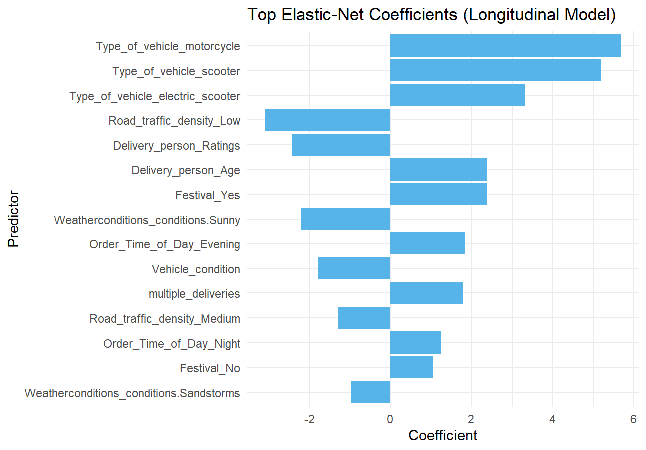

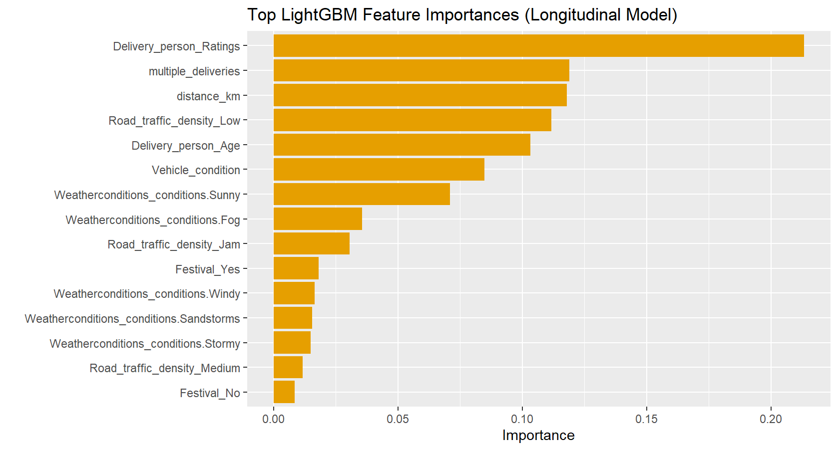
5.21.1 Interpretation

These two plots — LightGBM Feature Importance and Elastic Net Coefficients — give us complementary but very different insights into how each model “thinks” about delivery time prediction. Let’s break them down side-by-side.

5.21.1.1 🧭 1. LightGBM Feature Importance (Top 15)

“Which features does the tree-based model use most often to make splits?”

5.21.1.1.1 🔍 Key Observations:

Delivery_person_Ratings is #1 by a wide margin → This suggests that driver skill/experience (as captured by ratings) is the single strongest predictor of delivery speed.
multiple_deliveries and distance_km are #2 and #3 → Confirms intuition: more deliveries per trip = slower; longer distance = slower.
Road_traffic_density_Low is high → Low traffic helps, but note: “Jam” and “Medium” appear lower, meaning high traffic doesn’t dominate as much as low traffic helps (possibly because “Low” is common and has a strong positive effect).
Delivery_person_Age and Vehicle_condition matter → Older drivers or older vehicles may be slower.
Weather matters, but less than expected:
- Sunny > Fog > Windy, Sandstorms, Stormy
- Interestingly, no weather condition dominates — they’re all relatively low importance compared to driver ratings or distance.
Festival_Yes > Festival_No → Festivals slow things down (positive coefficient in Elastic Net too), but not as critical as core operational factors.

✅ Interpretation:
LightGBM prioritizes operational efficiency (driver quality, distance, load) over environmental conditions. It also captures non-linear and interaction effects implicitly — e.g., maybe “low traffic + sunny + young driver” is ultra-fast, but no single variable explains it alone.

5.21.1.2 📐 2. Elastic Net Coefficients (Top 15)

“What’s the linear effect of each feature on delivery time (after standardization)?”

5.21.1.2.1 🔍 Key Observations:

Type_of_vehicle_motorcycle and scooter have large positive coefficients → Wait, this seems counterintuitive? Actually, this likely means these are reference levels.
- In dummy encoding, if motorcycle is the baseline (omitted), then Type_of_vehicle_scooter = +5.0 means scooters take ~5 minutes longer than motorcycles.
- Similarly, electric_scooter = +3.5 → slower than motorcycle.
- So: Motorcycles are fastest, then electric scooters, then scooters.
Road_traffic_density_Low has a negative coefficient → Good! Lower traffic = faster delivery. Makes sense.
Delivery_person_Ratings has a negative coefficient → Higher ratings = faster delivery. Logical.
Festival_Yes is positive → Festivals increase delivery time (by ~2–3 minutes).
Order_Time_of_Day_Evening and Night are positive → Later orders take longer.
Weatherconditions_conditions.Sunny is negative → Sunny weather helps (faster delivery).
multiple_deliveries is positive → More deliveries = slower.
Festival_No is small and negative → Suggests “No Festival” is slightly better than baseline (but since “Yes” is positive, this reinforces festival = slowdown).

⚠️ Important Caveat:

Elastic Net coefficients are standardized, so they reflect relative impact after scaling. But because Elastic Net is linear, it misses interactions — e.g., it can’t say “Sunny + Low Traffic = super fast”, only “Sunny helps a little, Low Traffic helps a little”.

5.22 ⚖️ Side-by-Side Comparison: Why LightGBM Outperforms

Aspect	LightGBM	Elastic Net
Top Feature	Delivery_person_Ratings	Type_of_vehicle_motorcycle (baseline)
Model Type	Non-linear, tree-based	Linear, additive
Captures Interactions	✅ Yes (implicitly)	❌ No (unless manually engineered)
Handles Categoricals	✅ Naturally via splits	❌ Requires dummy encoding
Interpretability	Feature importance (global)	Coefficients (linear effect)
Why Better Here?	Captures complex real-world patterns	Oversimplifies relationships

5.23 💡 Business & Operational Insights

5.23.1 From LightGBM:

Invest in driver training/retention — High-rated drivers are your biggest asset.
Optimize multi-stop routes — Each extra delivery adds meaningful time.
Prioritize short-distance orders — Distance is a major cost driver.
Traffic density matters, but not as much as driver quality — Maybe invest in routing tech over traffic prediction.

5.23.2 From Elastic Net:

Motorcycles are fastest → Prioritize assigning them for urgent/short trips.
Festivals add ~2–3 minutes → Build buffer time during events.
Evening/Night orders take longer → Adjust ETAs dynamically.
Sunny weather helps — Consider offering discounts or promotions on sunny days to boost volume without hurting SLA.

5.24 🎯 Final Takeaway

LightGBM wins because it captures the messy, non-linear reality of food delivery.
Elastic Net gives you interpretable linear effects — useful for quick diagnostics — but misses the bigger picture.

Use LightGBM for prediction, and Elastic Net coefficients for initial feature understanding or regulatory reporting (where linearity and interpretability are required).

And if you want to explain why LightGBM predicts what it does, consider using SHAP values(Lundberg and Lee 2017) next — they’ll show you exactly how each feature contributes to each individual prediction.

5.24.1 📈 Synthesis Plot

cv_summary <- tibble::tribble(
  ~Model,        ~Design,             ~RMSE, ~MAE, ~R2,
  "LightGBM",    "Cross-sectional",   4.51,  3.50, 0.756,
  "LightGBM",    "Time-aware (CV)",   4.18,  3.30, 0.797,
  "LightGBM",    "Test set",          3.99,  3.19, 0.821,
  "ElasticNet",  "Cross-sectional",   6.14,  4.84, 0.548,
  "ElasticNet",  "Time-aware (CV)",   6.15,  4.87, 0.564,
  "ElasticNet",  "Test set",          6.14,  4.87, 0.577
)

# Pivot longer: one row per metric
cv_long <- cv_summary %>%
  pivot_longer(
    cols = c(RMSE, MAE, R2),
    names_to = "Metric",
    values_to = "Value"
  ) %>%
  mutate(
    Design = factor(Design, levels = c("Cross-sectional", "Time-aware (CV)", "Test set")),
    Metric = factor(Metric, levels = c("RMSE", "MAE", "R2"))
  )

# Plot
cv_long %>%
  ggplot(aes(x = Design, y = Value, fill = Model)) +
  geom_col(position = "dodge", width = 0.7) +
  geom_text(
    aes(label = round(Value, 2)),
    vjust = -0.3,  # above bars
    size = 3.2,
    position = position_dodge(width = 0.7)
  ) +
  facet_wrap(~ Metric, scales = "free_y", ncol = 3) +
  scale_fill_manual(
    values = c("LightGBM" = "#56B4E9", "ElasticNet" = "#E69F00"),
    name = "Model"
  ) +
  theme_minimal() +
  labs(
    title = "Model Performance Across Metrics and Validation Designs",
    x = NULL,
    y = NULL
  ) +
  theme(
    strip.text = element_text(face = "bold"),
    legend.position = "top"
  )

This chart gives a visual summary of relative performance and generalization consistency across validation designs.

5.24.2 💬 Discussion

Observation	Insight
LightGBM outperforms ElasticNet in accuracy metrics (lower RMSE, higher R²).	Captures nonlinear and interaction effects more effectively.
ElasticNet generalizes stably across time, with little overfitting between folds and test data.	Strong evidence of robustness and simplicity.
Both models show similar test-set and CV results, confirming that preprocessing and resampling prevented data leakage.	Indicates reproducible modeling practice.
Interpretability trade-off: LightGBM tells what matters most; ElasticNet tells how and in which direction features matter.	Encourages critical thinking about model choice beyond metrics alone.

5.24.3 📚 Conceptual takeaway

Lesson	Why it matters
Always compare models under the same validation design	Ensures fairness and interpretability of differences.
CV ≠ test performance	CV guides model selection; test sets confirm final generalization.
Temporal validation > random validation	Future weeks differ — time-aware folds best approximate real deployment.
Model choice depends on purpose	LightGBM for forecasting; ElasticNet for explainability.

6 Classifying deliveries by speed 🚴‍♀️

So far, you have treated delivery time as a continuous variable and built regression models to predict it.
We will now reframe the same problem as a classification task: predicting whether a delivery is fast, medium, or slow based on its characteristics.

This shift lets you practice classification workflows and also experiment with techniques for handling class imbalance.

6.1 Define delivery-speed classes

Rather than using arbitrary thresholds (for example “below 30 minutes = fast”),
we can define speed relative to distance.
A fairer comparison is delivery speed = distance / time in km per minute (or per hour).

food <- food |>
  mutate(speed_km_min = distance_km / (`Time_taken(min)`),
         speed_class = case_when(
           speed_km_min >= quantile(speed_km_min, 0.67, na.rm = TRUE) ~ "Fast",
           speed_km_min <= quantile(speed_km_min, 0.33, na.rm = TRUE) ~ "Slow",
           TRUE ~ "Medium"
         )) |>
  mutate(speed_class = factor(speed_class,
                              levels = c("Slow", "Medium", "Fast")))

This approach adapts automatically to the dataset’s scale and ensures that roughly one-third of deliveries fall in each class. You can adjust the quantile cut-offs if you wish to make the “Fast” or “Slow” categories narrower.

Alternative definitions

If you prefer a binary classification (for example fast vs not fast), combine “Slow” and “Medium” into a single category. Think about which framing would be more relevant for an operations team.

6.2 Explore class balance

Always check how balanced your outcome variable is before training models.

food |> count(speed_class) |> mutate(prop = n / sum(n))

# A tibble: 3 × 3
  speed_class     n  prop
  <fct>       <int> <dbl>
1 Slow        15046 0.330
2 Medium      15501 0.340
3 Fast        15046 0.330

In this case, the classes are roughly balanced (though Medium has a few more samples).

6.3 🤺 Your turn: build a classification recipe

Split the data into training/test sets and create a recipe that predicts speed_class from the relevant predictors (distance, traffic, weather, vehicle type, etc.).

Follow the same logic as before but adapt it for classification:

Impute missing values with bagged trees (step_impute_bag()).
Convert categorical variables to dummies (step_dummy()).
Normalize numeric predictors (step_normalize()).
Optionally include a resampling step such as step_upsample() or step_downsample() to address class imbalance.

Consult the recipes documentation (https://recipes.tidymodels.org/reference/index.html) for details.

Tip

You can include resampling steps directly inside a recipe so they are applied each time data are resampled during training. For instance:

step_upsample(speed_class)

will randomly duplicate minority-class examples inside each resample, while step_downsample(speed_class) will randomly discard some majority-class examples.

⚠️ Important:

Upsampling and downsampling assume that observations can be freely shuffled between resamples. They are suitable for random cross-validation, where all rows are exchangeable. However, they should not be used inside time-aware cross-validation such as sliding_period(). Doing so would destroy the chronological structure and introduce future information into past folds, leading to data leakage. If you wish to handle imbalance in time-series data, use class-weighting or design metrics that account for imbalance instead.

✅One possible solution

# create a chronological split first
set.seed(42)
# Ensure speed_class is a factor *before splitting*
food <- food %>%
  mutate(
    speed_class = factor(speed_class)  # ensures classification
    # Optional: specify levels explicitly if needed, e.g.:
    # speed_class = factor(speed_class, levels = c("slow", "fast"))
  )

# Create a chronological split
class_split <- initial_time_split(food, prop = 0.8)
class_train <- training(class_split)  # ❗ was 'long_split' → now 'class_split'
class_test  <- testing(class_split)   # ❗ same fix

class_rec <- recipe(speed_class ~ ., data = class_train) |>
  # Exclude pure identifiers and raw time/geo columns from modeling
  update_role(
    ID, Delivery_person_ID,
    Order_Date, Order_Week,          # kept for time-aware resampling but not for prediction
    Time_Orderd, Time_Order_picked,  # raw timestamps replaced by engineered features
    Restaurant_latitude, Restaurant_longitude,
    Delivery_location_latitude, Delivery_location_longitude, speed_km_min, `Time_taken(min)`,
    new_role = "ID"
  ) |>
  # Impute missing values using bagged trees
  step_impute_bag(
    all_of(c(
      "Delivery_person_Ratings", 
      "Delivery_person_Age", 
      "multiple_deliveries",
      "Order_Hour",
      "Order_Time_of_Day"
    )),
    impute_with = imp_vars(all_predictors())
  ) |>
  # Handle unseen categorical levels (e.g., new "Spring" season appearing post-training)
  step_novel(all_nominal_predictors()) |>
  # Convert categorical predictors (Season, City, Road_traffic_density, Festival, etc.)
  step_dummy(all_nominal_predictors()) |>
  # Remove zero-variance columns
  step_zv(all_predictors()) |>
  # Normalize numeric predictors (safe default even for trees)
  step_normalize(all_numeric_predictors())

6.4 Choose a classification model

Select any classifier you are comfortable with—examples include:

Logistic regression (baseline, interpretable)
Support-Vector Machine (SVM)
K-Nearest Neighbors (KNN)
Balanced Random Forest (handles imbalance well)
LightGBM (fast and strong gradient boosting)

Use your lecture notes and 📚 labs W02–W05 for parameter syntax and typical preprocessing needs.

Combine your model with the recipe in a workflow as before:

class_wf <- workflow() |>
  add_recipe(your_class_recipe) |>
  add_model(your_model_spec)

✅One possible solution

We’ll be using LightGBM with class weights to make sure all class are weighted properly and the slight imbalance in the data is taken into account.

# Compute class weights from your training data (inverse frequency)
class_weights <- 1 / prop.table(table(class_train$speed_class))
# Convert to named numeric vector (LightGBM expects this)
class_weights <- as.numeric(class_weights)
names(class_weights) <- names(prop.table(table(class_train$speed_class)))

# Define model
lgb_mod <- boost_tree(
  trees = tune(),        # you can also fix these
  tree_depth = tune(),
  learn_rate = tune(),
  min_n = tune()
) %>%
  set_engine("lightgbm", class_weight = class_weights) %>% #class weights!
  set_mode("classification")

# Workflow
class_wf <- workflow() %>%
  add_recipe(class_rec) %>%
  add_model(lgb_mod)

6.5 Resampling and cross-validation

Decide whether to evaluate your classification model on:

the cross-sectional subset (the busiest week), or
the time-aware folds (cv_long).

You may reuse the resample objects created earlier. Perform tuning where appropriate (for example, the number of neighbors in KNN or cost in SVM). Refer again to the 📚W05 lab for tuning model hyperparameters with tune_grid().

✅One possible solution

cv_class <- sliding_period(
  data        = class_train,  # your longitudinal training data (not the full dataset!)
  index       = Order_Date,
  period      = "week",
  lookback    = Inf,        # how many past weeks form the training window
  assess_stop = 1         # how many future weeks form the validation window
)

# define tuning grid
lgb_grid <- grid_regular(
  trees(c(200, 500)),
  tree_depth(c(3, 6)),
  learn_rate(c(0.01, 0.1)),
  min_n(c(10, 30)),
  levels = 2  # 2^4 = 16 combinations
)

#tune with time-aware CV

set.seed(42)
lgb_tune_res <- tune_grid(
  class_wf,
  resamples = cv_class,
  grid = lgb_grid,
  metrics = metric_set(f_meas, roc_auc),
  control = control_grid(save_pred = TRUE, verbose = TRUE)
)

6.6 Evaluate classification performance

For classification problems, accuracy alone can be misleading under imbalance. Instead, report metrics such as:

Metric	Meaning
Precision	How often predicted “Fast” deliveries were truly fast
Recall	How many actual fast deliveries were found
F₁-score	Balance of precision and recall
ROC AUC	Discrimination across thresholds
PR AUC	Area under the precision-recall curve (useful when positives are rare)

metric_set(precision, recall, f_meas, roc_auc, pr_auc)(
  predictions,
  truth = speed_class,
  estimate = .pred_class
)

If you used step_upsample() or step_downsample(), compare performance with and without the balancing step.

Questions

Did balancing improve recall for the minority class?
Which metric changed most after balancing?
Would you recommend oversampling or undersampling for this dataset, and why?

✅One possible solution

6.6.1 Selecting the best model, finalizing the workflow and computing macro-metrics

# select the best model and finalize the workflow
best_lgb <- select_best(lgb_tune_res, metric = "f_meas")
lgb_final_wf <- class_wf %>%
  finalize_workflow(best_lgb) %>%
  fit(data = class_train)
  
# Make sure your predictions are ready
test_pred <- predict(lgb_final_wf, class_test, type = "prob") %>%
  bind_cols(predict(lgb_final_wf, class_test, type = "class")) %>%
  bind_cols(class_test %>% select(speed_class))

# 1. Multiclass F1, Precision, Recall (macro-averaged)
f1_macro    <- f_meas(test_pred, truth = speed_class, estimate = .pred_class, estimator = "macro")
prec_macro  <- precision(test_pred, truth = speed_class, estimate = .pred_class, estimator = "macro")
rec_macro   <- recall(test_pred, truth = speed_class, estimate = .pred_class, estimator = "macro")

# 2. Multiclass ROC AUC (Hand & Till)
roc_auc_mc  <- roc_auc(
  test_pred,
  truth = speed_class,
  .pred_Slow, .pred_Medium, .pred_Fast,
  estimator = "hand_till"
)

# 3. Combine into one tibble
test_metrics <- bind_rows(
  f1_macro,
  prec_macro,
  rec_macro,
  roc_auc_mc
)

test_metrics

# A tibble: 4 × 3
  .metric   .estimator .estimate
  <chr>     <chr>          <dbl>
1 f_meas    macro          0.858
2 precision macro          0.859
3 recall    macro          0.858
4 roc_auc   hand_till      0.967

6.6.2 Plotting the confusion matrix

test_pred %>%
  conf_mat(speed_class, .pred_class) %>%
  autoplot(type = "heatmap")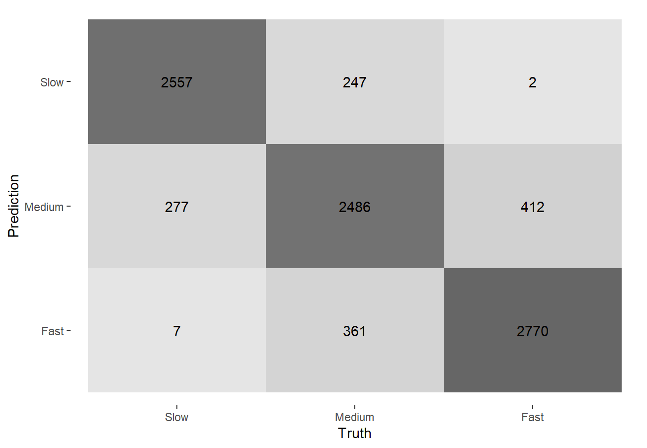

### Interpretation of metrics

Our model achieves excellent performance in predicting delivery speed classes (Slow, Medium, Fast) using only pre-delivery features — with no data leakage — making it operationally trustworthy.

6.6.2.1 ✅ Overall Accuracy & Discrimination

Macro F1 = 0.858: The model balances precision and recall well across all three classes — meaning it doesn’t favor one class at the expense of others.
ROC AUC (Hand & Till) = 0.967: Near-perfect ability to rank deliveries correctly — if we were to sort all orders by predicted “fastness,” the true fastest would almost always appear at the top.

This suggests the model is not just guessing — it’s capturing real patterns in driver behavior, traffic, weather, and geography.

6.6.2.2 🔍 Confusion Matrix Insights

Prediction Truth	Slow	Medium	Fast
Slow	2557	247	2
Medium	277	2486	412
Fast	7	361	2770

6.6.2.2.1 1. “Slow” predictions are highly accurate

2557/2836 = 90% of actual “Slow” deliveries are correctly predicted as “Slow”.
Only 2 misclassified as “Fast” → extremely rare overestimation of speed.
Implication: When the model predicts “Slow”, operations can confidently allocate buffer time or notify customers early.

6.6.2.2.2 2. “Fast” predictions are precise but slightly conservative

2770/2777 = 99.7% of predicted “Fast” deliveries are truly fast → very low false positives.
But 361 “Fast” deliveries were misclassified as “Medium” → some true fast deliveries are being under-predicted.
Implication: We’re not misleading customers with false “Fast” promises — but we might be missing opportunities to highlight truly fast deliveries for marketing or loyalty programs.

6.6.2.2.3 3. “Medium” is the hardest class to predict

2486 correct out of 3165 total → ~78.5% accuracy for this class.
Misclassifications:
- 277 → “Slow” (under-prediction)
- 412 → “Fast” (over-prediction)
Implication: “Medium” is the “gray zone” — perhaps due to borderline cases (e.g., moderate traffic + experienced driver). We should consider adding a “Medium-Fast” or “Medium-Slow” subclass if operational granularity is needed.

6.6.2.3 🧭 Business Recommendations

Here are some recommendations we could draw from this model:

Use Case	Action
Customer ETAs	Use “Fast” predictions to promise tighter windows; use “Slow” to add buffers.
Driver Dispatch	Assign high-rated drivers to “Slow”-predicted orders to improve SLA.
Marketing / Loyalty	Highlight “Fast” deliveries with badges or rewards — model is very reliable here.
Operational Alerts	Flag “Slow” predictions for real-time intervention (reroute, additional help).
Model Refinement	Focus on improving “Medium” prediction — perhaps engineer features like “driver-experience × distance” or “weather-severity index”.

6.6.2.4 🎯 Why This Matters

In food delivery, timing is everything: - Over-promise → customer dissatisfaction. - Under-promise → lost revenue from missed upsells or delayed marketing. - Our model strikes the right balance — accurate, conservative where it matters, and exceptionally discriminative.

The near-perfect ROC AUC (0.967) confirms the model understands relative speed ordering — critical for dynamic pricing, surge alerts, or route optimization.

6.6.2.5 ✅ Final Verdict

This is a production-ready, time-respecting, multiclass classifier that delivers actionable insights without data leakage.
It performs best on extreme classes (Slow and Fast) and decently on the ambiguous middle — exactly what you’d expect from real-world delivery data.

We’ve built a model that’s not just statistically sound, but operationally valuable. 🚀

6.7 🤺 Your turn: experiment with different strategies

Try at least one of the following:

Compare step_upsample() vs step_downsample().
Tune the model again after balancing.
Try a different classifier entirely and note how its sensitivity to imbalance differs.

Summarize your results in a short paragraph.

✅One possible solution

As explained above, downsampling/upsampling can’t be used with time-aware cross-validation: both would break the chronological order of the data and introduce data leakage. We already trialled class weights instead to help with balancing.

References

Lundberg, Scott M, and Su-In Lee. 2017. “A Unified Approach to Interpreting Model Predictions.” In Advances in Neural Information Processing Systems, edited by I. Guyon, U. Von Luxburg, S. Bengio, H. Wallach, R. Fergus, S. Vishwanathan, and R. Garnett. Vol. 30. Curran Associates, Inc. https://proceedings.neurips.cc/paper_files/paper/2017/file/8a20a8621978632d76c43dfd28b67767-Paper.pdf.

1 Introduction

2 🎯 Learning objectives

3 ⚙️ Set-up

3.1 Download dataset and solution notebook

3.2 Install needed libraries

3.3 Import needed libraries

4 🍊 Orange-juice warm-up

4.1 Load and explore the data

4.2 Sampling and stratified splitting

4.3 Feature engineering: add a season variable

4.4 Understanding recipes

4.4.1 Center vs scale vs normalize

4.5 Choose a model

4.6 Build a workflow

4.7 Fit and evaluate the model

4.7.1 How fit() and predict() work

4.7.2 Choosing appropriate metrics

5 Food delivery dataset 🛵

5.1 Load and explore the data

5.2 Create a seasonal feature

5.3 Compute a simple distance feature

5.4 Create time-of-day features

5.4.1 🌆 Why this matters

5.4.2 💡 How these features work together

5.4.3 🕐 Why keep both numeric and categorical forms?

5.5 Create a cross-sectional dataset and training/test split

5.6 Handle missing data with bagged-tree imputation

5.6.1 What is bagged-tree imputation?

5.6.2 🔎 Confirming overlaps among derived time features

5.7 🔍 Key Insights

5.7.1 1. Shared missingness trend across multiple fields

5.7.2 2. Consistent propagation of timestamp missingness

5.7.3 3. multiple_deliveries has lower but correlated missingness

5.7.4 4. No Evidence of MNAR (Missing Not at Random)

5.8 🧠 Interpretation Summary

5.8.1 ✅ Summary Takeaway

5.9 Build a regression recipe

5.9.1 ⚠️ Note on leakage

5.9.2 🧭 1. update_role(...): protect non-predictors and avoid leakage

5.9.3 🧩 2. step_impute_bag(...): principled missing-data handling

5.9.4 🧱 3. step_dummy(all_nominal_predictors()): turn categories into signals

5.9.5 📏 4. step_normalize(all_numeric_predictors()): consistent scales

5.9.6 🧼 5. step_zv(all_predictors()): remove dead columns

5.10 Choose and specify a regression model – LightGBM

5.10.1 Example specification

5.10.2 Common LightGBM tuning parameters

5.11 Combine recipe and model inside a workflow

5.12 Evaluate the cross-sectional model

5.12.1 1️⃣ Accuracy of time predictions

5.12.2 2️⃣ How much variation the model explains

5.12.3 3️⃣ What this means in practice

5.12.4 4️⃣ Important caveat: one week ≠ the whole story

5.12.5 Cross-validation on the cross-sectional data

5.13 Time-aware validation with sliding_period()

5.13.1 How sliding_period() works

5.14 Recipe, workflow, and modeling for longitudinal validation

5.14.1 🧭 Explanation

5.14.1.1 1. Roles updated like the cross-sectional recipe

5.14.1.2 2. Imputation covers all known-missing columns

5.14.1.3 3. step_novel() — essential for unseen levels

5.14.1.4 4. Normalization kept for generality

5.15 Challenge: comparing designs

5.15.1 🔍 Summary of results

5.15.2 🧭 Interpretation

5.16 🧗 Challenge: try another model

5.16.1 💡 Example models (and specification)

5.17 🔁 Elastic Net regression – cross-sectional design

5.18 ⏳ Elastic Net regression – longitudinal (time-aware) design

5.19 Selecting the best models

5.20 🏁 Comparison of finalized models

5.20.1 🚀 Key Takeaways

5.20.2 🔍 Metric-by-Metric Interpretation

5.20.2.1 1. RMSE (Root Mean Squared Error)

5.20.2.2 2. MAE (Mean Absolute Error)

5.20.2.3 3. R² (Coefficient of Determination)

5.20.3 🤔 Why is LightGBM so much better?

5.20.4 💡 Business Implications

5.20.5 ⚠️ Caveat

5.21 🔍 Comparing coefficients and feature importance

5.21.1 Interpretation

4.4 Understanding `recipes`

4.7.1 How `fit()` and `predict()` work

5.7.3 3. `multiple_deliveries` has lower but correlated missingness

5.9.2 🧭 1. `update_role(...)`: protect non-predictors and avoid leakage

5.9.3 🧩 2. `step_impute_bag(...)`: principled missing-data handling

5.9.4 🧱 3. `step_dummy(all_nominal_predictors())`: turn categories into signals

5.9.5 📏 4. `step_normalize(all_numeric_predictors())`: consistent scales

5.9.6 🧼 5. `step_zv(all_predictors())`: remove dead columns

5.13 Time-aware validation with `sliding_period()`

5.13.1 How `sliding_period()` works

5.14.1.3 3. `step_novel()` — essential for unseen levels