Tutorial: `tidymodels` recipes and workflows

From orange juice 🍊 to food delivery 🛵

Author

Published

31 Oct 2025

1 Introduction

Modern data analysis is much more than “fit a model.”
Before a model can learn, we must understand the problem, prepare and clean the data, train, and evaluate it fairly and repeatably.
The tidymodels ecosystem in R provides a unified grammar for all these steps.

In this assignment you will:

explore how recipes describe and execute data-preparation steps,
see how workflows bundle preprocessing and modeling together to prevent data leakage, and
practice building, validating, and comparing models on two datasets.

We begin with a small orange juice dataset 🍊 to introduce tidymodels concepts clearly,
then move on to a larger, more realistic food delivery dataset 🛵.

2 🎯 Learning objectives

By the end of this assignment, you will be able to:

explain what tidymodels recipes and workflows are and why they prevent leakage,
build preprocessing recipes that handle categorical and numeric variables safely,
combine preprocessing and modeling inside workflows,
evaluate models with both random and time-aware cross-validation,
tune and compare model types (e.g. LightGBM, SVM, regularized regression),
engineer meaningful features such as distance and speed, and
address class imbalance through undersampling and oversampling.

3 ⚙️ Set-up

3.1 Download dataset and notebook

You can download the dataset used from section 5 of this tutorial by clicking on the button below:

Just like with all data in this course, place this new dataset into the data folder you created a few weeks ago.

You can also download the notebook that goes with this tutorial by clicking the button below:

3.2 Install needed libraries

install.packages('ISLR2')
install.packages('geosphere')
install.packages('lightgbm')
install.packages('bonsai')
install.packages('vip')

or if you have the librarian library installed:

librarian::shelf(ISLR2,geosphere,lightgbm,bonsai,vip)

3.3 Import needed libraries

library(tidymodels)
library(ISLR2)
library(tidyverse)
library(lubridate)
library(geosphere)
library(bonsai)
library(ggplot2)

LightGBM and the bonsai package

The tidymodels core packages (like parsnip) define the modeling interface but not every possible engine.
Support for LightGBM is provided by an extension package called bonsai, which connects tree-based algorithms like LightGBM and CatBoost to the tidymodels syntax.

4 🍊 Orange-juice warm-up

The aim of this section is to understand the logic of tidymodels through a compact, complete example.
You will predict which brand of orange juice a customer buys—Citrus Hill (CH) or Minute Maid (MM)—using price, discounts, and loyalty information.

4.1 Load and explore the data

data(OJ)
glimpse(OJ)

Rows: 1,070
Columns: 18
$ Purchase       <fct> CH, CH, CH, MM, CH, CH, CH, CH, CH, CH, CH, CH, CH, CH,…
$ WeekofPurchase <dbl> 237, 239, 245, 227, 228, 230, 232, 234, 235, 238, 240, …
$ StoreID        <dbl> 1, 1, 1, 1, 7, 7, 7, 7, 7, 7, 7, 7, 7, 7, 7, 7, 1, 2, 2…
$ PriceCH        <dbl> 1.75, 1.75, 1.86, 1.69, 1.69, 1.69, 1.69, 1.75, 1.75, 1…
$ PriceMM        <dbl> 1.99, 1.99, 2.09, 1.69, 1.69, 1.99, 1.99, 1.99, 1.99, 1…
$ DiscCH         <dbl> 0.00, 0.00, 0.17, 0.00, 0.00, 0.00, 0.00, 0.00, 0.00, 0…
$ DiscMM         <dbl> 0.00, 0.30, 0.00, 0.00, 0.00, 0.00, 0.40, 0.40, 0.40, 0…
$ SpecialCH      <dbl> 0, 0, 0, 0, 0, 0, 1, 1, 0, 0, 0, 0, 0, 0, 0, 0, 0, 0, 0…
$ SpecialMM      <dbl> 0, 1, 0, 0, 0, 1, 1, 0, 0, 0, 0, 0, 1, 0, 0, 0, 1, 1, 0…
$ LoyalCH        <dbl> 0.500000, 0.600000, 0.680000, 0.400000, 0.956535, 0.965…
$ SalePriceMM    <dbl> 1.99, 1.69, 2.09, 1.69, 1.69, 1.99, 1.59, 1.59, 1.59, 1…
$ SalePriceCH    <dbl> 1.75, 1.75, 1.69, 1.69, 1.69, 1.69, 1.69, 1.75, 1.75, 1…
$ PriceDiff      <dbl> 0.24, -0.06, 0.40, 0.00, 0.00, 0.30, -0.10, -0.16, -0.1…
$ Store7         <fct> No, No, No, No, Yes, Yes, Yes, Yes, Yes, Yes, Yes, Yes,…
$ PctDiscMM      <dbl> 0.000000, 0.150754, 0.000000, 0.000000, 0.000000, 0.000…
$ PctDiscCH      <dbl> 0.000000, 0.000000, 0.091398, 0.000000, 0.000000, 0.000…
$ ListPriceDiff  <dbl> 0.24, 0.24, 0.23, 0.00, 0.00, 0.30, 0.30, 0.24, 0.24, 0…
$ STORE          <dbl> 1, 1, 1, 1, 0, 0, 0, 0, 0, 0, 0, 0, 0, 0, 0, 0, 1, 2, 2…

Each row describes sales of orange juice for one week in one store. The outcome variable is Purchase, which records whether the customer bought CH or MM.

Other important variables include:

Variable	Description
`PriceCH`, `PriceMM`	prices of Citrus Hill and Minute Maid
`DiscCH`, `DiscMM`	discounts for each brand
`LoyalCH`	loyalty toward Citrus Hill
`STORE`, `WeekofPurchase`	store ID and week number

4.2 Sampling and stratified splitting

The full dataset has just over a thousand rows. To simulate a smaller study, we take a sample of 250 rows and then split it into training and test sets (60 % / 40 %). Because Purchase is categorical, we stratify so the CH/MM ratio remains constant.

Why 60/40 instead of 80/20? When the dataset is small, an 80/20 split leaves very few test examples, making metrics unstable. A 60/40 split provides enough data to train while still leaving a meaningful number of unseen samples for evaluation.

set.seed(123)

oj_sample_split <- initial_split(OJ, prop = 250 / nrow(OJ), strata = Purchase)
oj_sample <- training(oj_sample_split)

oj_split <- initial_split(oj_sample, prop = 0.6, strata = Purchase)
oj_train <- training(oj_split)
oj_test  <- testing(oj_split)

bind_rows(
  OJ        |> count(Purchase) |> mutate(prop = n/sum(n), set = "Full"),
  oj_sample |> count(Purchase) |> mutate(prop = n/sum(n), set = "Sample 250"),
  oj_train  |> count(Purchase) |> mutate(prop = n/sum(n), set = "Train 60%"),
  oj_test   |> count(Purchase) |> mutate(prop = n/sum(n), set = "Test 40%")
)

  Purchase   n      prop        set
1       CH 653 0.6102804       Full
2       MM 417 0.3897196       Full
3       CH 152 0.6104418 Sample 250
4       MM  97 0.3895582 Sample 250
5       CH  91 0.6107383  Train 60%
6       MM  58 0.3892617  Train 60%
7       CH  61 0.6100000   Test 40%
8       MM  39 0.3900000   Test 40%

Why stratify?

Stratification ensures that both training and testing subsets keep the same mix of CH and MM. Without it, we could train mostly on one brand and evaluate on another—a subtle form of bias. Think of the dataset as a smoothie: 60 % orange 🍊 and 40 % mango 🥭. Every smaller glass should taste the same.

4.3 Feature engineering: add a season variable

WeekofPurchase records when the purchase occurred. Week numbers by themselves are not very informative, but they can reveal seasonal patterns—for instance, one brand might sell better in summer.

We’ll create a new column season based on week number and keep WeekofPurchase as a non-predictor identifier.

oj_train <- oj_train |>
  mutate(
    season = case_when(
      WeekofPurchase %% 52 < 13 ~ "Winter",
      WeekofPurchase %% 52 < 26 ~ "Spring",
      WeekofPurchase %% 52 < 39 ~ "Summer",
      TRUE ~ "Fall"
    )
  )

oj_test <- oj_test |>
  mutate(
    season = case_when(
      WeekofPurchase %% 52 < 13 ~ "Winter",
      WeekofPurchase %% 52 < 26 ~ "Spring",
      WeekofPurchase %% 52 < 39 ~ "Summer",
      TRUE ~ "Fall"
    )
  )

4.4 Understanding `recipes`

A recipe is a plan describing exactly how data should be prepared before modeling. It bundles all preprocessing steps so they can be applied identically across training, testing, and resampling.

Here is a complete recipe for our orange-juice problem:

oj_rec <- recipe(Purchase ~ PriceCH + PriceMM + DiscCH + DiscMM +
                   LoyalCH + STORE + season + WeekofPurchase,
                 data = oj_train) |>
  update_role(WeekofPurchase, new_role = "ID") |>  # keep but do not model
  step_dummy(all_nominal_predictors()) |>           # encode categoricals
  step_center(all_numeric_predictors()) |>          # subtract mean
  step_scale(all_numeric_predictors())              # divide by SD

4.4.1 Center vs scale vs normalize

step_center() subtracts each variable’s mean so values are centered at 0.
step_scale() divides by standard deviation so units are comparable.
step_normalize() combines both operations in a single step.

Why standardize? Models such as logistic regression, SVMs, and KNN are sensitive to variable scales. Standardizing puts all numeric predictors on a common footing and stabilizes optimization.

4.5 Choose a model

We will use logistic regression for this classification task.

oj_mod <- logistic_reg() |> set_engine("glm")

4.6 Build a workflow

A workflow combines preprocessing and modeling so that the correct steps are always applied in the correct order.

oj_wf <- workflow() |>
  add_recipe(oj_rec) |>
  add_model(oj_mod)

4.7 Fit and evaluate the model

oj_fit <- oj_wf |> fit(data = oj_train)

oj_probs <- predict(oj_fit, oj_test, type = "prob")
oj_class <- predict(oj_fit, oj_test)

oj_preds <- bind_cols(oj_test |> select(Purchase), oj_probs, oj_class)

# class-based metrics
class_metrics <- metric_set(f_meas, precision, recall)

class_metrics(oj_preds,
              truth = Purchase,
              estimate = .pred_class)

# probability-based metric
roc_auc(oj_preds, truth = Purchase, .pred_CH)

# A tibble: 3 × 3
  .metric   .estimator .estimate
  <chr>     <chr>          <dbl>
1 f_meas    binary         0.887
2 precision binary         0.873
3 recall    binary         0.902

roc_auc(oj_preds, truth = Purchase, .pred_CH)
# A tibble: 1 × 3
  .metric .estimator .estimate
  <chr>   <chr>          <dbl>
1 roc_auc binary         0.923

4.7.1 How `fit()` and `predict()` work

When you call fit(), tidymodels first trains the recipe on the training data: it computes the statistics required for preprocessing—means and standard deviations for scaling, the set of levels for categorical variables, etc.—and stores them inside the workflow. It then fits the model (here, a logistic regression) to the processed training data.

Later, predict() re-applies the trained recipe to the test data using those same stored statistics. No new averages or encodings are computed; the test data remain unseen during training. This is what prevents data leakage—the model never peeks at future information.

4.7.2 Choosing appropriate metrics

Because the classes are not perfectly balanced, accuracy can be misleading. A model that always predicts the majority class might look “accurate” but tell us little. Instead we evaluate:

Precision: when the model predicts CH, how often is it correct?
Recall: of all actual CH purchases, how many did it find?
F₁-score: the harmonic mean of precision and recall, balancing both.
ROC AUC: the area under the ROC curve, summarizing discrimination across thresholds.

These measures together give a more complete picture of performance.

Your turn🤺

Replace logistic_reg() with another classifier you know, such as rand_forest() or svm_rbf().
Rerun the recipe, workflow, and evaluation.
Compare F₁ and ROC AUC. Which model performs better, and why might that be?

5 Food delivery dataset 🛵

You are now ready to apply the same ideas to a realistic dataset.
We will use a public Food Delivery dataset from Kaggle containing restaurant, delivery-person, and environmental details along with the delivery time in minutes (we’re using the dataset called train on Kaggle).

Your objectives are to:

Predict delivery time (Time_taken(min)) using regression.
Compare cross-sectional and time-aware validation.
Later, classify deliveries by speed.

5.1 Load and explore the data

food <- read_csv("data/food-delivery.csv") |>
  mutate(
    Order_Date = dmy(Order_Date),
    Order_Week = isoweek(Order_Date)
  ) |>
  arrange(Order_Date)

glimpse(food)

Rows: 45,593
Columns: 21
$ ID                          <chr> "0xd936", "0xd681", "0xc606", …
$ Delivery_person_ID          <chr> "GOARES15DEL02", "GOARES07DEL0…
$ Delivery_person_Age         <dbl> 26, 38, 20, 39, 20, 33, 21, 29…
$ Delivery_person_Ratings     <dbl> 4.3, 4.9, 4.5, 4.7, 4.8, 4.6, …
$ Restaurant_latitude         <dbl> 15.51315, 15.56129, 0.00000, 2…
$ Restaurant_longitude        <dbl> 73.78346, 73.74948, 0.00000, 8…
$ Delivery_location_latitude  <dbl> 15.56315, 15.60130, 0.05000, 2…
$ Delivery_location_longitude <dbl> 73.83346, 73.78948, 0.05000, 8…
$ Order_Date                  <date> 2022-02-11, 2022-02-11, 2022-…
$ Time_Orderd                 <chr> "23:25:00", "13:35:00", "21:10…
$ Time_Order_picked           <time> 23:35:00, 13:40:00, 21:25:00,…
$ Weatherconditions           <chr> "conditions Sandstorms", "cond…
$ Road_traffic_density        <chr> "Low", "High", "Jam", "Low", "…
$ Vehicle_condition           <dbl> 0, 1, 1, 1, 2, 1, 1, 2, 2, 1, …
$ Type_of_order               <chr> "Buffet", "Drinks", "Drinks", …
$ Type_of_vehicle             <chr> "motorcycle", "scooter", "moto…
$ multiple_deliveries         <dbl> 0, 1, 1, 0, 1, 1, 1, 1, 1, 1, …
$ Festival                    <chr> "No", "No", "No", "No", "No", …
$ City                        <chr> "Urban", "Urban", "Metropoliti…
$ `Time_taken(min)`           <chr> "(min) 21", "(min) 25", "(min)…
$ Order_Week                  <dbl> 6, 6, 6, 6, 6, 6, 6, 6, 6, 6, …

The dataset includes restaurant and delivery coordinates, information about the delivery person, weather, traffic, and more. We first convert Order_Date from a string into a proper Date object using dmy() so R recognizes it as a date. Then we create Order_Week (the ISO week number) to group all orders from the same week.

Why group by week rather than day or month? Daily data can be too granular—many days may have only a few deliveries—whereas monthly data hide short-term fluctuations. Grouping by week is a reasonable middle ground for time-aware validation later.

🤺 Your turn: clean up the delivery time variable

The variable Time_taken(min) is stored as text values such as "(min) 21". Convert it to numeric values like 21 using a suitable string operation and transformation.

💡 Question: Why do you think this conversion is important before modeling?

5.2 Create a seasonal feature

While Order_Week captures time numerically, sometimes it’s more interpretable to group weeks into seasons. Since all orders here fall between February and April, we can label them roughly as “late winter” or “early spring.”

food <- food |>
  mutate(
    Season = case_when(
      Order_Week %in% 1:13   ~ "Winter",   # Weeks 1–13 (approx. Jan–Mar)
      Order_Week %in% 14:26  ~ "Spring",   # Weeks 14–26 (Apr–Jun)
      Order_Week %in% 27:39  ~ "Summer",   # Weeks 27–39 (Jul–Sep)
      Order_Week %in% 40:52  ~ "Autumn",   # Weeks 40–52 (Oct–Dec)
      TRUE ~ NA_character_
    )
  )

You can then decide whether to:

Use Season as a categorical predictor (it will be converted into dummy variables by your recipe), or
Treat it as a non-predictor context variable using update_role(Season, new_role = "ID").

Both approaches are valid, depending on your modeling goal.

🌱 Why this matters

Creating seasonal or cyclical indicators helps the model capture periodic effects (for instance, delivery conditions in early spring vs. late winter) without memorizing specific weeks.

5.3 Compute a simple distance feature

Delivery time should depend strongly on distance. We can approximate distance using the Haversine formula, which computes the great-circle (shortest) distance between two points on Earth.

food <- food |>
  mutate(distance_km = distHaversine(
    cbind(Restaurant_longitude, Restaurant_latitude),
    cbind(Delivery_location_longitude, Delivery_location_latitude)
  ) / 1000)

Why distance matters

Even a rough, straight-line distance captures a large share of the variation in delivery times. It reflects the physical effort of travel even when we do not model exact routes or traffic lights.

Why this is safe before splitting

Each distance_km value depends only on its own row (restaurant and delivery coordinates). No information is averaged or shared across the dataset, so calculating this feature before splitting does not cause leakage.

5.4 Create time-of-day features

Delivery times don’t depend solely on distance or traffic — they also vary throughout the day. Morning commutes, lunch peaks, and late-night orders each impose different operational pressures on both restaurants and delivery drivers.

We’ll capture these daily patterns by creating new variables describing the time of order placement and time of pickup, both as numeric hours and as interpretable day-part categories.

food <- food |>
  mutate(
    # Clean invalid or empty time strings
    Time_Orderd = na_if(Time_Orderd, "NaN"),
    Time_Orderd = na_if(Time_Orderd, ""),
    Time_Orderd = na_if(Time_Orderd, "null"),
    Time_Orderd = na_if(Time_Orderd, "0"),

    # Then safely extract hours, using suppressWarnings() to ignore harmless NAs
    Order_Hour = suppressWarnings(lubridate::hour(hms::as_hms(Time_Orderd))),
    Pickup_Hour = suppressWarnings(lubridate::hour(hms::as_hms(Time_Order_picked))),

    # Categorical time-of-day bins (use the numeric hours we just extracted)
    Time_of_Day = case_when(
      Pickup_Hour >= 5  & Pickup_Hour < 12 ~ "Morning",
      Pickup_Hour >= 12 & Pickup_Hour < 17 ~ "Afternoon",
      Pickup_Hour >= 17 & Pickup_Hour < 22 ~ "Evening",
      TRUE                                 ~ "Night"
    ),
    Order_Time_of_Day = case_when(
      is.na(Order_Hour)                  ~ NA_character_,
      Order_Hour >= 5  & Order_Hour < 12 ~ "Morning",
      Order_Hour >= 12 & Order_Hour < 17 ~ "Afternoon",
      Order_Hour >= 17 & Order_Hour < 22 ~ "Evening",
      TRUE                               ~ "Night"
    )

  )

Warning

⚠️ Some entries in Time_Orderd are invalid (e.g., "NaN", "", or "0") and can’t be converted to clock times. To avoid errors, we explicitly set these to NA before parsing. Missing times are later handled by the recipe’s step_impute_bag(), which fills them using information from other predictors.

⚠️ Handling missingness correctly in derived features

When deriving categorical summaries from numeric variables (like converting Order_Hour to Order_Time_of_Day), you must explicitly preserve missingness.

By default, case_when() assigns the “else” case (TRUE ~ ...) even when inputs are missing. This can make downstream missingness disappear artificially, hiding real data problems.

If Order_Hour is missing because the original Time_Orderd was invalid or blank, we should preserve that NA in the derived column — otherwise, the model might think those rows are “Night” orders!

5.4.1 🌆 Why this matters

Raw timestamps like "13:42:00" are hard for models to interpret: they’re too granular, cyclical (23:59 ≈ 00:01), and numerically meaningless. By extracting hour values and day-part categories, we make time information explicit and interpretable.

Feature	Type	Operational meaning	Expected effect on delivery time
`Order_Hour`	Numeric (0–23)	The exact hour when the customer placed the order	Reflects demand cycles — lunch (12–14h) and dinner (19–21h) peaks increase restaurant load and prep time.
`Pickup_Hour`	Numeric (0–23)	The exact hour when the courier picked up the order	Reflects road and traffic conditions — peak commute hours (8–10h, 17–20h) slow travel.
`Order_Time_of_Day`	Categorical (Morning/Afternoon/Evening/Night)	Coarse summary of restaurant-side demand	Morning orders (e.g., breakfast deliveries) tend to be faster; dinner rushes slower.
`Time_of_Day`	Categorical (Morning/Afternoon/Evening/Night)	Coarse summary of driver-side conditions	Evening and night deliveries face heavier congestion and longer travel times.

5.4.2 💡 How these features work together

The order and pickup stages represent two distinct time-sensitive parts of the end-to-end delivery process:

Stage	Key processes	Feature(s)	What it captures
1. Order placement → pickup	Kitchen preparation, queueing, and coordination delays	`Order_Hour`, `Order_Time_of_Day`	Busy restaurant periods (e.g., lunch) slow down order readiness.
2. Pickup → delivery completion	Driving, navigation, and drop-off conditions	`Pickup_Hour`, `Time_of_Day`	Traffic congestion, daylight, and road conditions affect delivery speed.

Together, these features let the model separate restaurant-side delays from driver-side delays — two sources that are often conflated in the overall Time_taken(min) target.

🧩 For example:

Orders placed at 12:00 but picked up at 12:40 suggest restaurant bottlenecks.

Deliveries picked up at 18:00 tend to face evening rush-hour slowdowns, even for the same distance.

This dual-stage representation helps the model uncover more realistic, interpretable patterns in how delivery times fluctuate across the day.

5.4.3 🕐 Why keep both numeric and categorical forms?

Representation	Strength	When it helps
Numeric (`Order_Hour`, `Pickup_Hour`)	Retains the continuous structure of time (e.g., 10 → 11 → 12), enabling models to learn smooth nonlinear effects.	Particularly useful for tree-based models (like LightGBM) that can detect thresholds or local increases.
Categorical (`Order_Time_of_Day`, `Time_of_Day`)	Encodes interpretable shifts between broad periods (morning vs evening) and captures discontinuous behavior (e.g., lunch/dinner rushes).	Helpful for communicating and visualizing time effects and for linear models needing explicit contrasts.

Tree-based models can seamlessly decide which variant carries the stronger signal for prediction.

5.5 Create a cross-sectional dataset and training/test split

A cross-sectional analysis takes one time period and treats all observations within it as independent. We will use the busiest week (the one with the most orders).

week_counts <- food |> count(Order_Week, sort = TRUE)

cross_df <- food |>
  filter(Order_Week == first(week_counts$Order_Week))

Why the busiest week? It provides enough examples for both training and validation within a consistent operational context (similar traffic, weather, and demand). Smaller weeks may have too few deliveries to form stable training and test sets, and combining non-adjacent weeks might mix different traffic or weather patterns. This design isolates one dense period to study model behavior without temporal drift.

🤺 Your turn: create the split

Split the cross_df data into training and test sets. Use about 80 % of the data for training and 20 % for testing. Set a random seed for reproducibility.

5.6 Handle missing data with bagged-tree imputation

Only a few predictors contain missing data:

Delivery_person_Ratings
Delivery_person_Age
multiple_deliveries

Rather than filling these with simple averages or modes, we will impute them using bagged-tree models.

5.6.1 What is bagged-tree imputation?

Bagging stands for bootstrap aggregation. It works as follows:

Draw multiple bootstrap samples from the available (non-missing) data. Each bootstrap sample is drawn with replacement, meaning some observations appear more than once while others are left out.
Fit a small decision tree to each bootstrap sample to predict the missing variable from all others.
For each missing entry, average the predictions across all trees.

Because each tree sees a slightly different subset, their averaged predictions are more stable and less biased than any single model.

This process is closely related to Random Forests, which also reduce variance by averaging many decorrelated trees. The main difference is that Random Forests use random subsets of predictors as well as bootstrap samples, while bagging only resamples the data.

Bagged-tree imputation therefore preserves relationships among variables while smoothing out noise and avoiding the distortions that mean or mode imputation can cause.

🤺 Your turn: check missingness

Before you decide how to impute, always explore where data are missing.

Use functions such as summary(), skimr::skim(), or naniar::miss_var_summary() to inspect missing values in each column.
Identify which variables have the most missingness.
Write two or three sentences: do you think the missingness is random or related to certain conditions (e.g., specific cities, traffic levels, or festivals)?

5.7 Build a regression recipe

You will now create a recipe that predicts Time_taken(min) from reasonable predictors. Do not copy a pre-written recipe here — write your own using the tidymodels recipes reference: https://recipes.tidymodels.org/reference/index.html

Your recipe should:

Impute missing values with bagged trees (step_impute_bag()).
Convert categorical predictors to dummy variables (step_dummy()).
Normalize all numeric predictors (step_normalize()).
Remove zero-variance predictors (step_zv()).

5.7.1 ⚠️ Note on leakage

Always create and train your recipe after splitting the data. Defining the recipe is fine on the full dataset — it’s just a blueprint — but prep() must only ever be applied to the training data. tidymodels enforces this automatically when you put the recipe inside a workflow().

5.8 Choose and specify a regression model – LightGBM

We will use LightGBM, a modern gradient-boosted-tree algorithm that is very efficient on large tabular data.

Both LightGBM and XGBoost implement gradient boosting: a sequence of small trees is trained, each correcting residual errors from previous trees. The difference lies in how they grow trees and manage splits:

XGBoost grows trees level-wise (balanced): it splits all leaves at one depth before going deeper. This produces symmetric trees and is often robust on small or moderately sized data.
LightGBM grows trees leaf-wise: it always expands the single leaf that most reduces the loss, yielding deeper, targeted trees. Together with histogram-based binning of features, this makes LightGBM faster and often stronger on large, sparse, or high-cardinality data.

5.8.1 Example specification

lgb_mod <- boost_tree(
  trees = 500,
  learn_rate = 0.1,
  tree_depth = 6,
  loss_reduction = 0.0,
  min_n = 2
) |>
  set_engine("lightgbm") |>
  set_mode("regression")

5.8.2 Common LightGBM tuning parameters

Parameter	What it controls	Intuition
`trees`	total number of trees	more trees can capture more structure but risk overfitting unless `learn_rate` is small
`learn_rate`	step size for each tree’s contribution	small = slower but safer learning; large = faster but riskier
`tree_depth`	maximum depth of a single tree	deeper trees capture complex interactions but can overfit
`loss_reduction`	minimum loss reduction to make a split	larger values prune weak splits and simplify trees
`min_n`	minimum observations in a leaf	prevents tiny leaves that memorize noise
`mtry`	number of predictors sampled at each split	adds randomness, reduces correlation among trees

When might you prefer XGBoost? On smaller datasets, when stability and interpretability matter. When might you prefer LightGBM? For speed on larger tables, many categorical dummies, or limited tuning time.

5.9 Combine recipe and model inside a workflow

Once your recipe and model specification are ready, combine them with workflow() so preprocessing and modeling stay linked. Workflows automatically apply the recipe before fitting or predicting.

# your workflow code here

5.10 Evaluate the cross-sectional model

Fit your workflow on the training set and evaluate predictions on the test set.
Use regression metrics such as RMSE, MAE, and R².

🤺 Your turn

Compute and report these metrics for your model.
How accurate is the model on unseen data?
Does it tend to over- or under-predict delivery time?

5.10.1 Cross-validation on the cross-sectional data

So far, you evaluated the model with a single train/test split. In a cross-sectional setting (no time ordering), it is common to use k-fold cross-validation, which splits the training data into k random folds, training on k – 1 folds and validating on the remaining fold in turn. This yields a more robust estimate of performance stability.

set.seed(42)
cv_cross <- vfold_cv(cross_train, v = 5)

cross_cv_res <- fit_resamples(
  reg_wf,
  resamples = cv_cross,
  metrics = metric_set(rmse, mae, rsq),
  control = control_resamples(save_pred = TRUE)
)

collect_metrics(cross_cv_res)

🤺 Your turn

Run a 5-fold cross-validation on the cross-sectional training data. Compare the average RMSE and R² to those from the single test-set evaluation. Are they similar? Which estimate do you trust more?

5.11 Time-aware validation with `sliding_period()`

In time-dependent data, future information must not influence the model’s training. To mimic real-world deployment, we roll forward through time: train on past weeks, validate on the next week(s).

# create a chronological split first
set.seed(42)
long_split <- initial_time_split(food, prop = 0.8)
long_train <- training(long_split)
long_test  <- testing(long_split)

cv_long <- sliding_period(
  data        = long_train,  # your longitudinal training data (not the full dataset!)
  index       = Order_Date,
  period      = "week",
  lookback    = Inf,        # how many past weeks form the training window
  assess_stop = 1         # how many future weeks form the validation window
)

⚠️ Avoid leakage!

Never define cross-validation folds on the entire dataset. If you did, the model could “peek” at future data while training, inflating performance. Instead, use only the training portion of your longitudinal split—here called long_train.

5.11.1 How `sliding_period()` works

sliding_period() creates a sequence of rolling resamples ordered by the variable given in index. Here, the index is Order_Date, which is of class Date. Because it understands the class of this variable, rsample can interpret the keyword period = "week" as:

“Use the calendar weeks implied by the Date variable to move the window forward one week at a time.”

Internally, it uses date arithmetic (floor_date() and ceiling_date() logic) to determine where each new week starts and stops. If you had specified period = "day" or period = "month", it would instead roll forward daily or monthly. Thus, period defines the temporal granularity of each split, and index provides the timeline to follow.

Peering inside the cross-validation folds

Let’s try and have a look at which dates the sliding_period() cross-validation folds correspond to:

cv_long_summary <- cv_long %>%
  mutate(
    train_start = map(splits, ~ min(analysis(.x)$Order_Date)),
    train_end   = map(splits, ~ max(analysis(.x)$Order_Date)),
    val_start   = map(splits, ~ min(assessment(.x)$Order_Date)),
    val_end     = map(splits, ~ max(assessment(.x)$Order_Date))
  ) %>%
  tidyr::unnest(c(train_start, train_end, val_start, val_end)) %>%
  select(id, train_start, train_end, val_start, val_end)

cv_long_summary

# A tibble: 6 × 5
  id     train_start train_end  val_start  val_end   
  <chr>  <date>      <date>     <date>     <date>    
1 Slice1 2022-02-11  2022-02-16 2022-02-17 2022-02-18
2 Slice2 2022-02-11  2022-02-18 2022-03-01 2022-03-02
3 Slice3 2022-02-11  2022-03-02 2022-03-03 2022-03-09
4 Slice4 2022-02-11  2022-03-09 2022-03-10 2022-03-16
5 Slice5 2022-02-11  2022-03-16 2022-03-17 2022-03-23
6 Slice6 2022-02-11  2022-03-23 2022-03-24 2022-03-29

If you want to have a look at which weeks these folds correspond to instead:

cv_long_summary_weeks <- cv_long %>%
  mutate(
    train_start_wk = map_int(splits, ~ isoweek(min(analysis(.x)$Order_Date))),
    train_end_wk   = map_int(splits, ~ isoweek(max(analysis(.x)$Order_Date))),
    val_start_wk   = map_int(splits, ~ isoweek(min(assessment(.x)$Order_Date))),
    val_end_wk     = map_int(splits, ~ isoweek(max(assessment(.x)$Order_Date)))
  ) %>%
  select(id, train_start_wk, train_end_wk, val_start_wk, val_end_wk)

cv_long_summary_weeks

# A tibble: 6 × 5
  id     train_start_wk train_end_wk val_start_wk val_end_wk
  <chr>           <int>        <int>        <int>      <int>
1 Slice1              6            7            7          7
2 Slice2              6            7            9          9
3 Slice3              6            9            9         10
4 Slice4              6           10           10         11
5 Slice5              6           11           11         12
6 Slice6              6           12           12         13

And if you want to visualise the folds:

cv_long_summary %>%
  mutate(id = factor(id, levels = rev(id))) %>%  # reverse for readability
  ggplot() +
  geom_segment(aes(x = train_start, xend = train_end, y = id, yend = id),
               color = "#0072B2", linewidth = 3) +
  geom_segment(aes(x = val_start, xend = val_end, y = id, yend = id),
               color = "#E69F00", linewidth = 3) +
  labs(
    title = "Expanding Weekly Sliding-Period Cross-Validation",
    x = "Date", y = "Slice",
    caption = "Blue = training window, Orange = validation window"
  ) +
  theme_minimal(base_size = 13)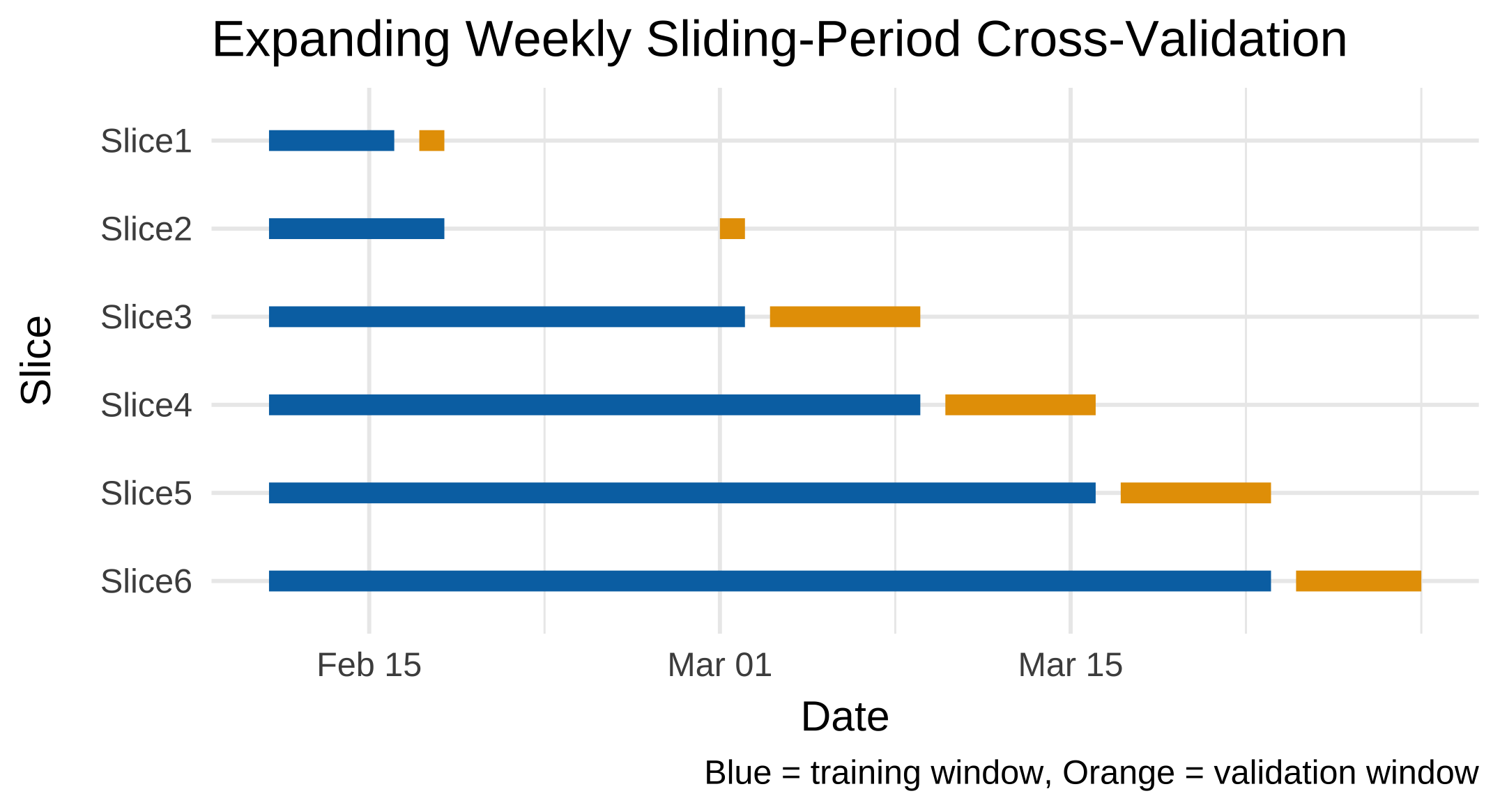

5.12 Recipe, workflow, and modeling for longitudinal validation

Repeat the full process—recipe, model, and workflow—on the longitudinal setup. Then train and evaluate the model using the time-aware resamples created above.

🤺 Your turn

Use fit_resamples() to fit your LightGBM workflow with cv_long. Collect metrics (rmse, mae, rsq) and summarize them.

5.13 Challenge: comparing designs

Compare your cross-sectional and longitudinal results.

💬 Think about this

Are the results directly comparable? Why or why not?
Which design better represents real-world performance, and why?
How does time-aware validation change your interpretation of model quality?

5.14 🧗 Challenge: try another model

Repeat the workflow using a different algorithm of your choice (for example, Elastic-Net, SVM, or KNN). Do not copy specifications here — consult lectures, 📚labs W02–W05, and the reading week homework for syntax, recommended preprocessing, and tuning guidance.

Evaluate the alternative model on both cross-sectional and time-aware folds and compare results.

💭 Reflection

Which model generalized best over time?
Did any model overfit when using random folds but degrade under time-aware validation?
Which preprocessing steps (such as normalization) were essential for your chosen model, and why?
Would your preferred model still perform well if new conditions appeared (e.g., “Summer” deliveries or new cities)?

6 Classifying deliveries by speed 🚴‍♀️

So far, you have treated delivery time as a continuous variable and built regression models to predict it.
We will now reframe the same problem as a classification task: predicting whether a delivery is fast, medium, or slow based on its characteristics.

This shift lets you practice classification workflows and also experiment with techniques for handling class imbalance.

6.1 Define delivery-speed classes

Rather than using arbitrary thresholds (for example “below 30 minutes = fast”),
we can define speed relative to distance.
A fairer comparison is delivery speed = distance / time in km per minute (or per hour).

food <- food |>
  mutate(speed_km_min = distance_km / (`Time_taken(min)`),
         speed_class = case_when(
           speed_km_min >= quantile(speed_km_min, 0.67, na.rm = TRUE) ~ "Fast",
           speed_km_min <= quantile(speed_km_min, 0.33, na.rm = TRUE) ~ "Slow",
           TRUE ~ "Medium"
         )) |>
  mutate(speed_class = factor(speed_class,
                              levels = c("Slow", "Medium", "Fast")))

This approach adapts automatically to the dataset’s scale and ensures that roughly one-third of deliveries fall in each class. You can adjust the quantile cut-offs if you wish to make the “Fast” or “Slow” categories narrower.

Alternative definitions

If you prefer a binary classification (for example fast vs not fast), combine “Slow” and “Medium” into a single category. Think about which framing would be more relevant for an operations team.

6.2 Explore class balance

Always check how balanced your outcome variable is before training models.

food |> count(speed_class) |> mutate(prop = n / sum(n))

# A tibble: 3 × 3
  speed_class     n  prop
  <fct>       <int> <dbl>
1 Slow        15046 0.330
2 Medium      15501 0.340
3 Fast        15046 0.330

In this case, the classes are roughly balanced (though Medium has a few more samples).

6.3 🤺 Your turn: build a classification recipe

Split the data into training/test sets and create a recipe that predicts speed_class from the relevant predictors (distance, traffic, weather, vehicle type, etc.).

Follow the same logic as before but adapt it for classification:

Impute missing values with bagged trees (step_impute_bag()).
Convert categorical variables to dummies (step_dummy()).
Normalize numeric predictors (step_normalize()).
Optionally include a resampling step such as step_upsample() or step_downsample() to address class imbalance.

Consult the recipes documentation (https://recipes.tidymodels.org/reference/index.html) for details.

Tip

You can include resampling steps directly inside a recipe so they are applied each time data are resampled during training. For instance:

step_upsample(speed_class)

will randomly duplicate minority-class examples inside each resample, while step_downsample(speed_class) will randomly discard some majority-class examples.

⚠️ Important:

Upsampling and downsampling assume that observations can be freely shuffled between resamples. They are suitable for random cross-validation, where all rows are exchangeable. However, they should not be used inside time-aware cross-validation such as sliding_period(). Doing so would destroy the chronological structure and introduce future information into past folds, leading to data leakage. If you wish to handle imbalance in time-series data, use class-weighting or design metrics that account for imbalance instead.

6.4 Choose a classification model

Select any classifier you are comfortable with—examples include:

Logistic regression (baseline, interpretable)
Support-Vector Machine (SVM)
K-Nearest Neighbors (KNN)
Balanced Random Forest (handles imbalance well)
LightGBM (fast and strong gradient boosting)

Use your lecture notes and 📚 labs W02–W05 for parameter syntax and typical preprocessing needs.

Combine your model with the recipe in a workflow as before:

class_wf <- workflow() |>
  add_recipe(your_class_recipe) |>
  add_model(your_model_spec)

6.5 Resampling and cross-validation

Decide whether to evaluate your classification model on:

the cross-sectional subset (the busiest week), or
the time-aware folds (cv_long).

You may reuse the resample objects created earlier. Perform tuning where appropriate (for example, the number of neighbors in KNN or cost in SVM). Refer again to the 📚W05 lab for tuning model hyperparameters with tune_grid().

6.6 Evaluate classification performance

For classification problems, accuracy alone can be misleading under imbalance. Instead, report metrics such as:

Metric	Meaning
Precision	How often predicted “Fast” deliveries were truly fast
Recall	How many actual fast deliveries were found
F₁-score	Balance of precision and recall
ROC AUC	Discrimination across thresholds
PR AUC	Area under the precision-recall curve (useful when positives are rare)

metric_set(precision, recall, f_meas, roc_auc, pr_auc)(
  predictions,
  truth = speed_class,
  estimate = .pred_class
)

If you used step_upsample() or step_downsample(), compare performance with and without the balancing step.

Questions

Did balancing improve recall for the minority class?
Which metric changed most after balancing?
Would you recommend oversampling or undersampling for this dataset, and why?

6.7 🤺 Your turn: experiment with different strategies

Try at least one of the following:

Compare step_upsample() vs step_downsample().
Tune the model again after balancing.
Try a different classifier entirely and note how its sensitivity to imbalance differs.

Summarize your results in a short paragraph.

1 Introduction

2 🎯 Learning objectives

3 ⚙️ Set-up

3.1 Download dataset and notebook

3.2 Install needed libraries

3.3 Import needed libraries

4 🍊 Orange-juice warm-up

4.1 Load and explore the data

4.2 Sampling and stratified splitting

4.3 Feature engineering: add a season variable

4.4 Understanding recipes

4.4.1 Center vs scale vs normalize

4.5 Choose a model

4.6 Build a workflow

4.7 Fit and evaluate the model

4.7.1 How fit() and predict() work

4.7.2 Choosing appropriate metrics

5 Food delivery dataset 🛵

5.1 Load and explore the data

5.2 Create a seasonal feature

5.3 Compute a simple distance feature

5.4 Create time-of-day features

5.4.1 🌆 Why this matters

5.4.2 💡 How these features work together

5.4.3 🕐 Why keep both numeric and categorical forms?

5.5 Create a cross-sectional dataset and training/test split

5.6 Handle missing data with bagged-tree imputation

5.6.1 What is bagged-tree imputation?

5.7 Build a regression recipe

5.7.1 ⚠️ Note on leakage

5.8 Choose and specify a regression model – LightGBM

5.8.1 Example specification

5.8.2 Common LightGBM tuning parameters

5.9 Combine recipe and model inside a workflow

5.10 Evaluate the cross-sectional model

5.10.1 Cross-validation on the cross-sectional data

5.11 Time-aware validation with sliding_period()

5.11.1 How sliding_period() works

5.12 Recipe, workflow, and modeling for longitudinal validation

5.13 Challenge: comparing designs

5.14 🧗 Challenge: try another model

6 Classifying deliveries by speed 🚴‍♀️

6.1 Define delivery-speed classes

6.2 Explore class balance

6.3 🤺 Your turn: build a classification recipe

6.4 Choose a classification model

6.5 Resampling and cross-validation

6.6 Evaluate classification performance

6.7 🤺 Your turn: experiment with different strategies

4.4 Understanding `recipes`

4.7.1 How `fit()` and `predict()` work

5.11 Time-aware validation with `sliding_period()`

5.11.1 How `sliding_period()` works