
🛣️ LSE DS202A 2025: Week 08 - Lab Roadmap
🎯 Learning Outcomes
By the end of this lab, you will be able to:
Implement and compare multiple clustering algorithms - Apply k-means, k-medoids, and DBSCAN clustering methods using R, understand the fundamental differences between centroid-based and density-based approaches, and adapt code templates across different clustering techniques.
Evaluate clustering performance using multiple methods - Use elbow method and silhouette analysis to determine optimal cluster numbers, interpret evaluation metrics to make informed decisions about cluster quality, and understand when different evaluation methods may give conflicting suggestions.
Select appropriate clustering algorithms based on data characteristics - Assess trade-offs between outlier sensitivity, cluster shape assumptions, and parameter requirements across different methods, and justify algorithm selection based on dataset properties and analytical goals.
Interpret and visualize clustering results effectively - Create comparative visualizations of clustering outcomes, identify and handle noise points in density-based clustering, and communicate clustering insights through appropriate plots and summary statistics.
Week 8 Labs - Clustering Analysis in R (DS202)
Overview (90 minutes total)
Today we’ll explore different clustering algorithms and evaluation methods using Multiple Correspondence Analysis (MCA) coordinates (these coordinates were produced in Part II of last week’s lab based on World Values Survey data - you can review this part to see how the coordinates were generated). We’ll compare k-means variants, k-medoids, and DBSCAN clustering approaches.
Lab Structure:
- 10 min: Clustering algorithms overview + k-means template
- 50 min: Student exploration of algorithms and evaluation methods
- 30 min: DBSCAN exploration
Part 1: Introduction to Clustering Algorithms (10 minutes)
Key Differences Between Clustering Methods
| Algorithm | Centers | Distance | Outlier Sensitivity | Use Case |
|---|---|---|---|---|
| k-means | Computed centroids | Euclidean | High | Spherical clusters |
| k-means++ | Smart initialization | Euclidean | High | Better initial centroids |
| k-medoids | Actual data points | Any metric | Low | Non-spherical clusters |
| DBSCAN | None (density-based) | Any metric | Very low | Arbitrary shapes |
Setup
library(tidyverse)
library(cluster)
library(fpc)
library(dbscan)
library(broom)
library(patchwork)

# Load the MCA coordinates
mca_coords <- read_csv("data/mca-week-7.csv")

set.seed(123)
Part 2: K-means Template & Algorithm Applications (50 minutes)
Step 1: Study the K-means Template (15 minutes)
Here’s the complete workflow for k-means clustering evaluation:
# k-means evaluation with both Elbow and Silhouette methods
mca_coords |>
select(dim_1:dim_2) |>
nest(data = everything()) |>
crossing(k = 2:10) |>
mutate(
kmeans_result = map2(
data,
k,
~ kmeans(.x, centers = .y, algorithm = "Lloyd", nstart = 25)
),
glanced = map(kmeans_result, ~ broom::glance(.x)),
silhouette = map2_dbl(
data,
kmeans_result,
~ {
sil <- silhouette(.y$cluster, dist(.x))
mean(sil[, 3])
}
)
) |>
unnest(glanced) |>
select(k, tot.withinss, silhouette) |>
pivot_longer(c(tot.withinss, silhouette), names_to = "metric") |>
mutate(
metric = if_else(
metric == "tot.withinss",
"Elbow Method (minimize)",
"Silhouette Width (maximize)"
)
) |>
ggplot(aes(k, value)) +
facet_wrap(. ~ metric, scales = "free_y") +
geom_point() +
geom_line(linetype = "dashed") +
scale_x_continuous(breaks = 2:10) +
theme_minimal() +
labs(title = "k-means Cluster Evaluation")
# Create final clustering with chosen k
set.seed(123)
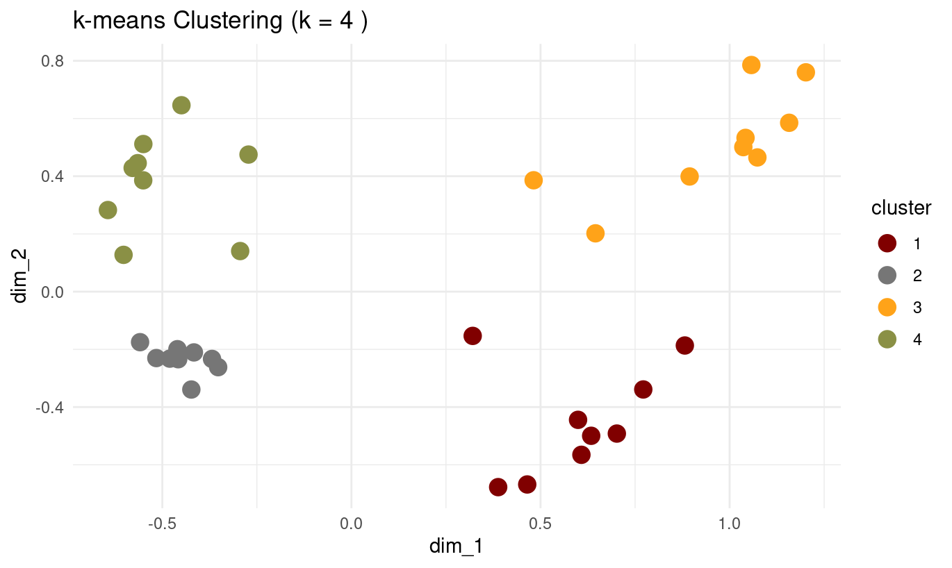
optimal_k <- 4 # Choose based on your evaluation plots
final_kmeans <- kmeans(mca_coords[, 1:2], centers = optimal_k, nstart = 25)
# Visualize final clustering
mca_coords |>
mutate(cluster = as.factor(final_kmeans$cluster)) |>
ggplot(aes(dim_1, dim_2, colour = cluster)) +
geom_point(size = 4) +
ggtitle(paste("k-means Clustering (k =", optimal_k, ")")) +
theme_minimal() +
ggsci::scale_colour_uchicago()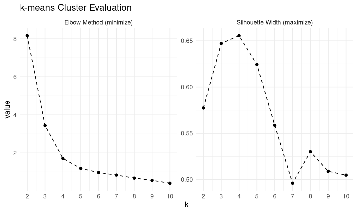
Quick Study Questions:
- What does
crossing(k = 2:10)create? - Why do we use
map2()in the clustering step? - What are the two evaluation methods being calculated?
Step 2: Apply to K-medoids (15 minutes)
Your Task: Adapt the k-means template for k-medoids clustering.
Key differences to implement:
- Use
pam(.x, k = .y)instead ofkmeans() - Extract clusters with
.y$clusteringinstead of.y$cluster - Replace
broom::glance(.x)with:r ~ tibble( tot.withinss = .x$objective[2], # Total cost from PAM k = .x$k )
Questions after running:
- What optimal k do the elbow and silhouette methods suggest?
- How do k-medoids results compare to k-means?
Step 3: Apply to K-means++ (10 minutes)
Your Task: Modify the template for enhanced k-means with better initialization.
Key change:
kmeans_result = map2(
  data,
  k,
  ~ kmeans(.x, centers = .y, algorithm = "Lloyd", iter.max = 1000, nstart = 25)
)
Questions:
- Do you notice differences in stability compared to basic k-means?
- Does the optimal k suggestion change?
Step 4: Compare All Three Methods (10 minutes)
Create final clusterings using your chosen optimal k for all three methods:
# Compare all three with optimal k
set.seed(123)
optimal_k <- 4 # Use your chosen k

# k-means
kmeans_clusters <- kmeans(
  mca_coords[, 1:2],
  centers = optimal_k,
  nstart = 25
)$cluster

# k-medoids
kmedoids_clusters <- pam(mca_coords[, 1:2], k = optimal_k)$clustering

# k-means++ (enhanced)
kmeans_plus_clusters <- kmeans(
  mca_coords[, 1:2],
  centers = optimal_k,
  algorithm = "Lloyd",
  iter.max = 1000,
  nstart = 25
)$cluster

# Create comparison plots

p1 <- mca_coords |>
  mutate(cluster = as.factor(kmeans_clusters)) |>
  ggplot(aes(dim_1, dim_2, colour = cluster)) +
  geom_point(size = 3) +
  ggtitle("k-means") +
  theme_minimal() +
  ggsci::scale_colour_uchicago()

p2 <- mca_coords |>
  mutate(cluster = as.factor(kmedoids_clusters)) |>
  ggplot(aes(dim_1, dim_2, colour = cluster)) +
  geom_point(size = 3) +
  ggtitle("k-medoids") +
  theme_minimal() +
  ggsci::scale_colour_uchicago()

p3 <- mca_coords |>
  mutate(cluster = as.factor(kmeans_plus_clusters)) |>
  ggplot(aes(dim_1, dim_2, colour = cluster)) +
  geom_point(size = 3) +
  ggtitle("k-means++") +
  theme_minimal() +
  ggsci::scale_colour_uchicago()

p1 + p2 + p3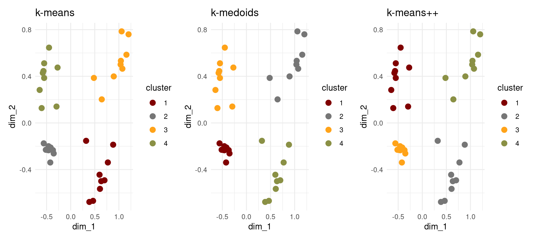
Discussion Questions:
- Which evaluation method (elbow vs silhouette) was most reliable across algorithms?
- Which clustering algorithm produced the best results for this dataset?
- What are the key trade-offs between the three methods?
Part 3: DBSCAN - Density-Based Clustering (30 minutes)
DBSCAN is fundamentally different:
- No need to specify k
- Finds arbitrary shapes
- Identifies noise points
- Key parameters:
eps(neighborhood radius) andminPts(minimum points)
Task 4: Basic DBSCAN
# Start with reasonable parameters
db_result <- dbscan(mca_coords[, 1:2], eps = 0.25, minPts = 5)

# Check results
cat("Clusters found:", max(db_result$cluster), "\n")
cat("Noise points:", sum(db_result$cluster == 0), "\n")

# Visualize
mca_coords_db <- mca_coords |>
  mutate(cluster = as.factor(db_result$cluster))

clustered_points <- mca_coords_db |> filter(cluster != "0")
noise_points <- mca_coords_db |> filter(cluster == "0")

ggplot() +
  geom_point(
    data = clustered_points,
    aes(dim_1, dim_2, color = cluster),
    size = 4
  ) +
  geom_point(
    data = noise_points,
    aes(dim_1, dim_2),
    color = "black",
    size = 2,
    shape = 4
  ) +
  labs(title = "DBSCAN Clustering", caption = "X marks indicate noise points") +
  theme_minimal() +
  ggsci::scale_colour_uchicago()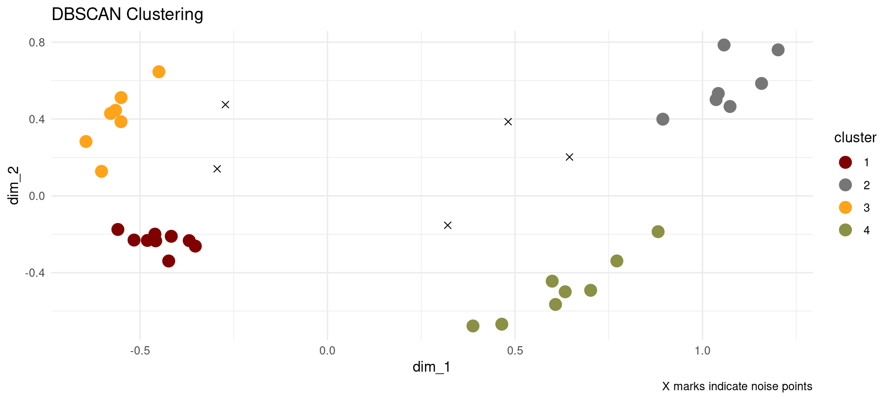
Task 5: Experiment with Epsilon
Try different eps values: c(0.1, 0.2, 0.3, 0.4, 0.5) and observe:
Key Questions:
- How does changing epsilon affect cluster formation?
- What happens to noise points as epsilon changes?
- Should all points belong to a cluster?
- Which epsilon value seems most appropriate?
Task 6: Final Comparison
Create side-by-side plots comparing your best k-means, k-medoids, and DBSCAN results.
Discussion Questions:
- Which method captures the structure of your data best?
- When would you choose DBSCAN over k-means/k-medoids?
- What are the advantages of identifying noise points?
Summary Discussion
Reflect on:
- Which clustering method worked best for this dataset and why?
- How important was the choice of evaluation method?
- What are the key considerations when choosing clustering algorithms?
- When might you prefer density-based over centroid-based methods?
Key Takeaways
- Template approach: Similar code patterns work across clustering methods
- Evaluation matters: Elbow and silhouette can give different suggestions
- No universal best: Choice depends on data characteristics and goals
- DBSCAN advantages: Handles noise and arbitrary shapes, no k required
Homework Challenge
Apply these clustering methods to a dataset from your own field. Which method works best and why?