
✅ LSE DS202W 2025/2026: Week 08 - Solutions
This solution file follows the format of a Jupyter Notebook file .ipynb you had to fill in during the lab session.
Week 8 Labs - Clustering Analysis in Python (DS202)
Overview (90 minutes total)
Today we’ll explore different clustering algorithms and evaluation methods using Multiple Correspondence Analysis (MCA) coordinates. We’ll compare k-means variants, k-medoids, and DBSCAN clustering approaches.
Technical Skills: Implement k-means, k-medoids, and DBSCAN algorithms with evaluation methods (elbow, silhouette) and adapt code templates across different clustering approaches
Analytical Skills: Compare clustering methods, evaluate their appropriateness for datasets, and interpret metrics to determine optimal cluster numbers and trade-offs
Critical Thinking: Justify algorithm selection based on data characteristics, assess outlier treatment decisions, and critique clustering limitations
Practical Application: Design complete clustering workflows, troubleshoot parameter selection challenges, and communicate results through effective visualizations
Lab Structure:
- 10 min: Clustering algorithms overview + k-means template
- 50 min: Student exploration of algorithms and evaluation methods
- 30 min: DBSCAN exploration
Part 1: Introduction to Clustering Algorithms (10 minutes)
Key Differences Between Clustering Methods
| Algorithm | Centers | Distance | Outlier Sensitivity | Use Case |
|---|---|---|---|---|
| k-means | Computed centroids | Euclidean | High | Spherical clusters |
| k-means++ | Smart initialization | Euclidean | High | Better initial centroids |
| k-medoids | Actual data points | Any metric | Low | Non-spherical clusters |
| DBSCAN | None (density-based) | Any metric | Very low | Arbitrary shapes |
⚙️ Setup
Downloading the student solutions
Click on the below button to download the student notebook.
Loading libraries
import pandas as pd
import numpy as np
import matplotlib.pyplot as plt
import seaborn as sns
from sklearn.cluster import KMeans, DBSCAN
from sklearn.metrics import silhouette_score, silhouette_samples
import kmedoids
from sklearn.preprocessing import StandardScaler
from scipy.spatial.distance import pdist, squareform
from sklearn.metrics import pairwise_distances
import warnings

warnings.filterwarnings("ignore")

# Load the MCA coordinates from Week 7
mca_coords = pd.read_csv("data/mca-week-7.csv")

# If you have the actual MCA data file, uncomment the line below:
# mca_coords = pd.read_csv("data/mca-week-7.csv")

print(f"Data shape: {mca_coords.shape}")
print(mca_coords.head())
Data shape: (36, 3)
dim_1 dim_2 category
0 -0.558831 -0.175055 avoid_transport_fare_n
1 0.645299 0.202141 avoid_transport_fare_y
2 -0.416500 -0.210573 stealing_property_n
3 1.157445 0.585178 stealing_property_y
4 -0.515787 -0.230177 cheating_taxes_nPart 2: K-means Template & Algorithm Applications (50 minutes)
Step 1: Study the K-means Template (15 minutes)
Here’s the complete workflow for k-means clustering evaluation:
# Set random seed for reproducibility
np.random.seed(123)


def evaluate_kmeans_clustering(data, k_range=range(2, 11)):
    """
    Evaluate k-means clustering using elbow method and silhouette analysis
    """
    results = []

    for k in k_range:
        # Fit k-means
        kmeans = KMeans(n_clusters=k, random_state=123, n_init=25, init='random')
        labels = kmeans.fit_predict(data)

        # Calculate metrics
        inertia = kmeans.inertia_  # Within-cluster sum of squares
        silhouette_avg = silhouette_score(data, labels)

        results.append({"k": k, "inertia": inertia, "silhouette": silhouette_avg})

    return pd.DataFrame(results)


# Evaluate k-means clustering
X = mca_coords[["dim_1", "dim_2"]].values
kmeans_results = evaluate_kmeans_clustering(X)

# Create evaluation plots
fig, (ax1, ax2) = plt.subplots(1, 2, figsize=(12, 5))

# Elbow plot
ax1.plot(kmeans_results["k"], kmeans_results["inertia"], "bo-")
ax1.set_xlabel("Number of clusters (k)")
ax1.set_ylabel("Within-cluster sum of squares")
ax1.set_title("Elbow Method (minimize)")
ax1.grid(True, alpha=0.3)

# Silhouette plot
ax2.plot(kmeans_results["k"], kmeans_results["silhouette"], "ro-")
ax2.set_xlabel("Number of clusters (k)")
ax2.set_ylabel("Average silhouette score")
ax2.set_title("Silhouette Analysis (maximize)")
ax2.grid(True, alpha=0.3)

plt.tight_layout()
plt.show()

print("K-means evaluation results:")
print(kmeans_results)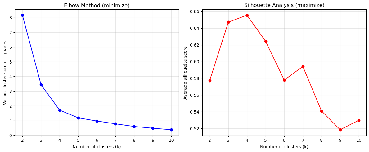
K-means evaluation results:
    k   inertia  silhouette
0   2  8.165185    0.577374
1   3  3.440244    0.647201
2   4  1.711057    0.655597
3   5  1.184902    0.624318
4   6  0.971511    0.577913
5   7  0.779726    0.594172
6   8  0.600888    0.540965
7   9  0.480704    0.518466
8 10 0.379685 0.529725Check out the yellowbrick library to see how to implement the elbow and silhouette methods in a simpler way (see for example this page)
You could also apply the silhouette and elbow methods using the yellowbrick library, which provides built-in visualizers for these evaluation methods. Check out the yellowbrick documentation.
For example, to use the elbow method with yellowbrick, you can do:
from yellowbrick.cluster import KElbowVisualizer
model = KMeans(random_state=123, n_init=25, init='random')
visualizer = KElbowVisualizer(model,force_model=True,timings=False)
visualizer.fit(X)
visualizer.show()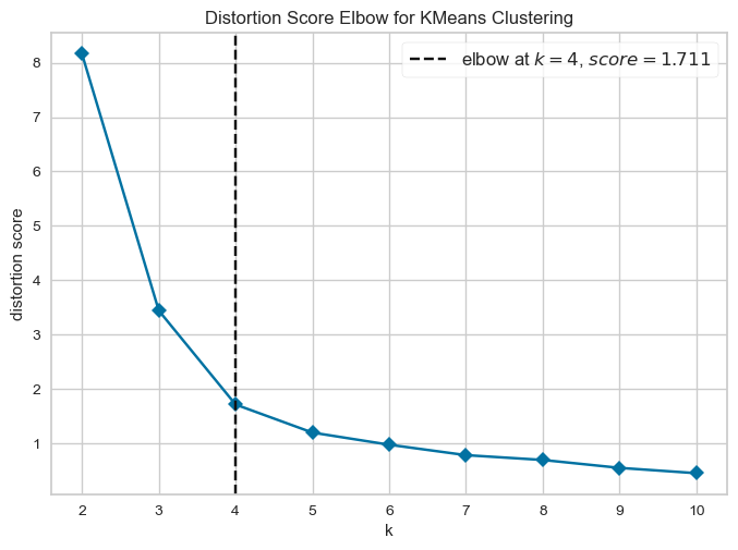
For silhouette analysis, you can use:
from yellowbrick.cluster import KElbowVisualizer

model = KMeans(random_state=123, n_init=25, init='random')
visualizer = KElbowVisualizer(model, metric='silhouette', force_model=True, timings=False)
visualizer.fit(X)
visualizer.show()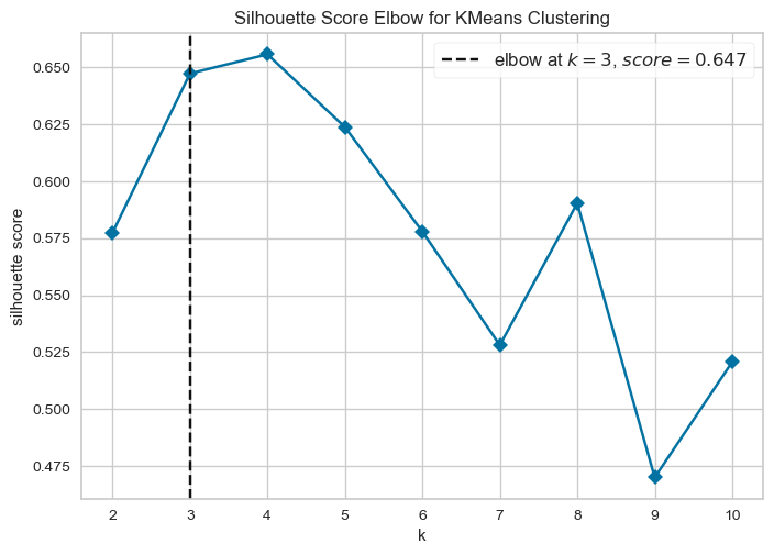
# Create final clustering with chosen k
optimal_k = 4  # Choose based on your evaluation plots

# Fit final k-means model
final_kmeans = KMeans(n_clusters=optimal_k, random_state=123, n_init=25, init='random')
kmeans_labels = final_kmeans.fit_predict(X)

# Visualize final clustering
plt.figure(figsize=(8, 6))
colors = ['red', 'blue', 'green', 'orange', 'purple', 'brown', 'pink', 'gray', 'olive', 'cyan']
for i in range(optimal_k):
    mask = kmeans_labels == i
    plt.scatter(mca_coords.loc[mask, 'dim_1'],
               mca_coords.loc[mask, 'dim_2'],
               c=colors[i],
               label=f'Cluster {i+1}',
               s=60,
               alpha=0.7)

plt.xlabel('Dimension 1')
plt.ylabel('Dimension 2')
plt.title(f'K-means Clustering (k = {optimal_k})')
plt.legend()
plt.grid(True, alpha=0.3)
plt.show()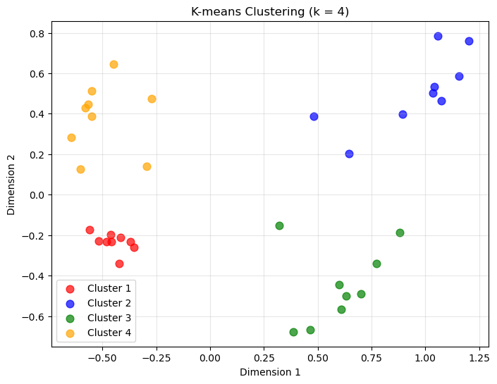
Quick Study Questions:
- What does the range(2, 11) create in our evaluation?
- Why do we use multiple random initializations (n_init=25)?
- What are the two evaluation methods being calculated?
What does range(2, 11) create in our evaluation?
range(2, 11) generates the sequence:
\[ 2, 3, 4, 5, 6, 7, 8, 9, 10 \]
This means the clustering algorithm is run multiple times, each time with a different number of clusters \(k\).
The goal is to evaluate how clustering quality changes as we vary \(k\). For each value of \(k\), we compute evaluation metrics and then compare the results.
We start at 2 clusters because clustering with \(k=1\) is not meaningful (all observations would belong to the same cluster). The upper bound of 10 simply provides a reasonable range to explore without making computation too expensive.
Why do we use multiple random initializations (n_init=25)?
Algorithms like K-means start with random initial cluster centres.
Because of this, the algorithm may converge to different local optima depending on the initial starting positions.
Running the algorithm multiple times with different initializations:
- increases the chance of finding a better clustering solution
- reduces the risk of obtaining a poor result caused by unlucky starting points
n_init=25 means the algorithm is run 25 times, and the best solution (lowest clustering cost) is retained.
What are the two evaluation methods being calculated?
The code computes two commonly used clustering evaluation metrics.
1. Elbow method (total within-cluster distance / inertia)
This metric measures how compact the clusters are. Specifically, it calculates the total within-cluster distance between observations and their assigned cluster centre.
For clustering methods like K-means, the objective function (often called inertia) is:
\[ W(k) = \sum_{j=1}^{k} \sum_{i \in C_j} | x_i - \mu_j |^2 \]
where:
- \(k\) = number of clusters
- \(C_j\) = set of observations in cluster \(j\)
- \(x_i\) = observation \(i\)
- \(\mu_j\) = centroid of cluster \(j\)
- \(|x_i - \mu_j|^2\) = squared distance between the observation and its cluster centre
In words, this sums the squared distances between each observation and the centre of the cluster it belongs to.
As the number of clusters \(k\) increases:
- clusters become smaller and more compact
- the total within-cluster distance decreases
However, the improvement eventually slows down. When plotted against \(k\), the point where the curve starts to flatten is called the elbow, and it suggests a reasonable number of clusters.
For k-medoids, the idea is the same, but the cluster centre is a medoid (an actual observation) rather than a centroid. The objective function becomes the sum of distances between each observation and its assigned medoid.
2. Silhouette score
The silhouette score measures how well observations fit within their assigned cluster compared to neighbouring clusters.
For each observation (i):
- \(a(i)\) = average distance to other points in the same cluster
- \(b(i)\) = average distance to points in the nearest neighbouring cluster
The silhouette value for each observation is
\[ s(i)=\frac{b(i)-a(i)}{\max(a(i),b(i))} \]
Values range from −1 to 1:
| Score | Interpretation |
|---|---|
| close to 1 | observation fits its cluster well |
| around 0 | clusters overlap |
| negative | observation may be misclassified |
In our evaluation, we compute the silhouette score for every observation and then take the average.
We then plot the average silhouette score for each value of (k). The best number of clusters is typically the (k) that maximizes the average silhouette score.
Why use both methods?
The elbow method focuses on cluster compactness, while the silhouette score evaluates how well clusters are separated. Using both gives a more reliable indication of the appropriate number of clusters.
Step 2: Apply to K-means++ (10 minutes)
Your Task: Modify the template for enhanced k-means with better initialization.
Key change: K-means++ initialization is actually the default in scikit-learn’s KMeans!
def evaluate_kmeans_plus_clustering(data, k_range=range(2, 11)):
    """
    Evaluate k-means++ clustering (with explicit k-means++ initialization)
    """
    results = []

    for k in k_range:
        # Fit k-means with explicit k-means++ initialization
        kmeans_plus = KMeans(n_clusters=k,
                           init='k-means++',  # Explicit k-means++ initialization
                           random_state=123,
                           n_init=25,
                           max_iter=1000)
        labels = kmeans_plus.fit_predict(data)

        # Calculate metrics
        inertia = kmeans_plus.inertia_
        silhouette_avg = silhouette_score(data, labels)

        results.append({
            'k': k,
            'inertia': inertia,
            'silhouette': silhouette_avg
        })

    return pd.DataFrame(results)

# Evaluate k-means++ clustering
kmeans_plus_results = evaluate_kmeans_plus_clustering(X)

# Create evaluation plots
fig, (ax1, ax2) = plt.subplots(1, 2, figsize=(12, 5))

# Elbow plot
ax1.plot(kmeans_plus_results['k'], kmeans_plus_results['inertia'], 'bo-')
ax1.set_xlabel('Number of clusters (k)')
ax1.set_ylabel('Within-cluster sum of squares')
ax1.set_title('K-means++ Elbow Method (minimize)')
ax1.grid(True, alpha=0.3)

# Silhouette plot
ax2.plot(kmeans_plus_results['k'], kmeans_plus_results['silhouette'], 'ro-')
ax2.set_xlabel('Number of clusters (k)')
ax2.set_ylabel('Average silhouette score')
ax2.set_title('Silhouette Analysis (maximize)')
ax2.grid(True, alpha=0.3)

plt.tight_layout()
plt.show()

print("K-means++ evaluation results:")
print(kmeans_plus_results)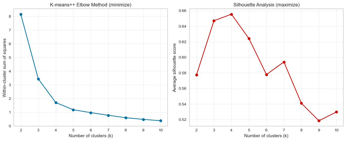
K-means++ evaluation results:
    k   inertia  silhouette
0   2  8.165185    0.577374
1   3  3.440244    0.647201
2   4  1.711057    0.655597
3   5  1.184902    0.624318
4   6  0.971511    0.577913
5   7  0.779726    0.594172
6   8  0.600888    0.540965
7   9  0.480704    0.518466
8  10  0.379685    0.529725
# Final k-means++ clustering
kmeans_plus_final = KMeans(n_clusters=optimal_k,
init='k-means++',
random_state=123,
n_init=25,
max_iter=1000)
kmeans_plus_labels = kmeans_plus_final.fit_predict(X)
# Visualize k-means++ results
plt.figure(figsize=(8, 6))
for i in range(optimal_k):
mask = kmeans_plus_labels == i
plt.scatter(mca_coords.loc[mask, 'dim_1'],
mca_coords.loc[mask, 'dim_2'],
c=colors[i],
label=f'Cluster {i+1}',
s=60,
alpha=0.7)
plt.xlabel('Dimension 1')
plt.ylabel('Dimension 2')
plt.title(f'K-means++ Clustering (k = {optimal_k})')
plt.legend()
plt.grid(True, alpha=0.3)
plt.show()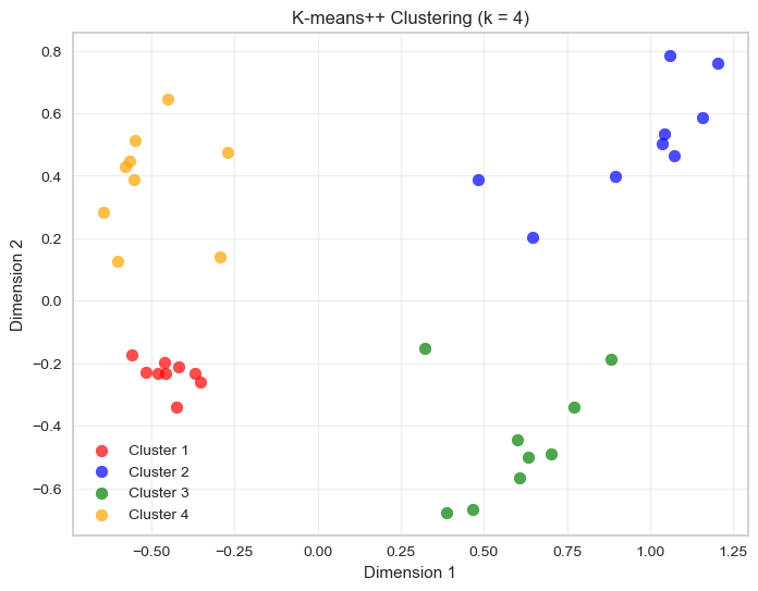
Questions:
- Do you notice differences in stability compared to basic k-means?
- Does the optimal k suggestion change?
1. Do you notice differences in stability compared to basic k-means?
In this example, no meaningful differences appear between the two results. The cluster assignments are effectively identical.
This happens because the dataset already has very clearly separated groups. When clusters are well separated, even standard k-means with random initialisation quickly converges to the same solution.
In such situations:
- different initialisations tend to converge to the same global optimum
- cluster assignments remain stable across runs
The advantage of K-means++ becomes more visible when:
- clusters overlap
- clusters have irregular shapes
- the dataset is high dimensional
- the algorithm might otherwise get stuck in poor local minima
2. Does the optimal k suggestion change?
No. The optimal number of clusters does not change.
Both the elbow method and the silhouette curve depend on the overall structure of the dataset, not on the specific initialisation used in a single run.
Since the data structure is unchanged, both methods would still suggest the same value of \(k\).
✅ Key takeaway
When clusters are well separated, different initialisation strategies often lead to the same final clustering, which is why you do not observe differences here.
Note that, since k-means++ is the default initialization method in scikit-learn’s KMeans, you may not see a difference in results if you were already using the default settings. However, explicitly setting init='k-means++' ensures that you are using the improved initialization method, which can lead to better convergence and more consistent results across runs.
If you were to replace the line python kmeans_plus = KMeans(n_clusters=k,init='k-means++',random_state=123, n_init=25,max_iter=1000) in your code with python kmeans_plus = KMeans(n_clusters=k, random_state=123, n_init=25'), you would still be using k-means++ initialization, since it is the default. However, explicitly specifying it can help clarify your intentions and ensure that you are indeed using the improved initialization method.
Step 3: Apply to k-medoids (10 min)
Your Task: Adapt the k-means template for k-medoids clustering.
💡 Hint: Use the kmedoids library for your code (see documentation)
def evaluate_kmedoids_clustering(data, k_range=range(2, 11)):
    """
    Evaluate k-medoids clustering using cost and silhouette analysis
    """

    # Compute distance matrix once (required by kmedoids)
    D = pairwise_distances(data)

    results = []

    for k in k_range:
        # Fit k-medoids (FasterPAM algorithm)
        result = kmedoids.fasterpam(D, k)

        labels = result.labels

        # Calculate metrics
        cost = result.loss  # Total cost (sum of distances to medoids)
        silhouette_avg = silhouette_score(data, labels)

        results.append({
            'k': k,
            'cost': cost,
            'silhouette': silhouette_avg
        })

    return pd.DataFrame(results)

# Evaluate k-medoids clustering
kmedoids_results = evaluate_kmedoids_clustering(X)

# Create evaluation plots
fig, (ax1, ax2) = plt.subplots(1, 2, figsize=(12, 5))

# Cost plot (similar to elbow)
ax1.plot(kmedoids_results['k'], kmedoids_results['cost'], 'bo-')
ax1.set_xlabel('Number of clusters (k)')
ax1.set_ylabel('Total cost')
ax1.set_title('K-medoids Cost Method (minimize)')
ax1.grid(True, alpha=0.3)

# Silhouette plot
ax2.plot(kmedoids_results['k'], kmedoids_results['silhouette'], 'ro-')
ax2.set_xlabel('Number of clusters (k)')
ax2.set_ylabel('Average silhouette score')
ax2.set_title('Silhouette Analysis (maximize)')
ax2.grid(True, alpha=0.3)

plt.tight_layout()
plt.show()

print("K-medoids evaluation results:")
print(kmedoids_results)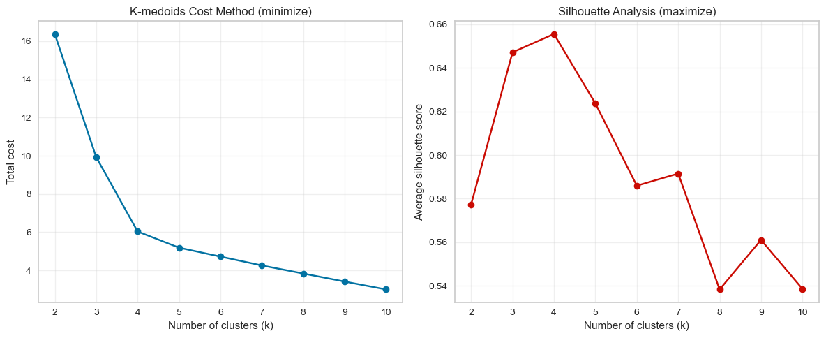
K-medoids evaluation results:
    k       cost  silhouette
0   2  16.375313    0.577374
1   3   9.929361    0.647201
2   4   6.037396    0.655597
3   5   5.189930    0.623720
4   6   4.723066    0.585956
5   7   4.258115    0.591514
6   8   3.837101    0.538308
7   9   3.414389    0.561052
8 10 3.003361 0.538553Unlike k-means, the kmedoids library operates on a distance matrix rather than the raw feature matrix.
This is why we compute pairwise distances using:
pairwise_distances(data)This matrix contains the distance between every pair of observations in the dataset.
optimal_k = 4  # Choose based on your evaluation plots
# Compute distance matrix
D = pairwise_distances(X)

# Run k-medoids clustering with optimal k
kmedoids_final = kmedoids.fasterpam(D, optimal_k)

kmedoids_labels = kmedoids_final.labels
colors = sns.color_palette("magma", n_colors=max(4, optimal_k))
# Visualize k-medoids results
plt.figure(figsize=(8, 6))
for i in range(optimal_k):
mask = kmedoids_labels == i
plt.scatter(mca_coords.loc[mask, 'dim_1'],
mca_coords.loc[mask, 'dim_2'],
c=colors[i],
label=f'Cluster {i+1}',
s=60,
alpha=0.7)
# Mark medoids
medoids_indices = kmedoids_final.medoids
medoids = X[medoids_indices]
plt.scatter(medoids[:, 0], medoids[:, 1],
c='black', marker='x', s=200, linewidths=3, label='Medoids')
plt.xlabel('Dimension 1')
plt.ylabel('Dimension 2')
plt.title(f'K-medoids Clustering (k = {optimal_k})')
plt.legend()
plt.grid(True, alpha=0.3)
plt.show()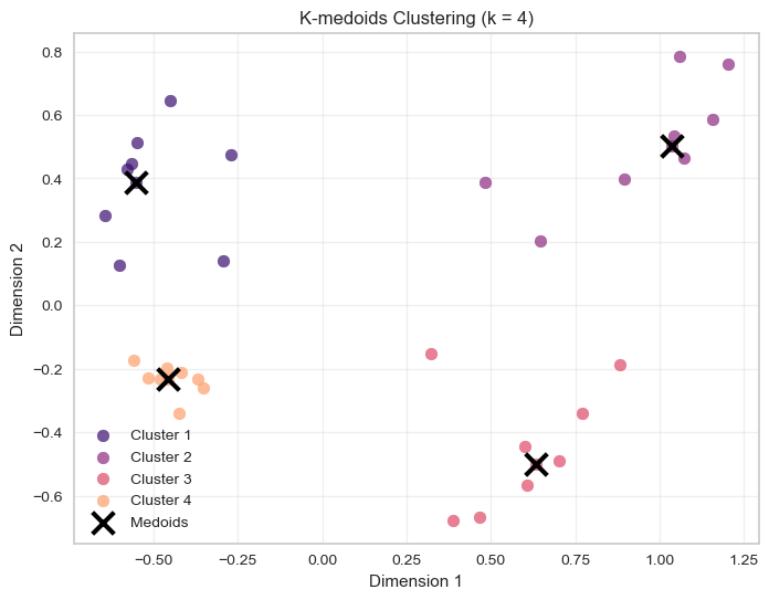
In k-means, clusters are represented by centroids (the mean of cluster observations).
In k-medoids, clusters are represented by medoids, which are actual observations from the dataset.
Because of this, k-medoids is typically more robust to outliers: extreme values cannot pull the cluster centre away from the main data cloud.
Key differences implemented:
- Use the
kmedoidslibrary instead ofKMeans - Compute a distance matrix before running the algorithm
- Extract clusters with
result.labels - Use
result.lossfor the total clustering cost - Mark actual medoid observations on the plot
Questions:
- What optimal \(k\) do the cost and silhouette methods suggest?
- How do k-medoids results compare to k-means?
1. What optimal \(k\) do the cost and silhouette methods suggest?
The two evaluation methods point to \(k = 4\) as the optimal number of clusters.
Cost method (elbow): The total cost decreases sharply between \(k = 2\) and \(k = 4\), after which the improvement becomes much smaller. This creates a clear elbow around \(k = 4\), suggesting that adding more clusters beyond this point yields diminishing returns.
Silhouette analysis: The average silhouette score reaches its maximum at \(k = 4\) (around 0.65). This indicates that clusters are most compact and well separated when the data are divided into four groups.
Taken together, both methods consistently suggest four clusters as the most appropriate choice.
2. How do k-medoids results compare to k-means?
The clustering results are very similar to those obtained with k-means.
Both methods identify the same four natural groups in the data, which indicates that the cluster structure is strong and clearly separated. The main conceptual difference lies in how cluster centres are defined:
- K-means represents each cluster using a centroid (the mean of the cluster points).
- K-medoids represents each cluster using a medoid, which is an actual observation from the dataset.
Because of this, k-medoids is typically more robust to outliers, since extreme points cannot pull the cluster centre away from the data cloud.
In this dataset, however, the clusters are well separated and contain no strong outliers, so both algorithms produce nearly identical cluster assignments.
Step 4: Compare All Three Methods (10 minutes)
Create final clusterings using your chosen optimal k for all three methods:
# Create comparison plots
fig, axes = plt.subplots(1, 3, figsize=(18, 5))

# K-means plot
for i in range(optimal_k):
    mask = kmeans_labels == i
    axes[0].scatter(mca_coords.loc[mask, 'dim_1'],
                   mca_coords.loc[mask, 'dim_2'],
                   c=colors[i],
                   label=f'Cluster {i+1}',
                   s=60,
                   alpha=0.7)
axes[0].set_title('K-means')
axes[0].set_xlabel('Dimension 1')
axes[0].set_ylabel('Dimension 2')
axes[0].grid(True, alpha=0.3)
axes[0].legend()

# K-medoids plot
for i in range(optimal_k):
    mask = kmedoids_labels == i
    axes[1].scatter(mca_coords.loc[mask, 'dim_1'],
                   mca_coords.loc[mask, 'dim_2'],
                   c=colors[i],
                   label=f'Cluster {i+1}',
                   s=60,
                   alpha=0.7)
# Mark medoids
axes[1].scatter(medoids[:, 0], medoids[:, 1],
               c='black', marker='x', s=200, linewidths=3, label='Medoids')
axes[1].set_title('K-medoids')
axes[1].set_xlabel('Dimension 1')
axes[1].set_ylabel('Dimension 2')
axes[1].grid(True, alpha=0.3)
axes[1].legend()

# K-means++ plot
for i in range(optimal_k):
    mask = kmeans_plus_labels == i
    axes[2].scatter(mca_coords.loc[mask, 'dim_1'],
                   mca_coords.loc[mask, 'dim_2'],
                   c=colors[i],
                   label=f'Cluster {i+1}',
                   s=60,
                   alpha=0.7)
axes[2].set_title('K-means++')
axes[2].set_xlabel('Dimension 1')
axes[2].set_ylabel('Dimension 2')
axes[2].grid(True, alpha=0.3)
axes[2].legend()

plt.tight_layout()
plt.show()

# Compare silhouette scores
print("Comparison of silhouette scores:")
print(f"K-means: {silhouette_score(X, kmeans_labels):.3f}")
print(f"K-medoids: {silhouette_score(X, kmedoids_labels):.3f}")
print(f"K-means++: {silhouette_score(X, kmeans_plus_labels):.3f}")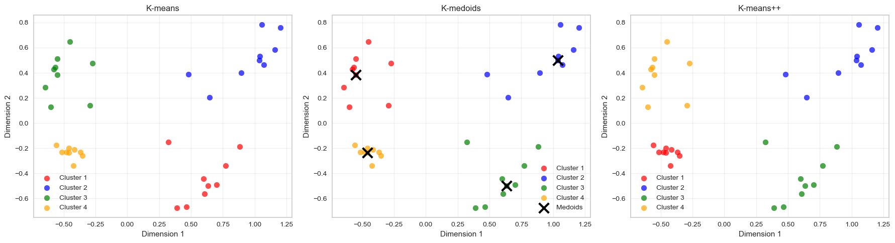
Comparison of silhouette scores:
K-means: 0.656
K-medoids: 0.656
K-means++: 0.656
Discussion Questions:
- Which evaluation method (elbow vs silhouette) was most reliable across algorithms?
- Which clustering algorithm produced the best results for this dataset?
- What are the key trade-offs between the three methods?
1. Which evaluation method (elbow vs silhouette) was most reliable across algorithms?
The silhouette method was the most reliable across the three algorithms.
Across k-means, k-means++, and k-medoids, the silhouette score consistently peaks at (k = 4). This indicates that the clusters are most well separated and internally cohesive when the data are divided into four groups.
The elbow method also suggests (k ), but the elbow is somewhat less sharply defined. The curve gradually flattens after (k = 4), which makes the exact turning point slightly more subjective to interpret.
Because the silhouette score provides a clear maximum, it offers a more unambiguous recommendation in this case.
2. Which clustering algorithm produced the best results for this dataset?
All three algorithms produce very similar clustering results for this dataset.
The clusters are well separated in the feature space, which means that:
- K-means
- K-means++
- K-medoids
all recover essentially the same four clusters.
However, k-means++ is generally preferable in practice, because its improved initialization tends to produce more stable results and faster convergence than basic k-means.
In this dataset, though, the cluster structure is so clear that all three methods perform equally well.
3. What are the key trade-offs between the three methods?
| Method | Strengths | Limitations |
|---|---|---|
| K-means | Fast and scalable for large datasets | Sensitive to initialization and outliers |
| K-means++ | Better initialization improves stability and convergence | Still sensitive to outliers |
| K-medoids | More robust to outliers because centres are real observations | Computationally more expensive |
Key conceptual differences:
- K-means / k-means++ represent clusters using centroids (means).
- K-medoids represent clusters using actual data points (medoids).
Because of this, k-medoids is more robust, but k-means-based methods are typically faster and more scalable.
✅ Overall takeaway
For this dataset:
- The silhouette method clearly identifies (k = 4).
- All three algorithms recover the same cluster structure.
- In practice, k-means++ is often preferred because it combines speed with improved initialization stability.
Part 3: DBSCAN - Density-Based Clustering (30 minutes)
DBSCAN is fundamentally different:
- No need to specify k
- Finds arbitrary shapes
- Identifies noise points
- Key parameters:
eps(neighborhood radius) andmin_samples(minimum points)
Task 4: Basic DBSCAN
# Start with reasonable parameters
dbscan = DBSCAN(eps=0.5, min_samples=5)
dbscan_labels = dbscan.fit_predict(X)

# Check results
n_clusters = len(set(dbscan_labels)) - (1 if -1 in dbscan_labels else 0)
n_noise = list(dbscan_labels).count(-1)

print(f"Clusters found: {n_clusters}")
print(f"Noise points: {n_noise}")
print(f"Cluster labels: {np.unique(dbscan_labels)}")
Clusters found: 2
Noise points: 0
Cluster labels: [0 1]# Visualize DBSCAN results
plt.figure(figsize=(10, 6))
# Plot clustered points
for i in range(n_clusters):
mask = dbscan_labels == i
plt.scatter(mca_coords.loc[mask, 'dim_1'],
mca_coords.loc[mask, 'dim_2'],
c=colors[i % len(colors)],
label=f'Cluster {i+1}',
s=60,
alpha=0.7)
# Plot noise points
if n_noise > 0:
noise_mask = dbscan_labels == -1
plt.scatter(mca_coords.loc[noise_mask, 'dim_1'],
mca_coords.loc[noise_mask, 'dim_2'],
c='black',
marker='x',
s=60,
label='Noise',
alpha=0.8)
plt.xlabel('Dimension 1')
plt.ylabel('Dimension 2')
plt.title(f'DBSCAN Clustering (eps=0.5, min_samples=5)')
plt.legend()
plt.grid(True, alpha=0.3)
plt.show()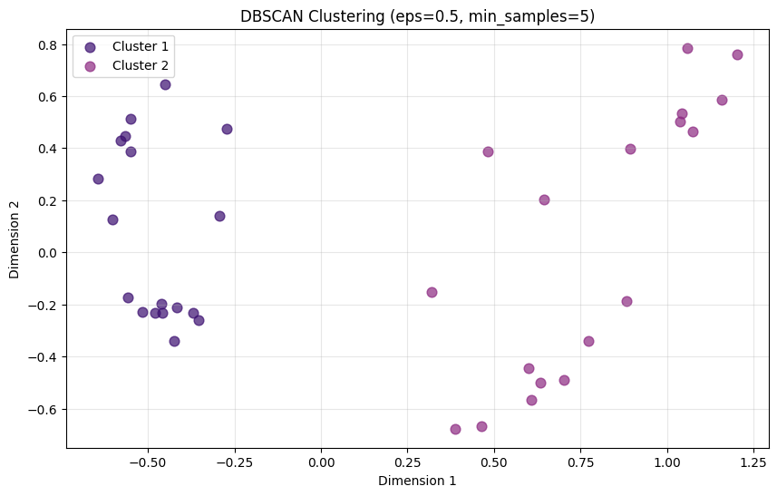
Task 5: Experiment with Epsilon
Try different eps values and observe the effects:
# Test different epsilon values
eps_values = [0.1, 0.2, 0.3, 0.5, 0.7, 1.0]
dbscan_results = []

for eps in eps_values:
    dbscan = DBSCAN(eps=eps, min_samples=5)
    labels = dbscan.fit_predict(X)

    n_clusters = len(set(labels)) - (1 if -1 in labels else 0)
    n_noise = list(labels).count(-1)

    # Calculate silhouette score (only if we have clusters and not all points are noise)
    if n_clusters > 1 and n_noise < len(X) - 1:
        # Remove noise points for silhouette calculation
        mask = labels != -1
        if np.sum(mask) > 1 and len(np.unique(labels[mask])) > 1:
            silhouette_avg = silhouette_score(X[mask], labels[mask])
        else:
            silhouette_avg = -1
    else:
        silhouette_avg = -1

    dbscan_results.append({
        'eps': eps,
        'n_clusters': n_clusters,
        'n_noise': n_noise,
        'silhouette': silhouette_avg
    })

dbscan_df = pd.DataFrame(dbscan_results)
print("DBSCAN parameter exploration:")
print(dbscan_df)
DBSCAN parameter exploration:
eps n_clusters n_noise silhouette
0 0.1 1 28 -1.000000
1 0.2 4 8 0.783289
2 0.3 4 4 0.743885
3 0.5 2 0 0.577374
4 0.7 1 0 -1.000000
5 1.0 1 0 -1.000000The silhouette score measures how well observations fit within their assigned cluster compared to neighbouring clusters.
For each observation \(i\):
\[ s(i) = \frac{b(i) - a(i)}{\max(a(i), b(i))} \]
where:
- \(a(i)\) = average distance to points in the same cluster
- \(b(i)\) = average distance to points in the nearest neighbouring cluster
The score ranges from −1 to 1:
| Score | Interpretation |
|---|---|
| ≈ 1 | well separated clusters |
| ≈ 0 | overlapping clusters |
| < 0 | possible misclassification |
However, this metric was originally designed for algorithms such as k-means, where every observation belongs to a cluster.
With DBSCAN, some observations are labelled as noise (label = -1). Because noise points do not belong to any cluster, we exclude them from the silhouette calculation. This means the silhouette score evaluates only the clustered observations, not the full dataset.
In addition, silhouette scores rely on distance-based cluster separation, while DBSCAN identifies clusters as regions of high density. As a result, silhouette scores may not always reflect the quality of density-based clusters.
For density-based clustering, alternative evaluation metrics such as the Density-Based Clustering Validation (DBCV) index can sometimes be more appropriate, as they explicitly account for density connectedness within clusters and density separation between clusters.
In practice, it is therefore helpful to evaluate DBSCAN results using multiple diagnostics, including silhouette scores, the number of clusters, the number of noise points, and visual inspection of the clustering structure.
One metric designed specifically for density-based clustering is the Density-Based Clustering Validation (DBCV) index.
Unlike the silhouette score, which relies purely on distance-based cluster separation, DBCV evaluates clustering quality using:
- density connectedness within clusters
- density separation between clusters
This makes it more closely aligned with the logic of DBSCAN, where clusters are defined as dense regions separated by sparse areas.
You can compute DBCV alongside the other diagnostics in the parameter exploration loop.
from hdbscan.validity import validity_index

# Test different epsilon values
eps_values = [0.1, 0.2, 0.3, 0.5, 0.7, 1.0]
dbscan_results = []

for eps in eps_values:

    dbscan = DBSCAN(eps=eps, min_samples=5)
    labels = dbscan.fit_predict(X)

    n_clusters = len(set(labels)) - (1 if -1 in labels else 0)
    n_noise = list(labels).count(-1)

    # Silhouette score (excluding noise points)
    if n_clusters > 1 and n_noise < len(X) - 1:
        mask = labels != -1
        if np.sum(mask) > 1 and len(np.unique(labels[mask])) > 1:
            silhouette_avg = silhouette_score(X[mask], labels[mask])
        else:
            silhouette_avg = np.nan
    else:
        silhouette_avg = np.nan

    # DBCV score
    if n_clusters > 1:
        try:
            dbcv_score = validity_index(X, labels)
        except:
            dbcv_score = np.nan
    else:
        dbcv_score = np.nan

    dbscan_results.append({
        "eps": eps,
        "n_clusters": n_clusters,
        "n_noise": n_noise,
        "silhouette": silhouette_avg,
        "dbcv": dbcv_score
    })

dbscan_df = pd.DataFrame(dbscan_results)
print(dbscan_df)
This produces a table comparing cluster structure across epsilon values.
Example output (for our dataset):
   eps  n_clusters  n_noise  silhouette      dbcv
0  0.1           1       28         NaN       NaN
1  0.2           4        8    0.783289  0.636490
2  0.3           4        4    0.743885  0.684109
3  0.5           2        0    0.577374  0.617488
4  0.7           1        0         NaN       NaN
5  1.0           1        0         NaN       NaN
⚠️ Important: DBCV can only be computed when at least two clusters are detected (excluding noise). If DBSCAN returns only one cluster or labels most observations as noise, the score cannot be calculated and will appear as NaN.
In practice, DBSCAN results are usually evaluated using several diagnostics together, including:
- silhouette score (excluding noise points)
- DBCV score
- number of clusters detected
- number of noise points
- visual inspection of the clustering structure
# Visualize effect of different epsilon values
fig, axes = plt.subplots(2, 3, figsize=(18, 10))
axes = axes.ravel()

for idx, eps in enumerate(eps_values):
    dbscan = DBSCAN(eps=eps, min_samples=5)
    labels = dbscan.fit_predict(X)

    n_clusters = len(set(labels)) - (1 if -1 in labels else 0)
    n_noise = list(labels).count(-1)

    # Plot clusters
    for i in range(n_clusters):
        mask = labels == i
        axes[idx].scatter(mca_coords.loc[mask, 'dim_1'],
                         mca_coords.loc[mask, 'dim_2'],
                         c=colors[i % len(colors)],
                         s=30,
                         alpha=0.7)

    # Plot noise
    if n_noise > 0:
        noise_mask = labels == -1
        axes[idx].scatter(mca_coords.loc[noise_mask, 'dim_1'],
                         mca_coords.loc[noise_mask, 'dim_2'],
                         c='black',
                         marker='x',
                         s=30,
                         alpha=0.8)

    axes[idx].set_title(f'eps={eps}\nClusters: {n_clusters}, Noise: {n_noise}')
    axes[idx].set_xlabel('Dimension 1')
    axes[idx].set_ylabel('Dimension 2')
    axes[idx].grid(True, alpha=0.3)

plt.tight_layout()
plt.show()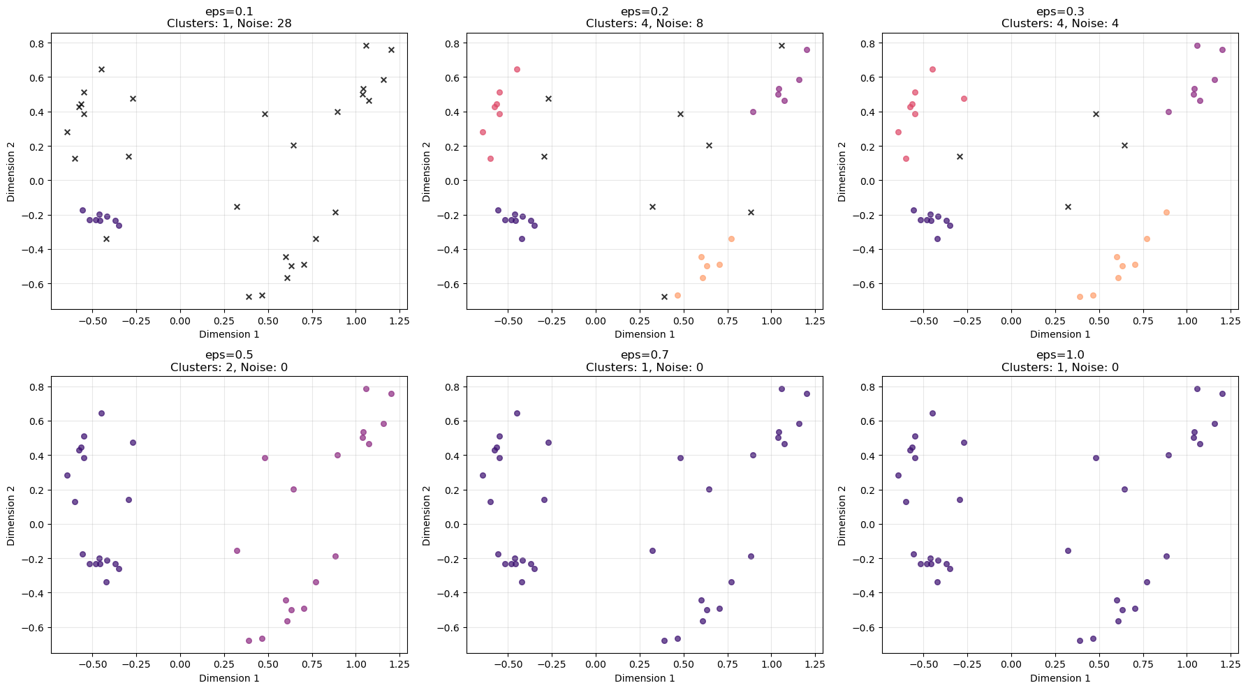
Key Questions:
- How does changing epsilon affect cluster formation?
- What happens to noise points as epsilon changes?
- Should all points belong to a cluster?
- Which epsilon value seems most appropriate?
1. How does changing epsilon affect cluster formation?
The epsilon parameter (eps) controls how close points must be to be considered neighbours, and therefore how clusters grow.
As eps increases:
Small eps (0.1) → neighbourhoods are very small
- very few points are connected
- many points are labelled as noise
Moderate eps (0.2–0.3) → clusters start forming
- nearby points become connected
- several distinct clusters appear
Large eps (0.5 and above) → neighbourhoods become large
- clusters merge together
- eventually most points belong to one large cluster
In other words:
\[ \text{larger eps} \Rightarrow \text{more connectivity between points} \]
2. What happens to noise points as epsilon changes?
Noise points decrease as epsilon increases.
From the plots:
| eps | clusters | noise |
|---|---|---|
| 0.1 | 1 | 28 |
| 0.2 | 4 | 8 |
| 0.3 | 4 | 4 |
| 0.5 | 2 | 0 |
| 0.7 | 1 | 0 |
| 1.0 | 1 | 0 |
This happens because larger eps values make it easier for points to fall within neighbourhoods, so fewer observations remain isolated.
3. Should all points belong to a cluster?
Not necessarily.
A key feature of DBSCAN is that it can identify noise or outliers.
Points that lie in low-density regions are intentionally labelled as noise rather than being forced into clusters. This is often desirable because:
- it prevents clusters from being distorted by outliers
- it highlights observations that may represent unusual cases
Therefore, it is normal and often useful for some points to remain unclustered.
4. Which epsilon value seems most appropriate?
Based on the plots, eps ≈ 0.3 appears most appropriate.
At this value:
- the algorithm detects four clear clusters, which matches the visible structure of the data
- only a small number of points remain noise
- clusters are distinct and well separated
By contrast:
- eps = 0.1 produces too much noise
- eps ≥ 0.5 merges clusters together
Thus, 0.3 provides the best balance between cluster detection and noise filtering.
✅ Takeaway
The epsilon parameter strongly influences DBSCAN results:
- too small → excessive noise
- too large → clusters merge
- moderate values → meaningful clusters emerge.
Task 6: Final Comparison
Create side-by-side plots comparing your best k-means, k-medoids, and DBSCAN results:
# Choose best DBSCAN parameters based on exploration
best_eps = 0.3  # Adjust based on your results
dbscan_final = DBSCAN(eps=best_eps, min_samples=5)
dbscan_final_labels = dbscan_final.fit_predict(X)

# Final comparison plot
fig, axes = plt.subplots(1, 4, figsize=(20, 5))

# K-means
for i in range(optimal_k):
    mask = kmeans_labels == i
    axes[0].scatter(mca_coords.iloc[mask, 0],
                   mca_coords.iloc[mask, 1],
                   c=colors[i], s=60, alpha=0.7)
axes[0].set_title('K-means')
axes[0].grid(True, alpha=0.3)

# K-medoids
for i in range(optimal_k):
    mask = kmedoids_labels == i
    axes[1].scatter(mca_coords.iloc[mask, 0],
                   mca_coords.iloc[mask, 1],
                   c=colors[i], s=60, alpha=0.7)
axes[1].scatter(medoids[:, 0], medoids[:, 1],
               c='black', marker='x', s=200, linewidths=3)
axes[1].set_title('K-medoids')
axes[1].grid(True, alpha=0.3)

# K-means++
for i in range(optimal_k):
    mask = kmeans_plus_labels == i
    axes[2].scatter(mca_coords.iloc[mask, 0],
                   mca_coords.iloc[mask, 1],
                   c=colors[i], s=60, alpha=0.7)
axes[2].set_title('K-means++')
axes[2].grid(True, alpha=0.3)

# DBSCAN
n_clusters_final = len(set(dbscan_final_labels)) - (1 if -1 in dbscan_final_labels else 0)
for i in range(n_clusters_final):
    mask = dbscan_final_labels == i
    axes[3].scatter(mca_coords.iloc[mask, 0],
                   mca_coords.iloc[mask, 1],
                   c=colors[i % len(colors)], s=60, alpha=0.7)
if -1 in dbscan_final_labels:
    noise_mask = dbscan_final_labels == -1
    axes[3].scatter(mca_coords.iloc[noise_mask, 0],
                   mca_coords.iloc[noise_mask, 1],
                   c='black', marker='x', s=60, alpha=0.8)
axes[3].set_title(f'DBSCAN (eps={best_eps})')
axes[3].grid(True, alpha=0.3)

for ax in axes:
    ax.set_xlabel('Dimension 1')
    ax.set_ylabel('Dimension 2')

plt.tight_layout()
plt.show()

# Print final comparison metrics
print("Final Clustering Comparison:")
print(f"K-means silhouette score: {silhouette_score(X, kmeans_labels):.3f}")
print(f"K-medoids silhouette score: {silhouette_score(X, kmedoids_labels):.3f}")
print(f"K-means++ silhouette score: {silhouette_score(X, kmeans_plus_labels):.3f}")

# DBSCAN silhouette (excluding noise points)
if len(set(dbscan_final_labels)) > 2 or (len(set(dbscan_final_labels)) == 2 and -1 not in dbscan_final_labels):
    mask = dbscan_final_labels != -1
    if np.sum(mask) > 1 and len(np.unique(dbscan_final_labels[mask])) > 1:
        dbscan_silhouette = silhouette_score(X[mask], dbscan_final_labels[mask])
        print(f"DBSCAN silhouette score: {dbscan_silhouette:.3f}")
    else:
        print("DBSCAN silhouette score: Not applicable (insufficient clusters)")
else:
    print("DBSCAN silhouette score: Not applicable (insufficient clusters)")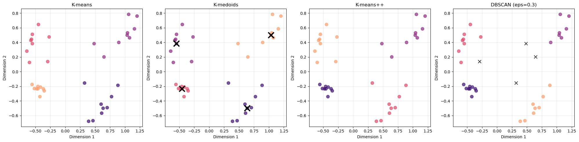
Final Clustering Comparison:
K-means silhouette score: 0.656
K-medoids silhouette score: 0.656
K-means++ silhouette score: 0.656
DBSCAN silhouette score: 0.744
Discussion Questions:
- Which method captures the structure of your data best?
- When would you choose DBSCAN over k-means/k-medoids?
- What are the advantages of identifying noise points?
1. Which method captures the structure of your data best?
All methods recover the same four main groups, indicating that the cluster structure is strong and well separated.
However, DBSCAN appears to capture the structure slightly better in this case:
- It achieves the highest silhouette score (0.744) compared to 0.656 for the other methods.
- It identifies several points as noise, rather than forcing them into clusters.
The other algorithms:
- K-means
- K-medoids
- K-means++
assign every observation to a cluster, which can sometimes lead to slightly less natural groupings when outliers are present.
2. When would you choose DBSCAN over k-means/k-medoids?
DBSCAN is preferable when:
1. The number of clusters is unknown
Unlike k-means and k-medoids, DBSCAN does not require specifying (k) beforehand.
2. The data contain outliers
DBSCAN explicitly identifies noise points, whereas k-means-based methods force every observation into a cluster.
3. Clusters have irregular shapes
K-means assumes clusters are roughly spherical, while DBSCAN can detect arbitrarily shaped clusters.
4. Density varies across regions
DBSCAN groups points based on density connectivity, which can better reflect the underlying structure in some datasets.
3. What are the advantages of identifying noise points?
Identifying noise points can provide several benefits:
Improved cluster quality
Outliers can distort clusters in algorithms like k-means. Labeling them as noise prevents clusters from being artificially stretched.
Outlier detection
Noise points may represent rare events, anomalies, or unusual observations that deserve further investigation.
More realistic data representation
In many real-world datasets, not every observation naturally belongs to a cluster. DBSCAN allows these points to remain unassigned rather than forcing an artificial grouping.
✅ Overall takeaway
- All methods identify the same general cluster structure.
- DBSCAN performs slightly better here because it handles outliers and density structure more naturally.
- The choice of clustering method ultimately depends on data characteristics and analysis goals.
Summary Discussion
Reflect on:
- Which clustering method worked best for this dataset and why?
- How important was the choice of evaluation method?
- What are the key considerations when choosing clustering algorithms?
- When might you prefer density-based over centroid-based methods?
1. Which clustering method worked best for this dataset and why?
All four methods recover the same overall cluster structure, suggesting that the dataset contains clear, well-separated groups.
However, DBSCAN performs slightly better according to the evaluation metrics. Its silhouette score (0.744) is higher than that of the centroid-based methods (≈ 0.656), and it identifies a few points as noise rather than forcing them into clusters.
This suggests that DBSCAN captures the structure more naturally, especially if some observations lie in low-density regions or between clusters.
At the same time, the fact that K-means, K-medoids, and K-means++ all produce very similar clusters indicates that the underlying structure of the data is strong and easy to detect.
2. How important was the choice of evaluation method?
The choice of evaluation method is very important, because different metrics capture different aspects of clustering quality.
For example:
- The elbow method focuses on cluster compactness (within-cluster variance).
- The silhouette score evaluates both compactness and separation between clusters.
- Density-based metrics (such as DBCV) evaluate density connectivity and separation.
In this analysis, the silhouette score provided the clearest comparison across algorithms, since it produced a consistent indication of cluster quality and allowed us to compare methods directly.
Using multiple evaluation methods helps ensure that conclusions are not driven by a single metric’s assumptions.
3. What are the key considerations when choosing clustering algorithms?
Several factors should guide the choice of clustering method:
Cluster shape assumptions
- Centroid-based methods such as k-means assume roughly spherical clusters.
- Density-based methods can detect irregular cluster shapes.
Presence of noise or outliers
- Algorithms like DBSCAN explicitly identify noise points.
- Centroid-based methods force every observation into a cluster.
Number of clusters
- K-means and k-medoids require specifying the number of clusters in advance.
- DBSCAN determines clusters automatically based on density parameters.
Computational efficiency
- K-means is typically very fast and scalable.
- K-medoids and density-based methods can be more computationally expensive for large datasets.
4. When might you prefer density-based over centroid-based methods?
Density-based methods such as DBSCAN are often preferable when:
- Cluster shapes are irregular rather than spherical.
- The dataset contains outliers or noise points.
- The number of clusters is unknown.
- Clusters are defined by dense regions separated by sparse areas.
By contrast, centroid-based methods such as k-means often work well when:
- clusters are compact and roughly spherical,
- the dataset is large, and
- the number of clusters is known or easily estimated.
✅ Overall takeaway
There is no universally best clustering method. The most appropriate algorithm depends on:
- the structure of the data,
- the assumptions of the algorithm, and
- the evaluation criteria used to assess cluster quality.
Key Takeaways
- Template approach: Similar code patterns work across clustering methods
- Evaluation matters: Elbow and silhouette can give different suggestions
- No universal best: Choice depends on data characteristics and goals
- DBSCAN advantages: Handles noise and arbitrary shapes, no k required
Homework Challenge
Apply these clustering methods to a dataset from your own field. Which method works best and why?
Additional Python-Specific Notes
Key Python Libraries Used:
sklearn.cluster: KMeans, DBSCANsklearn_extra.cluster: KMedoids (PAM implementation)sklearn.metrics: silhouette_score, silhouette_samplesmatplotlib.pyplot: Plotting and visualizationpandas: Data manipulation and analysisnumpy: Numerical computations
Installation Requirements:
conda install -c conda-forge scikit-learn scikit-learn-extra matplotlib pandas numpy seabornOptionally:
pip install yellowbrickPerformance Tips:
- Use
n_init=25for k-means to ensure stable results - Set
random_statefor reproducible results - Consider data scaling if features have very different ranges
- For large datasets, consider using
MiniBatchKMeansinstead ofKMeans