✅ Tutorial solution: `scikit-learn` Pipelines

From orange juice 🍊 to food delivery 🛵

Author

Published

26 Feb 2026

1 Introduction

Modern data analysis is much more than “fit a model.” Before a model can learn, we must understand the problem, prepare and clean the data, train, and evaluate it fairly and repeatably. The scikit-learn ecosystem in Python provides a unified API for all these steps.

In this assignment you will:

explore how Pipelines describe and execute data-preparation steps,
see how Pipelines bundle preprocessing and modeling together to prevent data leakage, and
practice building, validating, and comparing models on two datasets.

We begin with a small orange juice dataset 🍊 to introduce scikit-learn Pipeline concepts clearly, then move on to a larger, more realistic food delivery dataset 🛵.

2 🎯 Learning objectives

By the end of this assignment, you will be able to:

explain what scikit-learn Pipelines are and why they prevent leakage,
build preprocessing pipelines that handle categorical and numeric variables safely,
combine preprocessing and modeling inside Pipelines,
evaluate models with both random and time-aware cross-validation,
tune and compare model types (e.g. LightGBM, SVM, regularized regression),
engineer meaningful features such as distance and speed, and
address class imbalance through undersampling and oversampling.

3 ⚙️ Set-up

3.1 Download dataset and solution notebook

You can download the dataset used from section 4 of this tutorial by clicking on the button below:

You can download the dataset used from section 5 of this tutorial by clicking on the button below:

Just like with all data in this course, place this new dataset into the data folder you created a few weeks ago.

You can also download the notebook that goes with this solution by clicking the button below:

3.2 Install needed libraries (if not done already)

conda install -c conda-forge scikit-learn lightgbm imbalanced-learn pandas numpy matplotlib seaborn

3.3 Import needed libraries

import pandas as pd
import numpy as np
import matplotlib.pyplot as plt
import seaborn as sns

from sklearn.model_selection import (
    train_test_split, cross_validate,
    KFold, TimeSeriesSplit, GridSearchCV, RandomizedSearchCV
)
from sklearn.pipeline import Pipeline
from sklearn.compose import ColumnTransformer
from sklearn.preprocessing import StandardScaler, OneHotEncoder
from sklearn.impute import SimpleImputer
from sklearn.experimental import enable_iterative_imputer  # noqa
from sklearn.impute import IterativeImputer
from sklearn.linear_model import LogisticRegression, ElasticNet
from sklearn.ensemble import RandomForestClassifier, RandomForestRegressor
from sklearn.metrics import (
    f1_score, precision_score, recall_score, roc_auc_score,
    classification_report, confusion_matrix, ConfusionMatrixDisplay,
    mean_squared_error, mean_absolute_error, r2_score, root_mean_squared_error
)
import lightgbm as lgb
from lightgbm import LGBMClassifier, LGBMRegressor
from math import radians, cos, sin, asin, sqrt
from sklearn.calibration import calibration_curve

4 🍊 Orange-juice warm-up

The aim of this section is to understand the logic of scikit-learn Pipelines through a compact, complete example. You will predict which brand of orange juice a customer buys—Citrus Hill (CH) or Minute Maid (MM)—using price, discounts, and loyalty information.

4.1 Load and explore the data

df_oj = pd.read_csv("data/OJ.csv")
print(df_oj.shape)
df_oj.head()

(1070, 18)

	Purchase	WeekofPurchase	StoreID	PriceCH	PriceMM	DiscCH	DiscMM	SpecialMM	LoyalCH	SalePriceMM	SalePriceCH	PriceDiff	Store7	PctDiscMM	PctDiscCH	ListPriceDiff	STORE
0	CH	237	1	1.75	1.99	0.00	0.0	0	0.500000	1.99	1.75	0.24	No	0.000000	0.000000	0.24	1
1	CH	239	1	1.75	1.99	0.00	0.3	1	0.600000	1.69	1.75	-0.06	No	0.150754	0.000000	0.24	1
2	CH	245	1	1.86	2.09	0.17	0.0	0	0.680000	2.09	1.69	0.40	No	0.000000	0.091398	0.23	1
3	MM	227	1	1.69	1.69	0.00	0.0	0	0.400000	1.69	1.69	0.00	No	0.000000	0.000000	0.00	1
4	CH	228	7	1.69	1.69	0.00	0.0	0	0.956535	1.69	1.69	0.00	Yes	0.000000	0.000000	0.00	0

Each row describes sales of orange juice for one week in one store. The outcome variable is Purchase, which records whether the customer bought CH or MM.

Other important variables include:

Variable	Description
`PriceCH`, `PriceMM`	prices of Citrus Hill and Minute Maid
`DiscCH`, `DiscMM`	discounts for each brand
`LoyalCH`	loyalty toward Citrus Hill
`STORE`, `WeekofPurchase`	store ID and week number

4.2 Sampling and stratified splitting

The full dataset has just over a thousand rows. To simulate a smaller study, we take a sample of 250 rows and then split it into training and test sets (60 % / 40 %). Because Purchase is categorical, we stratify so the CH/MM ratio remains constant.

Why 60/40 instead of 80/20? When the dataset is small, an 80/20 split leaves very few test examples, making metrics unstable. A 60/40 split provides enough data to train while still leaving a meaningful number of unseen samples for evaluation.

np.random.seed(123)
oj_sample = df_oj.sample(n=250, random_state=123)

oj_train, oj_test = train_test_split(
    oj_sample, test_size=0.4, stratify=oj_sample["Purchase"], random_state=123
)

for name, subset in [("Full", df_oj), ("Sample 250", oj_sample),
                     ("Train 60%", oj_train), ("Test 40%", oj_test)]:
    counts = subset["Purchase"].value_counts(normalize=True)
    print(f"{name}: CH={counts.get('CH', 0):.3f}, MM={counts.get('MM', 0):.3f}")

Full: CH=0.610, MM=0.390
Sample 250: CH=0.584, MM=0.416
Train 60%: CH=0.587, MM=0.413
Test 40%: CH=0.580, MM=0.420

Why stratify?

Stratification ensures that both training and testing subsets keep the same mix of CH and MM. Without it, we could train mostly on one brand and evaluate on another—a subtle form of bias. Think of the dataset as a smoothie: 60 % orange 🍊 and 40 % mango 🥭. Every smaller glass should taste the same.

4.3 Feature engineering: add a season variable

WeekofPurchase records when the purchase occurred. Week numbers by themselves are not very informative, but they can reveal seasonal patterns—for instance, one brand might sell better in summer.

We’ll create a new column season based on week number and exclude WeekofPurchase from the model (it acts as an identifier).

def add_season(df):
    df = df.copy()
    df["season"] = pd.cut(
        df["WeekofPurchase"] % 52,
        bins=[-1, 13, 26, 39, 52],
        labels=["Winter", "Spring", "Summer", "Fall"]
    ).astype(str)
    return df

oj_train = add_season(oj_train)
oj_test  = add_season(oj_test)

4.4 Understanding `Pipeline`

A scikit-learn Pipeline is a sequence of steps applied in order. It bundles all preprocessing transformers with a final estimator so the same transformations are applied identically during training, testing, and cross-validation.

Here is a complete Pipeline for our orange-juice problem:

numeric_features     = ["PriceCH", "PriceMM", "DiscCH", "DiscMM", "LoyalCH", "STORE"]
categorical_features = ["season"]
# WeekofPurchase is intentionally excluded — acts as an ID

numeric_transformer = Pipeline([
    ("scaler", StandardScaler())
])

categorical_transformer = Pipeline([
    ("onehot", OneHotEncoder(handle_unknown="ignore", drop="first",
                             sparse_output=False))
])

preprocessor = ColumnTransformer([
    ("num", numeric_transformer, numeric_features),
    ("cat", categorical_transformer, categorical_features)
])

oj_pipeline = Pipeline([
    ("preprocessor", preprocessor),
    ("classifier",   LogisticRegression(max_iter=1000, random_state=42))
])

What is this Pipeline actually doing?

This block of code builds a complete, reproducible modelling workflow using scikit-learn’s Pipeline and ColumnTransformer.

Instead of manually:

scaling numeric variables,
encoding categorical variables,
then fitting a model,

we combine everything into one coherent object.

4.4.1 Step 1 — Separate variables by type

numeric_features     = ["PriceCH", "PriceMM", "DiscCH", "DiscMM", "LoyalCH", "STORE"]
categorical_features = ["season"]

We explicitly tell the model:

These variables are numeric → they need scaling.
These variables are categorical → they need encoding.

WeekofPurchase is excluded because it behaves like an identifier rather than a predictive feature.

This separation is important because different types of variables require different preprocessing steps.

4.4.2 Step 2 — Define transformations for each type

4.4.2.1 Numeric variables

numeric_transformer = Pipeline([
    ("scaler", StandardScaler())
])

We scale numeric variables so they:

Have mean = 0
Have standard deviation = 1

This is especially important for logistic regression because it:

Improves numerical stability
Makes coefficients comparable
Helps regularisation behave properly

4.4.2.2 Categorical variables

categorical_transformer = Pipeline([
    ("onehot", OneHotEncoder(handle_unknown="ignore",
                             drop="first",
                             sparse_output=False))
])

We use One-Hot Encoding to convert categories into binary indicators.

Key arguments:

handle_unknown="ignore" → prevents errors if new categories appear in the test set.
drop="first" → avoids the dummy variable trap (perfect multicollinearity).
sparse_output=False → returns a regular NumPy array instead of a sparse matrix (easier to inspect).

4.4.3 Step 3 — Combine transformations with `ColumnTransformer`

preprocessor = ColumnTransformer([
    ("num", numeric_transformer, numeric_features),
    ("cat", categorical_transformer, categorical_features)
])

ColumnTransformer applies:

Scaling → only to numeric columns
One-hot encoding → only to categorical columns

It ensures:

No manual column slicing
No risk of forgetting a transformation
Clean separation of preprocessing logic

This is crucial for avoiding data leakage, because transformations will later be fitted only on the training data.

4.4.4 Step 4 — Build the full modelling pipeline

oj_pipeline = Pipeline([
    ("preprocessor", preprocessor),
    ("classifier", LogisticRegression(max_iter=1000, random_state=42))
])

This creates one unified object that:

Applies preprocessing
Then fits a logistic regression model

When you run:

oj_pipeline.fit(X_train, y_train)

scikit-learn automatically:

Fits the scaler on the training data
Fits the encoder on the training data
Transforms the training data
Trains the logistic regression model

And when you run:

oj_pipeline.predict(X_test)

it automatically:

Applies the same fitted transformations to the test set
Then makes predictions

No manual intervention needed.

Why fitting inside the Pipeline matters

If you had scaled the data before splitting into training and test sets, the scaler would learn the mean and variance from the entire dataset — including the test set.

That would leak information from the test set into the model.

Because the scaler lives inside the Pipeline, it is fitted only when .fit() is called on the training data.

This guarantees honest evaluation.

What does the transformed data look like?

After preprocessing:

Numeric variables are scaled.
The categorical variable season becomes multiple binary columns.

For example, if season has values:

Fall, Winter, Spring, Summer

One-hot encoding (with drop="first") produces:

season_Spring
season_Summer
season_Winter

Each row now contains only numbers.

The logistic regression model works purely on this transformed numeric matrix.

4.5 Why is this better than doing it step-by-step?

Without a Pipeline, you would need to:

Fit the scaler separately
Transform training data
Transform test data
Fit the encoder
Keep track of column order
Manually pass transformed arrays into the model

That is:

Error-prone
Harder to reproduce
Easier to introduce leakage

A Pipeline guarantees:

Correct order of operations
Consistent preprocessing at train and test time
Cleaner code
Easier cross-validation

4.5.1 Conceptual Summary

Think of a Pipeline as:

A recipe that defines how raw data becomes predictions.

It encodes the entire modelling logic into a single, reusable object.

How data flows through the Pipeline

flowchart TD

    A[Raw data]

    subgraph Pipeline
        subgraph Preprocessing
            B[ColumnTransformer]
            B1[Scale numeric]
            B2[One-hot encode categorical]
            B --> B1
            B --> B2
        end

        C[Fully numeric feature matrix]
        D[Logistic Regression]
    end

    E[Predictions]

    A --> B
    B1 --> C
    B2 --> C
    C --> D
    D --> E

The classifier never sees raw data — it only sees the transformed numeric matrix.

Common confusion when using Pipelines

“Where are my transformed columns?” The Pipeline hides intermediate outputs. You can inspect them using:

   oj_pipeline.named_steps["preprocessor"].get_feature_names_out()

“Why do I see more coefficients than original variables?” Because one categorical variable can expand into multiple binary features.
“Why is scaling necessary?” Logistic regression with regularisation is sensitive to feature scale.

Pipelines and Cross-Validation

One major advantage of Pipelines is that they work seamlessly with cross-validation:

cross_val_score(oj_pipeline, X, y, cv=5)

Each fold:

Refits the scaler
Refits the encoder
Refits the classifier

All automatically.

This makes Pipelines essential for proper model evaluation.

4.5.2 StandardScaler

StandardScaler() transforms each numeric variable by:

Subtracting its mean
Dividing by its standard deviation

After scaling, each variable has:

Mean = 0
Standard deviation = 1

This process is often called standardisation or z-score scaling.

4.5.2.1 Why standardise?

Many machine learning models are sensitive to the scale of the input variables.

For example:

Logistic regression (with regularisation) penalises large coefficients — if variables are on very different scales, the penalty behaves unevenly.
Support Vector Machines (SVMs) depend on distances in feature space.
K-Nearest Neighbours (KNN) is entirely distance-based.

If one variable ranges between 0–1 and another ranges between 0–10,000, the larger-scale variable can dominate the model simply because of its units.

Standardising puts all numeric predictors on a comparable scale and:

Improves numerical stability
Makes regularisation behave properly
Helps optimisation converge more reliably
Makes coefficients more interpretable in relative terms

4.6 Choose a model

We will use logistic regression as a baseline model.

Why start here?

It is a strong and widely used benchmark for binary classification.
It is fast to train and easy to interpret.
With regularisation (the default in scikit-learn), it provides a sensible bias–variance trade-off.
If a simple linear model performs well, more complex models may not be necessary.

In modelling, starting simple and increasing complexity only if needed is good practice.

4.7 Build and fit the Pipeline

A Pipeline combines preprocessing and modeling so the correct steps are always applied in the correct order. Crucially, all preprocessing statistics (means, standard deviations, encoder levels) are learned only from the training data when you call fit().

X_train = oj_train[numeric_features + categorical_features]
y_train = oj_train["Purchase"]

X_test = oj_test[numeric_features + categorical_features]
y_test = oj_test["Purchase"]

oj_pipeline.fit(X_train, y_train)

Pipeline(steps=[('preprocessor',
                 ColumnTransformer(transformers=[('num',
                                                  Pipeline(steps=[('scaler',
                                                                   StandardScaler())]),
                                                  ['PriceCH', 'PriceMM',
                                                   'DiscCH', 'DiscMM',
                                                   'LoyalCH', 'STORE']),
                                                 ('cat',
                                                  Pipeline(steps=[('onehot',
                                                                   OneHotEncoder(drop='first',
                                                                                 handle_unknown='ignore',
                                                                                 sparse_output=False))]),
                                                  ['season'])])),
                ('classifier',
                 LogisticRegression(max_iter=1000, random_state=42))])

In a Jupyter environment, please rerun this cell to show the HTML representation or trust the notebook.
On GitHub, the HTML representation is unable to render, please try loading this page with nbviewer.org.

4.8 Fit and evaluate the model

We now evaluate the model on the held-out test set, which was not used during training.

y_pred  = oj_pipeline.predict(X_test)
class_index = list(oj_pipeline.classes_).index("CH")
y_proba = oj_pipeline.predict_proba(X_test)[:, class_index]

print("F1:       ", round(f1_score(y_test, y_pred, pos_label="CH"), 3))
print("Precision:", round(precision_score(y_test, y_pred, pos_label="CH"), 3))
print("Recall:   ", round(recall_score(y_test, y_pred, pos_label="CH"), 3))
print("ROC AUC:  ", round(roc_auc_score((y_test == "CH").astype(int), y_proba), 3))

We explicitly select the probability corresponding to class "CH" to ensure consistency with the chosen positive label.

F1:        0.914
Precision: 0.914
Recall:    0.914
ROC AUC:   0.956

The high F₁ and ROC AUC suggest that even a simple baseline model separates the two classes effectively.

4.8.1 How `fit()` and `predict()` work

When you call fit() on a Pipeline, scikit-learn first fits each transformer on the training data: it computes the statistics required for preprocessing—means and standard deviations for scaling, the set of levels for categorical variables, etc.—and stores them inside the Pipeline. It then fits the model (here, a logistic regression) to the processed training data.

Later, predict() re-applies the trained transformers to the test data using those same stored statistics. No new averages or encodings are computed; the test data remain unseen during training. This is what prevents data leakage—the model never peeks at future information.

4.8.2 Choosing appropriate metrics

Because the classes are not perfectly balanced, accuracy can be misleading. A model that always predicts the majority class might look “accurate” but tell us little. Instead we evaluate:

Precision: when the model predicts CH, how often is it correct?
Recall: of all actual CH purchases, how many did it find?
F₁-score: the harmonic mean of precision and recall, balancing both.
ROC AUC: the area under the ROC curve, summarizing discrimination across thresholds.

These metrics assess different aspects of performance:

F₁ reflects performance at the default 0.5 classification threshold.
ROC AUC evaluates ranking quality across all possible thresholds.

Looking at both helps distinguish threshold-specific performance from overall discrimination ability.

Your turn🤺

Replace LogisticRegression() with another classifier you know, such as RandomForestClassifier() or SVC(kernel="rbf", probability=True).
Rerun the Pipeline and evaluation.
Compare F₁ and ROC AUC. Which model performs better, and why might that be?

✅ One possible solution

rf_pipeline = Pipeline([
    ("preprocessor", preprocessor),
    ("classifier",   RandomForestClassifier(n_estimators=500, random_state=42))
])

rf_pipeline.fit(X_train, y_train)
rf_pred  = rf_pipeline.predict(X_test)
rf_proba = rf_pipeline.predict_proba(X_test)[:, class_index]

print("F1:       ", round(f1_score(y_test, rf_pred, pos_label="CH"), 3))
print("Precision:", round(precision_score(y_test, rf_pred, pos_label="CH"), 3))
print("Recall:   ", round(recall_score(y_test, rf_pred, pos_label="CH"), 3))
print("ROC AUC:  ", round(roc_auc_score((y_test == "CH").astype(int), rf_proba), 3))

Output

F1:        0.864
Precision: 0.806
Recall:    0.931
ROC AUC:   0.896

The logistic regression performs slightly better overall, with a higher F₁-score (0.914 vs. 0.864) and ROC AUC (0.956 vs. 0.896). This makes sense for the orange juice problem: the relationship between price, discounts, and brand choice is mostly linear and additive, which logistic regression captures very well.

Random forests can model nonlinearities, but with relatively few features and a small dataset, that extra flexibility doesn’t help much—and can even add a bit of noise. So, the simpler model wins here for both interpretability and performance.

5 Food delivery dataset 🛵

You are now ready to apply the same ideas to a realistic dataset.

We will use a public Food Delivery dataset from Kaggle containing restaurant, delivery-person, and environmental details along with the delivery time in minutes (we’re using the dataset called train on Kaggle).

Your objectives are to:

Predict delivery time (Time_taken(min)) using regression.
Compare cross-sectional and time-aware validation.
Later, classify deliveries by speed.

5.1 Load and explore the data

food = pd.read_csv(
    "data/food-delivery.csv",
    na_values=["", "NA", "NaN", "null"],
    skipinitialspace=True
)

numeric_cols = [
    "Delivery_person_Age",
    "Delivery_person_Ratings",
    "multiple_deliveries"
]

for col in numeric_cols:
    food[col] = pd.to_numeric(food[col], errors="coerce")

food["Order_Date"] = pd.to_datetime(food["Order_Date"], dayfirst=True)
food["Order_Week"] = food["Order_Date"].dt.isocalendar().week.astype(int)

food = food.sort_values("Order_Date").reset_index(drop=True)
print(food.shape)
food.info()

(45593, 21)
<class 'pandas.core.frame.DataFrame'>
RangeIndex: 45593 entries, 0 to 45592
Data columns (total 21 columns):
 #   Column                       Non-Null Count  Dtype         
---  ------                       --------------  -----         
 0   ID                           45593 non-null  object        
 1   Delivery_person_ID           45593 non-null  object        
 2   Delivery_person_Age          43739 non-null  float64       
 3   Delivery_person_Ratings      43685 non-null  float64       
 4   Restaurant_latitude          45593 non-null  float64       
 5   Restaurant_longitude         45593 non-null  float64       
 6   Delivery_location_latitude   45593 non-null  float64       
 7   Delivery_location_longitude  45593 non-null  float64       
 8   Order_Date                   45593 non-null  datetime64[ns]
 9   Time_Orderd                  45593 non-null  object        
 10  Time_Order_picked            45593 non-null  object        
 11  Weatherconditions            45593 non-null  object        
 12  Road_traffic_density         45593 non-null  object        
 13  Vehicle_condition            45593 non-null  int64         
 14  Type_of_order                45593 non-null  object        
 15  Type_of_vehicle              45593 non-null  object        
 16  multiple_deliveries          44600 non-null  float64       
 17  Festival                     45593 non-null  object        
 18  City                         45593 non-null  object        
 19  Time_taken(min)              45593 non-null  object        
 20  Order_Week                   45593 non-null  int64         
dtypes: datetime64[ns](1), float64(7), int64(2), object(11)
memory usage: 7.3+ MB

Note

Real-world datasets often contain placeholder values with hidden whitespace (e.g. "NaN "). These are not automatically treated as missing in pandas.

Always strip whitespace before numeric conversion to ensure missing values are properly encoded.

The dataset includes restaurant and delivery coordinates, information about the delivery person, weather, traffic, and more.

We first convert Order_Date from a string into a proper datetime object using:

pd.to_datetime(df["Order_Date"], dayfirst=True)

5.1.0.1 Why `dayfirst=True`?

Dates such as "03-04-2023" are ambiguous:

Without dayfirst=True, pandas may interpret this as March 4th.
With dayfirst=True, it is interpreted as 3 April.

Because the dataset uses a day–month–year format, we must explicitly specify this to avoid silent misinterpretation. If we do not, the dates may be parsed incorrectly without raising an error, which would distort any time-based analysis.

After converting to datetime, we create Order_Week (the ISO week number) to group all orders from the same week.

5.1.0.2 Why group by week rather than day or month?

Daily data can be too granular: some days may contain only a small number of deliveries, leading to noisy estimates.
Monthly data are often too coarse and may hide short-term patterns such as weather shocks or traffic disruptions.
Weekly aggregation provides a balance: enough observations per period for stability, while still capturing meaningful temporal variation.

This choice will also matter later when we implement time-aware validation.

🤺 Your turn: clean up the delivery time variable

The variable Time_taken(min) is stored as text values such as "(min) 21". Convert it to numeric values like 21 using a suitable string operation and transformation.

💡 Question: Why do you think this conversion is important before modeling?

Warning

When working with time-based features, be careful not to compute aggregated statistics (e.g. weekly averages) using the entire dataset before splitting into training and test sets.

Doing so can introduce temporal leakage, where future information influences past predictions.

Any time-based aggregation should be computed using training data only.

✅ One possible solution

food["Time_taken(min)"] = (
    food["Time_taken(min)"]
    .str.replace(r"\(min\)\s*", "", regex=True)
    .astype(float)
)

This conversion is essential because machine learning models operate on numeric arrays.

If delivery time remains as text:

It cannot be used in arithmetic operations.
It cannot be scaled or standardized.
Distance-based models would fail.
Linear models would treat it as invalid input.

Even worse, if coerced improperly, the variable might become categorical or be dropped entirely, destroying its quantitative meaning.

Cleaning ensures that delivery time is treated as a continuous numerical feature suitable for regression.

5.2 Create a seasonal feature

We’ll create a new column season based on week number.

def assign_season(week):
    if week in range(1, 14):
        return "Winter"
    elif week in range(14, 27):
        return "Spring"
    elif week in range(27, 40):
        return "Summer"
    else:
        return "Autumn"

food["Season"] = food["Order_Week"].apply(assign_season)

5.3 Compute a simple distance feature

Delivery time should depend strongly on distance. We can approximate distance using the Haversine formula, which computes the great-circle (shortest) distance between two points on Earth.

# Earth radius in kilometres
R = 6371

# Convert latitude and longitude from degrees to radians
# (Trigonometric functions in NumPy expect radians)
lat1 = np.radians(food["Restaurant_latitude"].to_numpy())
lon1 = np.radians(food["Restaurant_longitude"].to_numpy())
lat2 = np.radians(food["Delivery_location_latitude"].to_numpy())
lon2 = np.radians(food["Delivery_location_longitude"].to_numpy())

# Differences in coordinates
dlat = lat2 - lat1
dlon = lon2 - lon1

# Haversine formula (vectorised)
food["distance_km"] = 2 * R * np.arcsin(
    np.sqrt(
        np.sin(dlat / 2) ** 2 +
        np.cos(lat1) * np.cos(lat2) * np.sin(dlon / 2) ** 2
    )
)

Why distance matters

Even a rough, straight-line distance captures a large share of the variation in delivery times. It reflects the physical effort of travel even when we do not model exact routes, traffic lights, or congestion patterns.

In many real-world problems, a simple geometric feature like this can dramatically improve predictive performance.

How the vectorised haversine calculation works

We compute great-circle distance using the haversine formula, which measures the shortest path between two points on a sphere.

Key implementation details:

Trigonometric functions in NumPy expect radians, not degrees — hence the use of np.radians().
The formula is applied to entire arrays at once, not row by row.
This is called vectorisation: NumPy performs the computation in compiled C code, making it much faster than .apply(axis=1).

Unlike pairwise distance functions (e.g sklearn.metrics.pairwise.haversine_distances()), this implementation computes distances elementwise (row by row conceptually, but efficiently under the hood), so it scales linearly with the dataset size (the results are reasonable memory usage and reasonable running time!).

Note

Earlier we could have used a pairwise distance function (e.g sklearn.metrics.pairwise.haversine_distances()), but that would compute a full \(n \times n\) distance matrix.

With 45,000+ rows, that would require billions of distance calculations and several gigabytes of memory.

The vectorised NumPy implementation instead computes only the distances we actually need — one per row — making it both faster and memory-efficient.

Why this is safe before splitting

Each distance_km value depends only on its own row (restaurant and delivery coordinates).

No averages, global statistics, or shared information are used. Therefore, creating this feature before the train/test split does not introduce data leakage.

5.4 Create time-of-day features

Delivery times don’t depend solely on distance or traffic: they also vary throughout the day. Morning commutes, lunch peaks, and late-night orders each impose different operational pressures on both restaurants and delivery drivers.

We’ll capture these daily patterns by creating new variables describing the time of order placement and time of pickup, both as numeric hours and as interpretable day-part categories.

# ------------------------------------------------------------------
# 1️⃣ Clean invalid time entries
# ------------------------------------------------------------------
# Some rows contain placeholders like "NaN", "", "null", or "0"
# which are not valid clock times.
# We convert them to proper missing values (np.nan)
# so pandas can handle them safely.

food["Time_Orderd"] = food["Time_Orderd"].replace(
    ["NaN", "", "null", "0"], np.nan
)

food["Time_Order_picked"] = food["Time_Order_picked"].replace(
    ["NaN", "", "null", "0"], np.nan
)

# ------------------------------------------------------------------
# 2️⃣ Parse clock times into datetime objects
# ------------------------------------------------------------------
# We explicitly specify the format to avoid warnings
# and to ensure consistent parsing.

food["Order_dt"] = pd.to_datetime(
    food["Time_Orderd"],
    format="%H:%M:%S",
    errors="coerce"   # invalid values become NaT
)

food["Pickup_dt"] = pd.to_datetime(
    food["Time_Order_picked"],
    format="%H:%M:%S",
    errors="coerce"
)

# ------------------------------------------------------------------
# 3️⃣ Extract hour of day (0–23)
# ------------------------------------------------------------------
# This converts raw timestamps into interpretable numeric features.

food["Order_Hour"] = food["Order_dt"].dt.hour
food["Pickup_Hour"] = food["Pickup_dt"].dt.hour

# ------------------------------------------------------------------
# 4️⃣ Create coarse time-of-day categories
# ------------------------------------------------------------------
# We group hours into meaningful operational periods.
# np.select() is fully vectorised and avoids slow row-wise operations.

conditions = [
    food["Order_Hour"].between(5, 11),
    food["Order_Hour"].between(12, 16),
    food["Order_Hour"].between(17, 21),
]

choices = ["Morning", "Afternoon", "Evening"]

food["Order_Time_of_Day"] = np.select(
    conditions,
    choices,
    default="Night"
)

# Create pickup-based time-of-day category
conditions_pickup = [
    food["Pickup_Hour"].between(5, 11),
    food["Pickup_Hour"].between(12, 16),
    food["Pickup_Hour"].between(17, 21),
]

food["Time_of_Day"] = np.select(
    conditions_pickup,
    ["Morning", "Afternoon", "Evening"],
    default="Night"
)

Warning

⚠️ Some entries in Time_Orderd are invalid (e.g., "NaN", "", or "0") and can’t be converted to clock times. To avoid errors, we explicitly replace these with NaN before parsing. Missing times are later handled inside the Pipeline’s imputation step.

From raw clock strings to model-ready time features

This block performs four distinct transformations:

1️⃣ Clean invalid entries

Some rows contain placeholders such as "NaN", "", "null", or "0". These are not valid clock times. We explicitly convert them to NaN so that pandas recognises them as missing values.

2️⃣ Parse strings into proper time objects

We convert text values like "13:42:00" into datetime objects using:

format="%H:%M:%S" → ensures consistent and fast parsing
errors="coerce" → invalid values become NaT (missing time)

This step makes time information machine-readable.

3️⃣ Extract the hour (0–23)

Using .dt.hour, we derive numeric features:

Order_Hour
Pickup_Hour

These capture daily demand and traffic cycles in a simple, interpretable form.

4️⃣ Create broader day-part categories

Using np.select(), we group hours into:

Morning (5–11)
Afternoon (12–16)
Evening (17–21)
Night (default)

This creates coarser behavioural signals that may capture nonlinear effects (e.g., dinner rush vs. late-night deliveries).

Importantly, all operations are fully vectorised — no row-wise loops — making the transformation efficient even for large datasets.

Missing values created here will later be handled by the Pipeline’s imputation step.

⚠️ Handling missingness correctly in derived features

When deriving categorical summaries from numeric variables (like converting Order_Hour to Order_Time_of_Day), you must explicitly preserve missingness.

The function above returns np.nan when Order_Hour is missing, so that missing order timestamps propagate correctly into the derived columns — otherwise, the model might incorrectly assume those rows are "Night" orders!

5.4.1 🌆 Why this matters

Raw timestamps like “13:42:00” are not directly meaningful for machine learning models:

They are too granular
They are cyclical (23:59 is close to 00:01)
Their numeric representation has no linear meaning

By extracting:

Hour (0–23) → captures daily demand and traffic cycles
Day-part categories → captures broader behavioural patterns

we convert raw time strings into structured, interpretable features.

This transformation turns clock data into operational signals about:

Restaurant load
Traffic conditions
Customer demand cycles

Feature	Type	Operational meaning	Expected effect on delivery time
`Order_Hour`	Numeric (0–23)	The exact hour when the customer placed the order	Reflects demand cycles — lunch (12–14h) and dinner (19–21h) peaks increase restaurant load and prep time.
`Pickup_Hour`	Numeric (0–23)	The exact hour when the courier picked up the order	Reflects road and traffic conditions — peak commute hours (8–10h, 17–20h) slow travel.
`Order_Time_of_Day`	Categorical (Morning/Afternoon/Evening/Night)	Coarse summary of restaurant-side demand	Morning orders (e.g., breakfast deliveries) tend to be faster; dinner rushes slower.
`Time_of_Day`	Categorical (Morning/Afternoon/Evening/Night)	Coarse summary of driver-side conditions	Evening and night deliveries face heavier congestion and longer travel times.

5.5 Create a cross-sectional dataset and training/test split

So far, we have engineered features using the full dataset to understand its structure and missingness patterns.

We now switch perspective: instead of modelling the entire time span, we isolate a single, dense operational period — the busiest week i.e the week with most orders— and treat it as a cross-section.

This allows us to study model behaviour in a stable operational context, without temporal drift.

busiest_week = food["Order_Week"].value_counts().idxmax()
cross_df = food[food["Order_Week"] == busiest_week].copy()
print(f"Busiest week: {busiest_week}, rows: {len(cross_df)}")

Busiest week: 10, rows: 7554

Why the busiest week? It provides enough examples for both training and validation within a consistent operational context (similar traffic, weather, and demand). This design isolates one dense period to study model behavior without temporal drift.

🤺 Your turn: create the split

Split the cross_df data into training and test sets. Use about 80 % of the data for training and 20 % for testing. Set a random seed for reproducibility.

✅ One possible solution

np.random.seed(42)

target = "Time_taken(min)"
cross_train, cross_test = train_test_split(cross_df, test_size=0.2, random_state=42)

print(f"Train rows: {len(cross_train)} ({len(cross_train)/len(cross_df):.1%})")
print(f"Test rows:  {len(cross_test)}")

Output

Train rows: 6043 (80.0%)
Test rows:  1511

This cross-sectional model serves as a baseline. Later, we will relax the independence assumption and compare it with a time-aware validation strategy that respects temporal ordering.

5.6 Handle missing data with iterative imputation

Only a few predictors contain missing data:

Delivery_person_Ratings
Delivery_person_Age
multiple_deliveries

Rather than filling these with simple averages or modes, we will impute them using iterative (bagged-tree) imputation.

5.6.1 What is iterative imputation?

scikit-learn’s IterativeImputer IterativeImputer implements multivariate imputation by modelling each incomplete variable as a function of the others:

For each variable with missing values, an estimator is trained on the complete rows using all other variables as features.
Missing entries are predicted from that model.
The process cycles through all variables with missingness until convergence.

The process cycles through variables multiple times, updating predictions until values stabilise (convergence).

The estimator we use in conjunction with IterativeImputer is a Random Forest regressor (RandomForestRegressor as the base estimator). This choice allows us to capture nonlinear relationships and interactions between features during imputation, which can lead to more accurate estimates than simple mean or median imputation.

🤺 Your turn: check missingness

Before you decide how to impute, always explore where data are missing.

Use df.isnull().sum() or df.describe() to inspect missing values in each column.
Identify which variables have the most missingness.
Write two or three sentences: do you think the missingness is random or related to certain conditions (e.g., specific cities, traffic levels, or festivals)?

✅ One possible solution

# Compute missing counts and percentages
missing_counts = food.isnull().sum()
missing_pct = (missing_counts / len(food)) * 100

missing_summary = (
    pd.DataFrame({
        "Missing_Count": missing_counts,
        "Missing_%": missing_pct
    })
    .sort_values("Missing_%", ascending=False)
)

missing_summary

	Missing_Count	Missing_%
Delivery_person_Ratings	1908	4.184853
Delivery_person_Age	1854	4.066414
Order_Hour	1731	3.796635
Order_dt	1731	3.796635
multiple_deliveries	993	2.177966
ID	0	0.000000
Type_of_vehicle	0	0.000000
Pickup_Hour	0	0.000000
Pickup_dt	0	0.000000
distance_km	0	0.000000
Season	0	0.000000
Order_Week	0	0.000000
Time_taken(min)	0	0.000000
City	0	0.000000
Festival	0	0.000000
Type_of_order	0	0.000000
Delivery_person_ID	0	0.000000
Vehicle_condition	0	0.000000
Road_traffic_density	0	0.000000
Weatherconditions	0	0.000000
Time_Order_picked	0	0.000000
Time_Orderd	0	0.000000
Order_Date	0	0.000000
Delivery_location_longitude	0	0.000000
Delivery_location_latitude	0	0.000000
Restaurant_longitude	0	0.000000
Restaurant_latitude	0	0.000000
Order_Time_of_Day	0	0.000000

Most variables are complete. We have some missingness in Delivery_person_Age, Delivery_person_Ratings and multiple_deliveries (less than 5% of missing values). We also have some missingness in Time_Orderd and the derived Order_Hour and Order_Time_of_Day (less than 5% of missing values).

# Prepare data
miss_by_week = (
    food
    .groupby("Order_Week")[[
        "Delivery_person_Age",
        "Delivery_person_Ratings",
        "multiple_deliveries",
        "Order_Hour",
        "Order_Time_of_Day"
    ]]
    .agg(lambda x: x.isnull().mean())
    .reset_index()
)

# Reshape for seaborn
miss_long = miss_by_week.melt(
    id_vars="Order_Week",
    var_name="Variable",
    value_name="Proportion_Missing"
)

plt.figure(figsize=(11, 5))
sns.lineplot(
    data=miss_long,
    x="Order_Week",
    y="Proportion_Missing",
    hue="Variable",
    marker="o"
)

plt.title("Weekly Missingness Patterns", fontsize=14, weight="bold")
plt.ylabel("Proportion Missing")
plt.xlabel("Order Week")
plt.ylim(0, miss_long["Proportion_Missing"].max() * 1.15)

plt.legend(title="Variable", bbox_to_anchor=(1.02, 1), loc="upper left")
plt.tight_layout()

# Add takeaway annotation
plt.annotate(
    "Parallel trends suggest shared operational cause\n(MAR rather than MCAR)",
    xy=(miss_long["Order_Week"].median(),
        miss_long["Proportion_Missing"].max()),
    xytext=(0.55, 0.9),
    textcoords="axes fraction",
    fontsize=10,
    bbox=dict(boxstyle="round,pad=0.4", fc="white", alpha=0.8)
)

plt.show()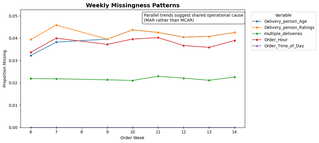

The figure shows that missingness in Delivery_person_Age, Delivery_person_Ratings, multiple_deliveries, and the derived order-time variables follows a similar time pattern across weeks.

Notice that Order_Time_of_Day has identical missingness to Order_Hour, because it is derived from it. This confirms that missingness propagates from the raw timestamp variable.

Two important observations:

Missingness is not constant over time — it fluctuates by week.
The affected variables move together, suggesting a shared underlying process.

If missingness were MCAR (Missing Completely at Random), we would expect no systematic relationship with time or other observable variables. The clear temporal structure makes pure MCAR unlikely.

Instead, the pattern is consistent with a data-generation mechanism linked to onboarding or system changes over time — for example, new delivery drivers entering the platform with partially completed profiles.

This aligns with MAR (Missing At Random): missingness depends on observed variables (such as Order_Week) rather than on the unobserved value itself.

Under MAR, model-based imputation inside a Pipeline is statistically appropriate.

5.7 Build a regression Pipeline

You will now build a `scikit-learn Pipeline to predict Time_taken(min) from operational predictors.

Do not hard-code transformations outside the Pipeline. All preprocessing must live inside it.

Your Pipeline should:

Handle missing values appropriately.
Encode categorical predictors.
Scale numeric predictors.
Be compatible with cross-validation.
Avoid data leakage.

You may consult:

The scikit-learn documentation on Pipelines and ColumnTransformer: https://scikit-learn.org/stable/modules/compose.html
The Orange Juice example at the start of this notebook, where we constructed a full preprocessing + modelling Pipeline.

⚠️ Important

Think carefully about:

Which variables are meaningful predictors.
Which variables are identifiers or raw fields that should not be used.
Whether some variables have no variation in a cross-sectional setting.
Whether engineered variables already replace raw ones.

You are responsible for defining:

numeric_features = [...]
categorical_features = [...]

and constructing an appropriate ColumnTransformer.

❗ Leakage reminder

A Pipeline must be:

Defined before splitting (that’s fine),
But fitted only on training data.

You will later integrate this Pipeline into cross-validation. If preprocessing is done outside the Pipeline, your results are invalid.

Why we use a Pipeline

In scikit-learn, preprocessing and modelling are combined inside a Pipeline.

This ensures that:

Imputation is fitted only on training data,
Scaling uses training statistics,
Categorical encoding is consistent between train and test sets,
No transformation is accidentally applied outside cross-validation.

The Pipeline is the scikit-learn analogue of a recipe + workflow in tidymodels.

✅ One possible solution

# Columns to exclude from modeling
id_cols = [
    "ID", "Delivery_person_ID",
    "Order_Date", "Order_Week",
    "Time_Orderd", "Time_Order_picked",
    "Restaurant_latitude", "Restaurant_longitude",
    "Delivery_location_latitude", "Delivery_location_longitude",
    "Season"  # constant within one week (cross-sectional only)
]

numeric_features = [
    "Delivery_person_Age", "Delivery_person_Ratings",
    "Vehicle_condition", "multiple_deliveries",
    "distance_km", "Order_Hour", "Pickup_Hour"
]

categorical_features = [
    "Weatherconditions", "Road_traffic_density",
    "Type_of_order", "Type_of_vehicle",
    "Festival", "City", "Time_of_Day", "Order_Time_of_Day"
]

numeric_transformer = Pipeline([
    ("imputer", IterativeImputer(
        estimator=RandomForestRegressor(
            n_estimators=50,
            random_state=42,
            n_jobs=-1
        ),
        random_state=42,
        max_iter=10
    )),
    ("scaler", StandardScaler())
])

categorical_transformer = Pipeline([
    ("imputer", SimpleImputer(strategy="most_frequent")),
    ("onehot",  OneHotEncoder(handle_unknown="ignore", sparse_output=False))
])

preprocessor = ColumnTransformer([
    ("num", numeric_transformer, numeric_features),
    ("cat", categorical_transformer, categorical_features)
])
preprocessor.set_output(transform="pandas")

🔍 Pipeline explanation (why each choice was made)

5.7.1 🧭 1. Retain only meaningful operational predictors

Some columns provide context but should not be used as predictors in a cross-sectional model:

Variable(s)	Why not a predictor?
`ID`, `Delivery_person_ID`	Pure identifiers — including them would allow memorisation rather than generalisation.
`Order_Date`, `Order_Week`	Encode calendar position, not operational drivers. Within a single week, `Order_Week` has no variation.
`Time_Orderd`, `Time_Order_picked`	Raw timestamps are granular and cyclical; we replaced them with engineered features (`Order_Hour`, `Pickup_Hour`, `Order_Time_of_Day`).
`Restaurant_`, `Delivery_location_`	Latitude/longitude are difficult for most models to interpret directly. We summarised them into `distance_km`.
`Season`	Constant within the selected week → no signal.

We exclude these columns by simply not passing them to ColumnTransformer. All unlisted columns are dropped automatically.

5.7.2 🌳 2. Tree-based multivariate imputation (IterativeImputer + RandomForest)

We use IterativeImputer with a RandomForestRegressor estimator.

This performs tree-based multivariate imputation:

For a variable with missing values (e.g. Delivery_person_Age),
A random forest is trained using all other predictors,
Missing values are predicted,
The procedure cycles across variables until convergence.

This approach:

Preserves nonlinear relationships
Captures interactions automatically
Avoids distortions introduced by mean/mode imputation
Mirrors bagged-tree imputation in spirit

Crucially, because imputation is inside the Pipeline:

It is fitted only on the training data
The test set is transformed using learned patterns
No leakage occurs

5.7.3 📏 3. StandardScaler: maintain model-agnostic design

After imputation, numeric predictors are standardised (mean = 0, sd = 1).

While tree-based models do not require scaling, including this step ensures the preprocessing remains compatible with scale-sensitive models (e.g., KNN, SVM, penalised regression). This keeps the workflow flexible and reusable.

5.7.4 🧱 4. OneHotEncoder: convert categories into signals

Categorical variables (City, Road_traffic_density, Festival, etc.) are converted into binary indicators.

handle_unknown="ignore" ensures that unseen categories at prediction time do not cause errors.

5.7.5 🔄 5. Why use a Pipeline?

The Pipeline guarantees:

Correct order of transformations
Identical preprocessing for train and test sets
Clean integration with cross-validation
Protection against data leakage

It formalises the contract: raw data → engineered features → imputation → encoding → scaling → model.

5.8 Choose and specify a regression model – LightGBM

We will use LightGBM, a modern gradient-boosted-tree algorithm that is very efficient on large tabular data.

Both LightGBM and XGBoost implement gradient boosting: a sequence of small trees is trained, each correcting residual errors from previous trees. The difference lies in how they grow trees and manage splits:

XGBoost grows trees level-wise (balanced): it splits all leaves at one depth before going deeper. This produces symmetric trees and is often robust on small or moderately sized data.
LightGBM grows trees leaf-wise: it always expands the single leaf that most reduces the loss, yielding deeper, targeted trees. Together with histogram-based binning of features, this makes LightGBM faster and often stronger on large, sparse, or high-cardinality data.

5.8.1 Example specification

lgb_reg = LGBMRegressor(
    n_estimators=500,
    learning_rate=0.1,
    max_depth=6,
    min_child_samples=10,   # slightly larger
    verbose=-1,             # suppress warnings
    random_state=42
)

5.8.2 Common LightGBM tuning parameters

Parameter	What it controls	Intuition
`n_estimators`	total number of trees	more trees can capture more structure but risk overfitting unless `learning_rate` is small
`learning_rate`	step size for each tree’s contribution	small = slower but safer learning; large = faster but riskier
`max_depth`	maximum depth of a single tree	deeper trees capture complex interactions but can overfit
`min_child_samples`	minimum observations in a leaf	prevents tiny leaves that memorize noise
`num_leaves`	number of leaves per tree	key LightGBM parameter; larger = more complex trees
`colsample_bytree`	fraction of predictors sampled at each split	adds randomness, reduces correlation among trees

When might you prefer XGBoost? On smaller datasets, when stability and interpretability matter. When might you prefer LightGBM? For speed on larger tables, many categorical dummies, or limited tuning time.

5.9 Combine preprocessor and model inside a Pipeline

Once your ColumnTransformer preprocessor and model are ready, combine them in a single Pipeline so preprocessing and modeling stay linked. The Pipeline automatically applies preprocessing before fitting or predicting.

reg_pipeline = Pipeline([
    ("preprocessor", preprocessor),
    ("regressor", lgb_reg)
])

5.10 Evaluate the cross-sectional model

Fit your Pipeline on the training set and evaluate predictions on the test set. Use regression metrics such as RMSE, MAE, and R².

🤺 Your turn

Compute and report these metrics for your model. How accurate is the model on unseen data? Does it tend to over- or under-predict delivery time?

✅ One possible solution

target = "Time_taken(min)"
feature_cols = numeric_features + categorical_features

X_cross_train = cross_train[feature_cols]
y_cross_train = cross_train[target]
X_cross_test  = cross_test[feature_cols]
y_cross_test  = cross_test[target]

reg_pipeline.fit(X_cross_train, y_cross_train)
y_pred = reg_pipeline.predict(X_cross_test)

rmse = root_mean_squared_error(y_cross_test, y_pred)
mae  = mean_absolute_error(y_cross_test, y_pred)
r2   = r2_score(y_cross_test, y_pred)
print(f"RMSE: {rmse:.2f}  MAE: {mae:.2f}  R²: {r2:.3f}")

Note

LightGBM may warn that no further splits improve the loss. This simply means a tree cannot be grown further without overfitting. It is not an error.

Output

RMSE: 4.25  MAE: 3.35  R²: 0.789

💬 How to interpret these metrics

These results tell us that our model performs strongly for a single operational week — but with natural real-world limitations.

5.10.1 1️⃣ Accuracy of delivery-time predictions

An RMSE of 4.25 minutes means that, on average, predicted delivery times are within roughly ±4–5 minutes of the true values. Given that most deliveries fall between 10 and 50 minutes, this corresponds to roughly 8–15% of a typical delivery duration — a high level of precision for a real-world logistics process.

The MAE of 3.35 minutes confirms that the typical error is even smaller than the RMSE suggests. The modest gap between RMSE and MAE indicates that large errors exist but are not dominating performance — the model behaves consistently across most deliveries, with only limited extreme deviations.

5.10.2 2️⃣ How much variation the model explains

The R² value of 0.789 means that nearly 79% of all variation in delivery times is explained by the predictors in the model.

This is substantial for operational data driven by human behaviour and environmental conditions. Key contributors likely include:

Distance, capturing spatial effort,
Traffic density, reflecting congestion,
Time-of-day features, capturing demand cycles,
Weather conditions, influencing travel speed.

The remaining ~21% of unexplained variation likely reflects factors not recorded in the dataset, such as:

Restaurant preparation time variability,
Minor route deviations or parking delays,
Driver-specific behaviour,
Localised traffic disruptions.

5.10.3 3️⃣ What this means in practice

For a delivery platform or restaurant manager, this level of accuracy could already be operationally useful:

Estimating realistic customer arrival windows,
Anticipating congestion periods,
Planning driver allocation,
Detecting when deliveries systematically exceed expectations.

5.10.4 4️⃣ Important caveat: one week ≠ generalisability

Because this is a cross-sectional snapshot (one week only), the model has not yet been tested on how relationships evolve over time.

Patterns may shift due to:

Seasonal changes,
New driver onboarding,
Weather transitions,
Changes in traffic patterns.

The next step — time-aware validation — will assess whether this model remains reliable when predicting future weeks rather than just this single operational period.

🤔 Explore residuals: how well does your model really perform?

Numerical metrics tell part of the story — but to see how your model behaves, you need to inspect residuals (the differences between actual and predicted delivery times).

Try plotting:

Predicted vs. actual delivery times → Are most points near the diagonal (perfect predictions)? → Do errors grow with longer delivery times?
Residuals vs. predicted values → Are residuals centered around zero (no systematic bias)? → Do you see patterns that might suggest missing predictors?
Residuals by time of day → Are certain times (e.g., evening rush hours) consistently over- or under-predicted?

Write a short paragraph summarizing what you notice. Does the model perform equally well for all deliveries, or does it struggle under specific conditions?

5.10.5 Cross-validation on the cross-sectional data

So far, you evaluated the model with a single train/test split. In a cross-sectional setting (no time ordering), it is common to use k-fold cross-validation, which splits the training data into k random folds, training on k – 1 folds and validating on the remaining fold in turn. This yields a more robust estimate of performance stability.

🤺 Your turn

Run a 5-fold cross-validation on the cross-sectional training data. Compare the average RMSE and R² to those from the single test-set evaluation. Are they similar? Which estimate do you trust more?

📏 Note on scoring metrics in scikit-learn

In cross_validate(), error-based metrics such as RMSE and MAE are returned as negative values (e.g., neg_root_mean_squared_error).

Why? Because scikit-learn follows a convention where higher scores are always better. Since lower RMSE and MAE are preferable, the library multiplies them by –1 internally so they can be maximized during model selection.

When interpreting results, we therefore multiply these values by –1 again to recover the actual error:

-cv_results["test_neg_root_mean_squared_error"]
-cv_results["test_neg_mean_absolute_error"]

R² does not need this adjustment because higher values are naturally better.

✅ One possible solution

cv_cross = KFold(n_splits=5, shuffle=True, random_state=42)

cv_results = cross_validate(
    reg_pipeline,
    X_cross_train, y_cross_train,
    cv=cv_cross,
    scoring=["neg_root_mean_squared_error", "neg_mean_absolute_error", "r2"],
    return_train_score=False
)

print("RMSE:", round(-cv_results["test_neg_root_mean_squared_error"].mean(), 2))
print("MAE: ", round(-cv_results["test_neg_mean_absolute_error"].mean(), 2))
print("R²:  ", round( cv_results["test_r2"].mean(), 3))

Output

RMSE: 4.36
MAE:  3.42
R²:   0.767

Interpretation:

The cross-validation metrics are slightly weaker than the single test-set evaluation (RMSE 4.36 vs 4.25, R² 0.767 vs 0.789), but remain very close overall.

This small performance drop is expected. Cross-validation repeatedly trains and evaluates the model on different splits of the training data, exposing it to slightly different data structures each time. As a result, CV provides a more conservative and stable estimate of performance.

The consistency between:

Test-set RMSE ≈ 4.25
CV RMSE ≈ 4.36

suggests that the model is not highly sensitive to a particular random split. In other words, performance is reasonably stable across subsamples of the week.

Notice that R² decreased slightly more than RMSE increased. This reflects the fact that R² is sensitive to how well variance is captured across folds, while RMSE reflects absolute prediction error.

When choosing which estimate to trust, cross-validation is generally more reliable because it averages over multiple folds rather than relying on a single train/test division. However, both estimates tell a coherent story: the model explains roughly 75–80% of the variation in delivery time within this operational week.

5.11 Time-aware validation with `TimeSeriesSplit`

In time-dependent data, future information must not influence the model’s training. To mimic real-world deployment, we roll forward through time: train on past weeks, validate on the next week(s).

# Chronological split: 80% train, 20% test
cutoff = int(len(food) * 0.8)
long_train = food.iloc[:cutoff].copy()
long_test  = food.iloc[cutoff:].copy()

cv_long = TimeSeriesSplit(n_splits=6)

⚠️ Avoid leakage!

Never define cross-validation folds on the entire dataset. If you did, the model could “peek” at future data while training, inflating performance. Instead, use only the training portion of your longitudinal split — here called long_train.

5.11.1 How `TimeSeriesSplit` works

TimeSeriesSplit creates a sequence of rolling resamples ordered by row index. Because the data were sorted by Order_Date before splitting, row order corresponds to time order. Each successive fold uses all past rows as training data and the next block of rows as validation — exactly like an expanding window. Unlike KFold, TimeSeriesSplit never shuffles the data and never allows future observations to enter the training set. Each fold expands the training window forward in time.

Peering inside the cross-validation folds

for i, (train_idx, val_idx) in enumerate(cv_long.split(long_train)):
    train_dates = long_train.iloc[train_idx]["Order_Date"]
    val_dates   = long_train.iloc[val_idx]["Order_Date"]
    print(f"Fold {i+1}: train {train_dates.min().date()} → {train_dates.max().date()}"
          f"  |  val {val_dates.min().date()} → {val_dates.max().date()}")

Fold 1: train 2022-02-11 → 2022-02-16  |  val 2022-02-16 → 2022-03-03
Fold 2: train 2022-02-11 → 2022-03-03  |  val 2022-03-03 → 2022-03-08
Fold 3: train 2022-02-11 → 2022-03-08  |  val 2022-03-08 → 2022-03-13
Fold 4: train 2022-02-11 → 2022-03-13  |  val 2022-03-13 → 2022-03-18
Fold 5: train 2022-02-11 → 2022-03-18  |  val 2022-03-18 → 2022-03-24
Fold 6: train 2022-02-11 → 2022-03-24  |  val 2022-03-24 → 2022-03-29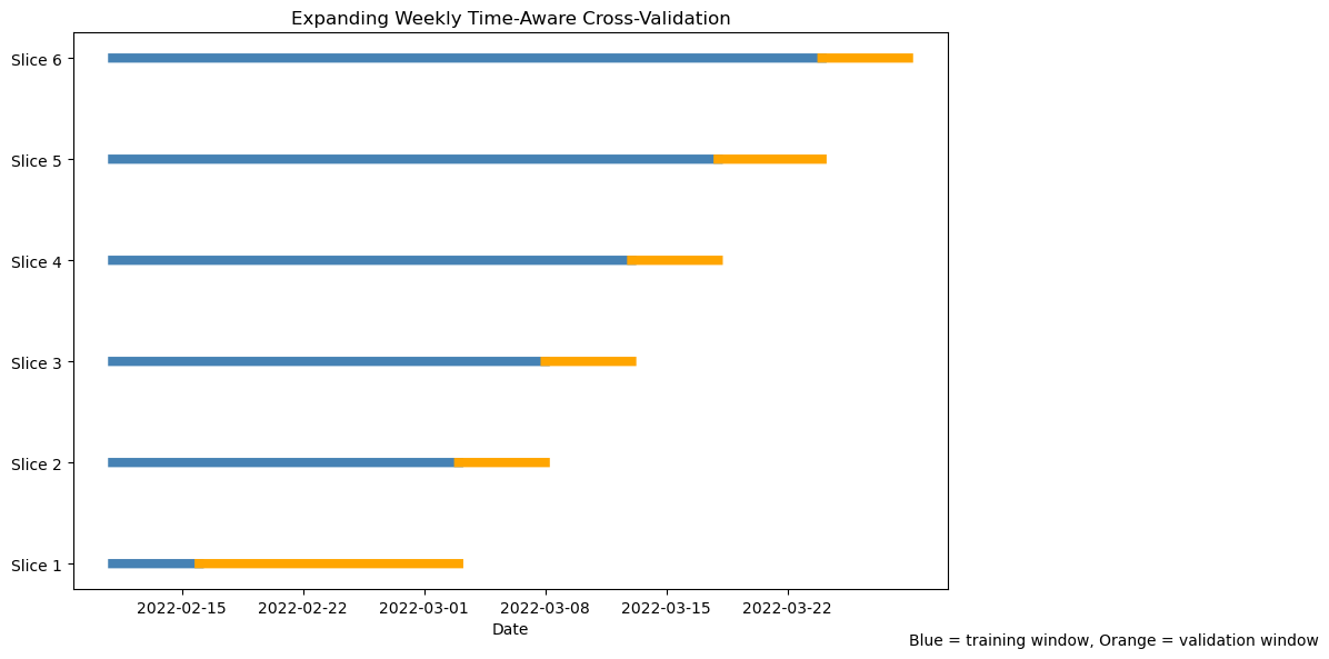

Visualising the folds (code)

# Ensure chronological order
long_train = long_train.sort_values("Order_Date").reset_index(drop=True)

dates = long_train["Order_Date"]

fig, ax = plt.subplots(figsize=(12, 6))

for i, (train_idx, val_idx) in enumerate(cv_long.split(long_train)):

    train_dates = dates.iloc[train_idx]
    val_dates   = dates.iloc[val_idx]

    # Training window
    ax.plot(
        train_dates,
        [i] * len(train_dates),
        color="steelblue",
        linewidth=6
    )

    # Validation window
    ax.plot(
        val_dates,
        [i] * len(val_dates),
        color="orange",
        linewidth=6
    )

ax.set_yticks(range(i + 1))
ax.set_yticklabels([f"Slice {j+1}" for j in range(i + 1)])

ax.set_xlabel("Date")
ax.set_title("Expanding Weekly Time-Aware Cross-Validation")

ax.text(
    dates.iloc[-1],
    -0.8,
    "Blue = training window, Orange = validation window"
)

plt.tight_layout()
plt.show()

5.12 Pipeline and modeling for longitudinal validation

Repeat the full process—Pipeline, model, and evaluation—on the longitudinal setup. Then train and evaluate the model using the time-aware splits created above.

🤺 Your turn

Use cross_validate() with cv=cv_long to fit your LightGBM Pipeline on long_train. Collect metrics (RMSE, MAE, R²) and summarize them.

✅ One possible solution

# For the longitudinal setup, Season is meaningful (training spans multiple seasons)
numeric_features_long = numeric_features  # same as cross-sectional
categorical_features_long = categorical_features + ["Season"]

numeric_transformer_long = Pipeline([
    ("imputer", IterativeImputer(
        estimator=RandomForestRegressor(
            n_estimators=50,
            random_state=42,
            n_jobs=-1
        ),
        random_state=42,
        max_iter=10
    )),
    ("scaler", StandardScaler())
])

categorical_transformer_long = Pipeline([
    ("imputer", SimpleImputer(strategy="most_frequent")),
    # handle_unknown="ignore" handles new categories like "Spring" in test data
    ("onehot",  OneHotEncoder(handle_unknown="ignore", sparse_output=False))
])

preprocessor_long = ColumnTransformer([
    ("num", numeric_transformer_long, numeric_features_long),
    ("cat", categorical_transformer_long, categorical_features_long)
])

long_pipeline = Pipeline([
    ("preprocessor", preprocessor_long),
    ("regressor",    LGBMRegressor(n_estimators=500, learning_rate=0.1,
                                   max_depth=6, random_state=42))
])

X_long_train = long_train[numeric_features_long + categorical_features_long]
y_long_train = long_train[target]

long_cv_results = cross_validate(
    long_pipeline,
    X_long_train, y_long_train,
    cv=cv_long,
    scoring=["neg_root_mean_squared_error", "neg_mean_absolute_error", "r2"],
    return_train_score=False
)

print("RMSE:", round(-long_cv_results["test_neg_root_mean_squared_error"].mean(), 2))
print("MAE: ", round(-long_cv_results["test_neg_mean_absolute_error"].mean(), 2))
print("R²:  ", round( long_cv_results["test_r2"].mean(), 3))

ℹ️ About the LightGBM feature-name warning

You may see warnings stating that feature names are missing. This occurs because ColumnTransformer outputs a NumPy array internally, while LightGBM stores feature names during fitting.

This warning is harmless in our setup and does not affect results.

5.12.1 🧭 Explanation

5.12.1.1 1. `handle_unknown="ignore"` — essential for unseen levels

Because all training data belong to Winter but testing includes Spring deliveries, OneHotEncoder(handle_unknown="ignore") is the scikit-learn equivalent of step_novel() in tidymodels. It gracefully handles new categorical levels at prediction time by encoding them as all-zeros, rather than raising an error.

Without this setting, the Pipeline would fail when encountering "Spring", since the encoder prepared only "Winter" levels. This mimics real-world temporal generalization — when a model trained in one period faces new categories later.

5.12.1.2 2. Normalization kept for generality

Although tree-based models (like LightGBM) don’t require normalized inputs, this normalization step helps if you later try linear, ElasticNet, KNN, or SVM models.

Output

RMSE: 4.06
MAE:  3.21
R²:   0.811

Note: expect slightly different numbers than the cross-sectional test split because (a) folds change over weeks, and (b) training windows grow over time.

💬 Metrics interpretation

The time-aware CV results (RMSE ≈ 4.06, R² ≈ 0.81) are slightly stronger than the cross-sectional CV results.

This suggests that the relationship between predictors and delivery time is relatively stable across adjacent weeks. Because each fold trains on all past data and validates on the next week, the model appears to generalize well over short temporal horizons.

Importantly, this does not mean time validation always improves performance. In many real-world settings, temporal drift weakens predictive power. Here, operational patterns (distance, traffic, weather) seem stable enough that expanding training windows help the model slightly.

5.13 Challenge: comparing designs

Compare your cross-sectional and longitudinal results.

💬 Think about this

Are the results directly comparable? Why or why not?
Which design better represents real-world performance, and why?
How does time-aware validation change your interpretation of model quality?

✅ One possible solution

5.13.1 🔍 Summary of results

Design	RMSE ↓	MAE ↓	R² ↑	Resampling	Notes
Cross-sectional (CV)	4.36	3.42	0.767	Random folds within one week	Stable within a single operational regime
Longitudinal (rolling CV)	4.06	3.21	0.811	Expanding past → future windows	Evaluates temporal generalization

5.13.2 🧭 Interpretation

5.13.2.1 1️⃣ Are the results directly comparable?

Not fully.

The cross-sectional model is evaluated within a single week, using random folds. It measures how well the model captures variation within one operational regime.

The longitudinal model is evaluated across multiple weeks, using expanding windows that respect time order. It measures how well patterns learned from the past transfer to future periods.

Although the same preprocessing and model are used, the two designs answer different questions:

Cross-sectional CV → Can the model explain variation within this week?
Longitudinal CV → Can the model generalize forward in time?

5.13.2.2 2️⃣ Which design better represents real-world deployment?

The time-aware longitudinal design does.

In practice, we train on historical deliveries and predict future ones. We do not randomly mix future observations into training data.

Because TimeSeriesSplit enforces chronological order, it respects temporal causality. This makes it a better approximation of real-world forecasting or operational deployment.

5.13.2.3 3️⃣ Why does the longitudinal model perform slightly better here?

Interestingly, the longitudinal CV metrics are slightly stronger (lower RMSE, higher R²).

This likely reflects two structural differences:

The training window expands over time, giving the model more data.
The data-generating process appears relatively stable across adjacent weeks, so additional history improves estimation rather than introducing drift.

In other contexts with strong seasonal shifts or policy changes, time-aware validation often reduces performance. Here, it instead confirms stability.

5.13.3 🎯 Key takeaway

Cross-sectional validation measures performance within a fixed regime.

Time-aware validation measures performance under temporal evolution.

If a model performs consistently under time-aware validation, it provides stronger evidence that it can be trusted for future predictions — not just for explaining patterns in already-observed data.

For any task involving time, validation design is part of the modeling decision, not an afterthought.

5.14 🧗 Challenge: try another model

Repeat the workflow using a different algorithm of your choice (for example, Elastic-Net, SVM, or KNN). Do not copy specifications here — consult lectures, 📚 labs W02–W05, and the reading week homework for syntax, recommended preprocessing, and tuning guidance.

Evaluate the alternative model on both cross-sectional and time-aware folds and compare results.

💭 Reflection

Which model generalized best over time?
Did any model appear acceptable under random folds but degrade under time-aware validation?
Which preprocessing steps (such as normalization) were essential for your chosen model, and why?
Would your preferred model still perform well if new conditions appeared (e.g., “Summer” deliveries or new cities)?

✅ One possible solution

5.14.1 🔁 Elastic Net regression – cross-sectional design

enet_pipeline = Pipeline([
    ("preprocessor", preprocessor),
    ("regressor", ElasticNet(max_iter=10000, random_state=42))
])

param_grid = {
    "regressor__alpha":   [0.001, 0.01, 0.1, 1.0],
    "regressor__l1_ratio": [0.0, 0.25, 0.5, 0.75, 1.0]
}

enet_search = GridSearchCV(
    enet_pipeline,
    param_grid,
    cv=cv_cross,
    scoring="neg_root_mean_squared_error",
    refit=True,
    n_jobs=-1
)

enet_search.fit(X_cross_train, y_cross_train)

best_enet = enet_search.best_estimator_

# Cross-sectional test performance
y_enet_test = best_enet.predict(X_cross_test)

print("Best params:", enet_search.best_params_)
print("CV RMSE:", round(-enet_search.best_score_, 2))
print("Test RMSE:", round(np.sqrt(mean_squared_error(y_cross_test, y_enet_test)), 2))
print("Test MAE:", round(mean_absolute_error(y_cross_test, y_enet_test), 2))
print("Test R²:", round(r2_score(y_cross_test, y_enet_test), 3))

Output

Best params: {'regressor__alpha': 0.001, 'regressor__l1_ratio': 1.0}
CV RMSE: 6.13
Test RMSE: 6.13
Test MAE: 4.77
Test R²: 0.562

5.14.2 🔁 Elastic Net – longitudinal validation

enet_long_pipeline = Pipeline([
    ("preprocessor", preprocessor_long),
    ("regressor", ElasticNet(max_iter=10000, random_state=42))
])

enet_long_cv = cross_validate(
    enet_long_pipeline,
    X_long_train,
    y_long_train,
    cv=cv_long,
    scoring=["neg_root_mean_squared_error", "neg_mean_absolute_error", "r2"],
    n_jobs=-1
)

print("Long CV RMSE:", round(-enet_long_cv["test_neg_root_mean_squared_error"].mean(), 2))
print("Long CV MAE:", round(-enet_long_cv["test_neg_mean_absolute_error"].mean(), 2))
print("Long CV R²:", round(enet_long_cv["test_r2"].mean(), 3))

Output

Long CV RMSE: 7.45
Long CV MAE: 5.95
Long CV R²: 0.365

5.14.3 📊 Synthesis: comparing LightGBM and ElasticNet

Design	LightGBM RMSE	ElasticNet RMSE	LightGBM R²	ElasticNet R²
Cross-sectional (CV)	4.36	6.13	0.767	—
Test set	4.25	6.13	0.789	0.562
Longitudinal (rolling CV)	4.06	7.45	0.811	0.365

5.14.4 💬 Discussion

Observation	Insight
LightGBM substantially outperforms ElasticNet in all designs	Nonlinear interactions (distance × traffic × weather) matter for delivery time prediction.
ElasticNet performs moderately within one week (R² ≈ 0.56)	Linear structure captures some signal (distance, traffic density), but misses interaction effects.
ElasticNet degrades sharply under time-aware validation (R² drops to 0.37)	Linear relationships do not remain stable across evolving weeks.
LightGBM remains strong under time-aware validation	Boosted trees adapt better to temporal variation and nonlinear structure.

5.14.5 📚 Conceptual takeaway

Lesson	Why it matters
Model flexibility matters when structure is nonlinear	Linear models may underfit complex operational systems.
Temporal validation can change model rankings	A model that looks acceptable under random folds may fail when evaluated chronologically.
Validation design influences interpretation	Cross-sectional CV measures stability within a regime; time-aware CV measures robustness over time.
Interpretability vs. performance trade-off	ElasticNet offers coefficient transparency; LightGBM offers predictive strength.

5.14.6 🎯 Final insight

Under cross-sectional validation, ElasticNet appears serviceable. Under time-aware validation, its performance deteriorates markedly.

This illustrates a critical modeling principle:

Robustness over time is more important than moderate in-sample performance.

For forecasting tasks, validation strategy often reveals more about model reliability than the algorithm choice alone.

6 Classifying deliveries by speed 🚴‍♀️

So far, you have treated delivery time as a continuous variable and built regression models to predict it. We will now reframe the same problem as a classification task: predicting whether a delivery is fast, medium, or slow based on its characteristics.

This shift lets you practice classification workflows and also experiment with techniques for handling class imbalance while keeping the same modelling discipline: time-aware validation, leakage prevention, and Pipelines.

6.1 Define delivery-speed classes

Rather than using arbitrary thresholds (for example “below 30 minutes = fast”), we can define speed relative to distance. A fairer comparison is:

delivery speed = distance / time (km per minute)

food["speed_km_min"] = food["distance_km"] / food["Time_taken(min)"]

q33 = food["speed_km_min"].quantile(0.33)
q67 = food["speed_km_min"].quantile(0.67)

def assign_speed_class(s):
    if s >= q67:
        return "Fast"
    elif s <= q33:
        return "Slow"
    else:
        return "Medium"

food["speed_class"] = food["speed_km_min"].apply(assign_speed_class)

# Ordered categories (nice for display; model treats this as nominal)
food["speed_class"] = pd.Categorical(
    food["speed_class"],
    categories=["Slow", "Medium", "Fast"],
    ordered=True
)

This approach adapts automatically to the dataset’s scale and ensures that roughly one-third of deliveries fall in each class. You can adjust the quantile cut-offs if you wish to make the “Fast” or “Slow” categories narrower.

Alternative definitions

If you prefer a binary classification (for example fast vs not fast), combine “Slow” and “Medium” into a single category. Think about which framing would be more relevant for an operations team (e.g., “will this order likely breach an SLA?”).

6.2 Explore class balance

Before training any classifier, you should always examine how balanced your outcome variable is.

Understanding class proportions helps you decide:

Whether accuracy is meaningful,
Whether macro- or weighted-averaged metrics are appropriate,
Whether class weighting or resampling might be needed.

🤺 Your turn

Compute the count of observations in each speed_class.
Compute the proportion of each class.
Present your results in a clear table.
Briefly comment on whether the dataset appears balanced.

Based on your findings, decide whether macro-averaged metrics are appropriate.

✅ One possible solution

class_balance = (
    food["speed_class"]
    .value_counts()
    .rename("count")
    .to_frame()
    .assign(prop=lambda df: df["count"] / df["count"].sum())
    .sort_index()
)

class_balance

output

        count      prop
Slow    15046  0.330007
Medium  15501  0.339986
Fast    15046  0.330007

In this dataset, the classes are roughly balanced (though Medium is slightly larger). Even in near-balanced settings, we’ll still use macro-averaged metrics so that each class contributes equally.

6.3 🤺 Your turn: build a classification Pipeline

Split the data into training/test sets and create a Pipeline that predicts speed_class from the relevant predictors (distance, traffic, weather, vehicle type, etc.).

Follow the same logic as before but adapt it for classification:

Impute missing numeric values (tree-based imputation is fine, but keep it efficient).
Impute missing categorical values with SimpleImputer(strategy="most_frequent").
One-hot encode categorical variables with OneHotEncoder(handle_unknown="ignore").
Normalize numeric predictors with StandardScaler.
Optionally explore resampling using imblearn only in random CV, not time-aware CV.

Consult the scikit-learn ColumnTransformer documentation for details.

Tip — handling class imbalance with imbalanced-learn (for exploration, not used in the time-aware solution below)

You may see these tools in imbalanced-learn:

from imblearn.pipeline import Pipeline as ImbPipeline
from imblearn.over_sampling import RandomOverSampler
from imblearn.under_sampling import RandomUnderSampler

What they are for:

ImbPipeline allows resampling steps to live inside a Pipeline, so resampling happens correctly within each training fold during cross-validation.
RandomOverSampler duplicates minority-class examples in the training fold.
RandomUnderSampler discards some majority-class examples in the training fold.

Important (design caveat): these assume that rows can be shuffled freely. So they are suitable for random cross-validation (cross-sectional design), but not for time-aware CV such as TimeSeriesSplit.

In this section’s solution, we tune with time-aware CV, so we do not use oversampling/undersampling here. We mention them to guide further exploration later.

⚠️ Important:

Upsampling and downsampling assume that observations can be freely shuffled between resamples. They are suitable for random cross-validation, where all rows are exchangeable. However, they should not be used inside time-aware cross-validation such as TimeSeriesSplit. Doing so would destroy the chronological structure and introduce future information into past folds, leading to data leakage. If you wish to handle imbalance in time-series data, use class-weighting (see this page and this page for more explanations) or use metrics that account for imbalance (macro-F1).

✅ One possible solution

# ----------------------------------------------------------
# Chronological split for classification
# ----------------------------------------------------------
cutoff = int(len(food) * 0.8)
class_train = food.iloc[:cutoff].copy()
class_test  = food.iloc[cutoff:].copy()

class_target = "speed_class"

# ----------------------------------------------------------
# Feature definitions
# (Exclude speed_km_min and Time_taken(min) — they define target)
# ----------------------------------------------------------
numeric_features_class = [
    "Delivery_person_Age", "Delivery_person_Ratings",
    "Vehicle_condition", "multiple_deliveries",
    "distance_km", "Order_Hour", "Pickup_Hour"
]

categorical_features_class = [
    "Weatherconditions", "Road_traffic_density",
    "Type_of_order", "Type_of_vehicle",
    "Festival", "City",
    "Time_of_Day", "Order_Time_of_Day",
    "Season"
]

# ----------------------------------------------------------
# Identify numeric columns that actually have missingness
# ----------------------------------------------------------
numeric_missing = [
    col for col in numeric_features_class
    if class_train[col].isnull().any()
]

numeric_complete = [
    col for col in numeric_features_class
    if col not in numeric_missing
]

# ----------------------------------------------------------
# Leaner tree-based imputation (fast but still nonlinear)
# Apply only to columns that are missing
# ----------------------------------------------------------
rf_imputer = IterativeImputer(
    estimator=RandomForestRegressor(
        n_estimators=20,
        max_depth=5,
        min_samples_leaf=5,
        n_jobs=-1,
        random_state=42
    ),
    max_iter=5,
    random_state=42
)

numeric_pre_impute = ColumnTransformer(
    transformers=[
        ("rf_impute", rf_imputer, numeric_missing),
        ("pass", "passthrough", numeric_complete),
    ],
    remainder="drop",
    verbose_feature_names_out=False
)

numeric_pipeline_cls = Pipeline([
    ("impute_selected", numeric_pre_impute),
    ("scaler", StandardScaler())
])

categorical_transformer_cls = Pipeline([
    ("imputer", SimpleImputer(strategy="most_frequent")),
    ("onehot",  OneHotEncoder(handle_unknown="ignore", sparse_output=False))
])

preprocessor_cls = ColumnTransformer(
    transformers=[
        ("num", numeric_pipeline_cls, numeric_features_class),
        ("cat", categorical_transformer_cls, categorical_features_class),
    ],
    remainder="drop",
    verbose_feature_names_out=False
)

# ----------------------------------------------------------
# Base LightGBM classifier
# We'll tune key parameters with time-aware CV below.
# ----------------------------------------------------------
lgb_base = LGBMClassifier(
    n_estimators=250,
    random_state=42,
    n_jobs=-1,
    verbose=-1
)

class_pipeline = Pipeline([
    ("preprocessor", preprocessor_cls),
    ("classifier", lgb_base)
])

6.4 Choose a classification model

You will now build a classifier to predict speed_class.

You may choose any model covered in lectures (e.g., logistic regression, SVM, KNN, random forest, gradient boosting).

Consult:

Your lecture notes
Labs W02–W05
The Orange Juice example at the beginning of this notebook

Your classifier must:

Be combined with your preprocessing object inside a Pipeline.
Produce class probabilities (required later for ROC AUC and calibration).

🤺 Your turn

Select a classifier.
Combine it with your preprocessing step inside a Pipeline.
Briefly justify your choice of model.

✅ One possible solution

6.4.1 Model choice: LightGBM

We choose LightGBM (gradient boosting) for this task.

Justification in context of this problem:

Delivery speed depends on nonlinear relationships (e.g., distance × traffic × weather).
Interactions between predictors are likely important.
Tree-based boosting models handle nonlinearities and interactions automatically.
LightGBM produces class probabilities (predict_proba), which we require later for ROC AUC and calibration.
It performed strongly in the regression section, giving methodological continuity.

class_pipeline = Pipeline([
    ("preprocessor", preprocessor_cls),
    ("classifier", LGBMClassifier(random_state=42))
])

6.5 Time-aware tuning

Because this is a chronological prediction problem, model validation must respect time ordering.

We therefore tune using time-aware cross-validation.

🤺 Your turn

Use time-aware cross-validation (e.g., TimeSeriesSplit).
Tune your classifier’s hyperparameters.
Use a macro-averaged metric during tuning.
Report the best parameters and the cross-validated performance.

Explain why your chosen metric is appropriate.

✅ One possible solution

cv_class = TimeSeriesSplit(n_splits=6)

X_class_train = class_train[numeric_features_class + categorical_features_class]
y_class_train = class_train[class_target]

param_dist_cls = {
    "classifier__learning_rate":     [0.05, 0.1],
    "classifier__max_depth":         [4, 6],
    "classifier__min_child_samples": [10, 20],
    "classifier__num_leaves":        [15, 31],
}

lgb_tune = RandomizedSearchCV(
    estimator=class_pipeline,
    param_distributions=param_dist_cls,
    n_iter=6,
    cv=cv_class,
    scoring="f1_macro",
    refit=True,
    random_state=42,
    n_jobs=-1
)

lgb_tune.fit(X_class_train, y_class_train)

print("Best params:", lgb_tune.best_params_)
print("Best CV Macro-F1:", round(lgb_tune.best_score_, 3))

Best params: {'classifier__num_leaves': 31, 'classifier__min_child_samples': 10, 'classifier__max_depth': 6, 'classifier__learning_rate': 0.05}
Best CV Macro-F1: 0.863

6.5.1 Why macro-F1 is appropriate here

Macro-F1 gives equal weight to each class:

Slow
Medium
Fast

Even though the dataset is approximately balanced (terciles), the difficulty of predicting each class is not equal.

The Medium class contains borderline deliveries near tercile cut-offs. It is structurally more ambiguous.

If we tuned using accuracy:

The model could perform very well on Slow and Fast
Underperform on Medium
Still look strong overall

Macro-F1 prevents this. It forces the model to perform reasonably well on all classes.

6.6 Evaluate classification performance

Now evaluate the tuned classifier on the held-out test set.

You should report:

The classification report
Multiclass ROC AUC

Then interpret:

Which class is hardest to predict?
Whether errors are symmetric or directional.
Whether the model generalises plausibly forward in time.

🤺 Your turn

Evaluate your tuned classifier on the test set and interpret the results.

✅ One possible solution

X_class_test = class_test[numeric_features_class + categorical_features_class]
y_class_test = class_test[class_target]

best_model = lgb_tune.best_estimator_

y_pred  = best_model.predict(X_class_test)
y_proba = best_model.predict_proba(X_class_test)

print(classification_report(
    y_class_test,
    y_pred,
    target_names=["Slow", "Medium", "Fast"]
))

roc = roc_auc_score(
    y_class_test,
    y_proba,
    multi_class="ovr",
    average="macro"
)

print(f"ROC AUC (macro OvR): {roc:.3f}")

              precision    recall  f1-score   support

        Slow       0.89      0.88      0.88      3182
      Medium       0.79      0.82      0.80      3095
        Fast       0.92      0.90      0.91      2842

    accuracy                           0.86      9119
   macro avg       0.87      0.86      0.87      9119
weighted avg       0.87      0.86      0.86      9119

ROC AUC (macro OvR): 0.971

6.7 Interpretation

6.7.1 1️⃣ Does the model generalise forward in time?

Time-aware CV Macro-F1: 0.863
Test Macro-F1: ≈ 0.87

These are very close.

This small difference indicates:

No meaningful overfitting.
Stable performance when predicting unseen future data.
Forward generalisation is plausible.

Because tuning respected time ordering, this comparison is meaningful.

The absence of a substantial gap between cross-validated and test performance suggests that the model is learning stable operational patterns rather than exploiting week-specific artefacts.

6.7.2 2️⃣ Which class is hardest?

F1-scores:

Fast: 0.91 (reliable for “tight ETA” decisions)
Slow: 0.88 (useful for early warnings / buffer time)
Medium: 0.80

Medium is clearly hardest.

This is expected:

Medium represents borderline deliveries.
It lies between clear extremes.
Ambiguity is built into the target definition.

The model is strongest at detecting clear “Fast” and “Slow” cases.

6.7.3 Confusion matrix

A confusion matrix provides insight into the structure of classification errors.

🤺 Your turn

Plot the confusion matrix and answer:

Which misclassifications are most common?
Are extreme classes confused with each other?
What operational interpretation can you give to the error pattern?
Are all mistakes equally costly in this operational setting?

✅ One possible solution

cm = confusion_matrix(
    y_class_test,
    y_pred,
    labels=["Slow", "Medium", "Fast"]
)

disp = ConfusionMatrixDisplay(
    confusion_matrix=cm,
    display_labels=["Slow", "Medium", "Fast"]
)

disp.plot(cmap="Blues")
plt.title("Confusion Matrix – LightGBM Speed Classifier")
plt.tight_layout()
plt.show()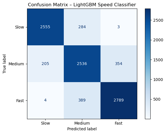

6.7.4 Interpretation of error structure

Most errors involve Medium being confused with either Slow or Fast.
Direct confusion between Slow and Fast is rare.

Operationally:

The model almost never mistakes clearly slow deliveries for clearly fast ones.
Errors cluster around boundary cases.

This is a desirable structure of mistakes.

6.7.5 Calibration of predicted probabilities

High ROC AUC does not guarantee that predicted probabilities are trustworthy.

Calibration checks whether predicted probabilities match observed frequencies.

🤺 Your turn

Plot calibration curves for each class.
Carefully check the internal class order of your classifier before aligning probability columns.
Interpret whether the classifier appears overconfident or underconfident.
If probabilities were miscalibrated, how might that affect decision thresholds?

✅ One possible solution

cls_order = list(best_model.named_steps["classifier"].classes_)
proba_col = {label: i for i, label in enumerate(cls_order)}

fig, axes = plt.subplots(1, 3, figsize=(15, 4))
labels_to_plot = ["Slow", "Medium", "Fast"]

for j, label in enumerate(labels_to_plot):
    i = proba_col[label]

    prob_true, prob_pred = calibration_curve(
        (y_class_test == label).astype(int),
        y_proba[:, i],
        n_bins=10,
        strategy="quantile"
    )

    axes[j].plot(prob_pred, prob_true, marker="o")
    axes[j].plot([0, 1], [0, 1], linestyle="--")
    axes[j].set_title(f"Calibration: {label}")
    axes[j].set_xlabel("Predicted probability")
    axes[j].set_ylabel("Observed frequency")

plt.tight_layout()
plt.show()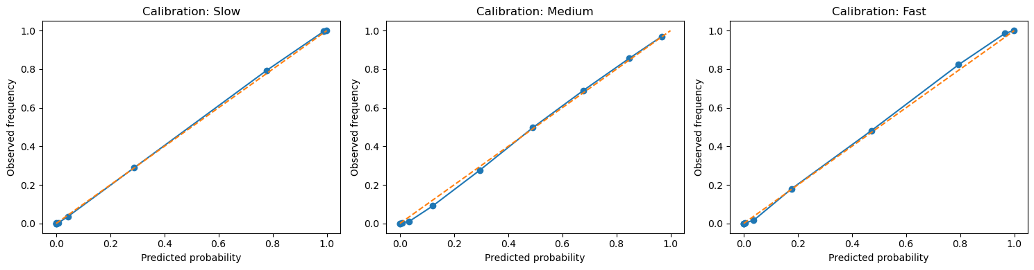

6.7.6 Calibration interpretation

All curves closely follow the diagonal.

This means:

The model’s probability estimates are well aligned with reality.
If it predicts 80% probability for “Fast”, the event occurs roughly 80% of the time.
The model is both discriminative and well calibrated.

🧠 Should the classifier be recalibrated?

scikit-learn provides CalibratedClassifierCV for probability recalibration (Platt scaling or isotonic regression).

Documentation:
https://scikit-learn.org/stable/modules/calibration.html

Recalibration can improve probability estimates when a classifier is systematically overconfident or underconfident.

However, two important considerations apply here:

Chronology must still be respected.
In a time-aware setting, recalibration must use only past data to adjust probabilities for future data.
Random folds are not appropriate.
Using default cross-validation inside CalibratedClassifierCV would violate temporal ordering.

To recalibrate properly in this context, calibration would need to be performed inside a time-aware validation structure (e.g., nested TimeSeriesSplit).

In the current results, the calibration curves already follow the diagonal closely. There is no systematic deviation suggesting overconfidence or underconfidence.

Therefore, recalibration is unnecessary here.

Calibration should be introduced only when diagnostics indicate a clear probability distortion.

Cost asymmetry and modelling decisions

Up to this point, the modelling workflow has focused on:

Balanced evaluation (macro-F1),
Time-aware validation,
Forward generalisation,
Calibration of predicted probabilities.

All of these concern statistical performance.

However, deployment introduces a different type of question:

Are all classification errors equally costly in practice?

In food delivery, they are unlikely to be.

Consider two mistakes:

Predicting “Fast” when the delivery is actually “Slow”. This may lead to unrealistic customer expectations, negative reviews, and reputational damage.
Predicting “Slow” when the delivery is actually “Fast”. This may result in conservative estimates but rarely causes dissatisfaction.

These two errors are not symmetric in their operational consequences.

This is called cost asymmetry.

6.8 Cost asymmetry versus class imbalance

It is important to distinguish two separate ideas.

6.8.1 Class imbalance

Class imbalance refers to unequal frequencies in the dataset.

For example:

70% of observations belong to one class.
15% belong to each of the others.

This is a statistical property of the data distribution.

In this dataset, the classes were constructed using terciles, so they are roughly balanced in frequency.

6.8.2 Cost asymmetry

Cost asymmetry refers to unequal consequences of mistakes.

Even when classes are perfectly balanced in frequency, the impact of different errors may not be equal.

Class imbalance is about how often events occur. Cost asymmetry is about how costly different mistakes are.

These are conceptually independent.

6.9 The modelling pipeline has different layers

There are several distinct stages in the modelling process. Each stage answers a different question.

Understanding this separation avoids confusion.

6.9.1 1️⃣ Evaluation metric — how performance is measured

The choice of macro-F1 affects how performance is summarised during tuning.

Macro-F1:

Computes F1-score separately for each class.
Averages them equally.

It does not change the model. It changes how model quality is evaluated.

Choosing macro-F1 expresses the following preference:

Performance should be balanced across all classes.

This is an evaluation-level decision.

6.9.2 2️⃣ Training objective — how the model learns

During training, the model minimises a loss function.

Class weights modify this loss function.

For example:

LGBMClassifier(
    class_weight={
        "Slow": 1.5,
        "Medium": 1.0,
        "Fast": 1.0
    }
)

This increases the penalty for misclassifying Slow.

The optimisation process will therefore prioritise reducing errors on Slow.

Class weights:

Do not change the evaluation metric.
Do not change the decision rule.
Only change how the model parameters are learned.

This is a training-level modification.

6.9.3 3️⃣ Decision rule — how probabilities become labels

After training, the classifier outputs probabilities.

By default, the predicted class is the one with the highest probability.

However, that rule can be adjusted.

For example, require higher confidence before predicting Fast:

fast_idx = proba_col["Fast"]

custom_pred = np.where(
    y_proba[:, fast_idx] > 0.85,
    "Fast",
    y_pred
)

This does not retrain the model.

It changes how predicted probabilities are translated into decisions.

This is a decision-level modification.

When asymmetric decision thresholds are introduced (e.g., requiring high confidence before predicting Fast), calibration becomes even more important. Poorly calibrated probabilities can distort cost-sensitive decision rules.

6.10 Where cost-sensitive learning fits

Cost-sensitive learning is not a single technique.

It is a modelling approach in which the objective explicitly reflects unequal error costs.

There are different ways to incorporate cost asymmetry:

Modifying the loss function (e.g., via class weights),
Designing a custom cost matrix,
Adjusting decision thresholds,
Combining training and decision adjustments.

In other words:

Cost-sensitive modelling is a framework in which the model is deliberately adjusted to reflect unequal consequences of errors.

Class weights and threshold tuning are implementation mechanisms that can be used within that framework. Importantly, if cost-sensitive adjustments are introduced, they must still respect the chronological validation design used earlier. Any modification to the training objective or decision rule must be evaluated using time-aware cross-validation, not random folds.

They operate at different stages of the modelling pipeline and influence different aspects of behaviour. Confusing them can lead to incorrect assumptions about how and where modelling choices take effect.

6.11 Why this distinction matters here

The current classifier:

Is statistically strong (Macro-F1 ≈ 0.87),
Generalises forward in time (CV ≈ 0.863 vs test ≈ 0.87),
Shows structured and interpretable error patterns,
Produces well-calibrated probabilities.

Whether to introduce class weighting or threshold adjustments depends on operational priorities.

If late deliveries become especially costly, the modelling objective may change.

That is not a statistical necessity.

It is a business decision.

Some practice

To observe the practical effect of cost-sensitive adjustments:

Refit the model with class weights applied during training.
Compare recall and precision for Slow and Fast.
Compare to the model without class weights and check whether metrics improve or whether trade-offs emerge.

Cost-sensitive adjustments often improve one metric at the expense of another. Observing these trade-offs makes the concept concrete.

6.12 Exploring imbalance strategies

Even if the dataset appears balanced, use this as a controlled experiment.

🤺 Your turn

Using the cross-sectional random CV design (not time-aware CV):

Try oversampling and/or undersampling.
Compare recall for the hardest class.
Explain why these methods are not appropriate inside time-aware validation.

Reminder

Oversampling/undersampling are mentioned to guide exploration — they are not appropriate inside TimeSeriesSplit because they would invalidate temporal ordering.

7 To read further about `Pipelines`

To read further about Pipelines’s functionalities, you could have a look at:

this Medium post
this tutorial on Python-Bloggers
or look at the Pipeline documentation and examples that come with it.

	steps steps: list of tuples List of (name of step, estimator) tuples that are to be chained in sequential order. To be compatible with the scikit-learn API, all steps must define `fit`. All non-last steps must also define `transform`. See :ref:`Combining Estimators ` for more details.	[('preprocessor', ...), ('classifier', ...)]
	transform_input transform_input: list of str, default=None The names of the :term:`metadata` parameters that should be transformed by the pipeline before passing it to the step consuming it. This enables transforming some input arguments to ``fit`` (other than ``X``) to be transformed by the steps of the pipeline up to the step which requires them. Requirement is defined via :ref:`metadata routing `. For instance, this can be used to pass a validation set through the pipeline. You can only set this if metadata routing is enabled, which you can enable using ``sklearn.set_config(enable_metadata_routing=True)``. .. versionadded:: 1.6	None
	memory memory: str or object with the joblib.Memory interface, default=None Used to cache the fitted transformers of the pipeline. The last step will never be cached, even if it is a transformer. By default, no caching is performed. If a string is given, it is the path to the caching directory. Enabling caching triggers a clone of the transformers before fitting. Therefore, the transformer instance given to the pipeline cannot be inspected directly. Use the attribute ``named_steps`` or ``steps`` to inspect estimators within the pipeline. Caching the transformers is advantageous when fitting is time consuming. See :ref:`sphx_glr_auto_examples_neighbors_plot_caching_nearest_neighbors.py` for an example on how to enable caching.	None
	verbose verbose: bool, default=False If True, the time elapsed while fitting each step will be printed as it is completed.	False

	transformers transformers: list of tuples List of (name, transformer, columns) tuples specifying the transformer objects to be applied to subsets of the data. name : str Like in Pipeline and FeatureUnion, this allows the transformer and its parameters to be set using ``set_params`` and searched in grid search. transformer : {'drop', 'passthrough'} or estimator Estimator must support :term:`fit` and :term:`transform`. Special-cased strings 'drop' and 'passthrough' are accepted as well, to indicate to drop the columns or to pass them through untransformed, respectively. columns : str, array-like of str, int, array-like of int, array-like of bool, slice or callable Indexes the data on its second axis. Integers are interpreted as positional columns, while strings can reference DataFrame columns by name. A scalar string or int should be used where ``transformer`` expects X to be a 1d array-like (vector), otherwise a 2d array will be passed to the transformer. A callable is passed the input data `X` and can return any of the above. To select multiple columns by name or dtype, you can use :obj:`make_column_selector`.	[('num', ...), ('cat', ...)]
	remainder remainder: {'drop', 'passthrough'} or estimator, default='drop' By default, only the specified columns in `transformers` are transformed and combined in the output, and the non-specified columns are dropped. (default of ``'drop'``). By specifying ``remainder='passthrough'``, all remaining columns that were not specified in `transformers`, but present in the data passed to `fit` will be automatically passed through. This subset of columns is concatenated with the output of the transformers. For dataframes, extra columns not seen during `fit` will be excluded from the output of `transform`. By setting ``remainder`` to be an estimator, the remaining non-specified columns will use the ``remainder`` estimator. The estimator must support :term:`fit` and :term:`transform`. Note that using this feature requires that the DataFrame columns input at :term:`fit` and :term:`transform` have identical order.	'drop'
	sparse_threshold sparse_threshold: float, default=0.3 If the output of the different transformers contains sparse matrices, these will be stacked as a sparse matrix if the overall density is lower than this value. Use ``sparse_threshold=0`` to always return dense. When the transformed output consists of all dense data, the stacked result will be dense, and this keyword will be ignored.	0.3
	n_jobs n_jobs: int, default=None Number of jobs to run in parallel. ``None`` means 1 unless in a :obj:`joblib.parallel_backend` context. ``-1`` means using all processors. See :term:`Glossary ` for more details.	None
	transformer_weights transformer_weights: dict, default=None Multiplicative weights for features per transformer. The output of the transformer is multiplied by these weights. Keys are transformer names, values the weights.	None
	verbose verbose: bool, default=False If True, the time elapsed while fitting each transformer will be printed as it is completed.	False
	verbose_feature_names_out verbose_feature_names_out: bool, str or Callable[[str, str], str], default=True - If True, :meth:`ColumnTransformer.get_feature_names_out` will prefix all feature names with the name of the transformer that generated that feature. It is equivalent to setting `verbose_feature_names_out="{transformer_name}__{feature_name}"`. - If False, :meth:`ColumnTransformer.get_feature_names_out` will not prefix any feature names and will error if feature names are not unique. - If ``Callable[[str, str], str]``, :meth:`ColumnTransformer.get_feature_names_out` will rename all the features using the name of the transformer. The first argument of the callable is the transformer name and the second argument is the feature name. The returned string will be the new feature name. - If ``str``, it must be a string ready for formatting. The given string will be formatted using two field names: ``transformer_name`` and ``feature_name``. e.g. ``"{feature_name}__{transformer_name}"``. See :meth:`str.format` method from the standard library for more info. .. versionadded:: 1.0 .. versionchanged:: 1.6 `verbose_feature_names_out` can be a callable or a string to be formatted.	True
	force_int_remainder_cols force_int_remainder_cols: bool, default=False This parameter has no effect. .. note:: If you do not access the list of columns for the remainder columns in the `transformers_` fitted attribute, you do not need to set this parameter. .. versionadded:: 1.5 .. versionchanged:: 1.7 The default value for `force_int_remainder_cols` will change from `True` to `False` in version 1.7. .. deprecated:: 1.7 `force_int_remainder_cols` is deprecated and will be removed in 1.9.	'deprecated'

	categories categories: 'auto' or a list of array-like, default='auto' Categories (unique values) per feature: - 'auto' : Determine categories automatically from the training data. - list : ``categories[i]`` holds the categories expected in the ith column. The passed categories should not mix strings and numeric values within a single feature, and should be sorted in case of numeric values. The used categories can be found in the ``categories_`` attribute. .. versionadded:: 0.20	'auto'
	drop drop: {'first', 'if_binary'} or an array-like of shape (n_features,), default=None Specifies a methodology to use to drop one of the categories per feature. This is useful in situations where perfectly collinear features cause problems, such as when feeding the resulting data into an unregularized linear regression model. However, dropping one category breaks the symmetry of the original representation and can therefore induce a bias in downstream models, for instance for penalized linear classification or regression models. - None : retain all features (the default). - 'first' : drop the first category in each feature. If only one category is present, the feature will be dropped entirely. - 'if_binary' : drop the first category in each feature with two categories. Features with 1 or more than 2 categories are left intact. - array : ``drop[i]`` is the category in feature ``X[:, i]`` that should be dropped. When `max_categories` or `min_frequency` is configured to group infrequent categories, the dropping behavior is handled after the grouping. .. versionadded:: 0.21 The parameter `drop` was added in 0.21. .. versionchanged:: 0.23 The option `drop='if_binary'` was added in 0.23. .. versionchanged:: 1.1 Support for dropping infrequent categories.	'first'
	sparse_output sparse_output: bool, default=True When ``True``, it returns a :class:`scipy.sparse.csr_matrix`, i.e. a sparse matrix in "Compressed Sparse Row" (CSR) format. .. versionadded:: 1.2 `sparse` was renamed to `sparse_output`	False
	dtype dtype: number type, default=np.float64 Desired dtype of output.	<class 'numpy.float64'>
	handle_unknown handle_unknown: {'error', 'ignore', 'infrequent_if_exist', 'warn'}, default='error' Specifies the way unknown categories are handled during :meth:`transform`. - 'error' : Raise an error if an unknown category is present during transform. - 'ignore' : When an unknown category is encountered during transform, the resulting one-hot encoded columns for this feature will be all zeros. In the inverse transform, an unknown category will be denoted as None. - 'infrequent_if_exist' : When an unknown category is encountered during transform, the resulting one-hot encoded columns for this feature will map to the infrequent category if it exists. The infrequent category will be mapped to the last position in the encoding. During inverse transform, an unknown category will be mapped to the category denoted `'infrequent'` if it exists. If the `'infrequent'` category does not exist, then :meth:`transform` and :meth:`inverse_transform` will handle an unknown category as with `handle_unknown='ignore'`. Infrequent categories exist based on `min_frequency` and `max_categories`. Read more in the :ref:`User Guide `. - 'warn' : When an unknown category is encountered during transform a warning is issued, and the encoding then proceeds as described for `handle_unknown="infrequent_if_exist"`. .. versionchanged:: 1.1 `'infrequent_if_exist'` was added to automatically handle unknown categories and infrequent categories. .. versionadded:: 1.6 The option `"warn"` was added in 1.6.	'ignore'
	min_frequency min_frequency: int or float, default=None Specifies the minimum frequency below which a category will be considered infrequent. - If `int`, categories with a smaller cardinality will be considered infrequent. - If `float`, categories with a smaller cardinality than `min_frequency * n_samples` will be considered infrequent. .. versionadded:: 1.1 Read more in the :ref:`User Guide `.	None
	max_categories max_categories: int, default=None Specifies an upper limit to the number of output features for each input feature when considering infrequent categories. If there are infrequent categories, `max_categories` includes the category representing the infrequent categories along with the frequent categories. If `None`, there is no limit to the number of output features. .. versionadded:: 1.1 Read more in the :ref:`User Guide `.	None
	feature_name_combiner feature_name_combiner: "concat" or callable, default="concat" Callable with signature `def callable(input_feature, category)` that returns a string. This is used to create feature names to be returned by :meth:`get_feature_names_out`. `"concat"` concatenates encoded feature name and category with `feature + "_" + str(category)`.E.g. feature X with values 1, 6, 7 create feature names `X_1, X_6, X_7`. .. versionadded:: 1.3	'concat'

	penalty penalty: {'l1', 'l2', 'elasticnet', None}, default='l2' Specify the norm of the penalty: - `None`: no penalty is added; - `'l2'`: add a L2 penalty term and it is the default choice; - `'l1'`: add a L1 penalty term; - `'elasticnet'`: both L1 and L2 penalty terms are added. .. warning:: Some penalties may not work with some solvers. See the parameter `solver` below, to know the compatibility between the penalty and solver. .. versionadded:: 0.19 l1 penalty with SAGA solver (allowing 'multinomial' + L1) .. deprecated:: 1.8 `penalty` was deprecated in version 1.8 and will be removed in 1.10. Use `l1_ratio` instead. `l1_ratio=0` for `penalty='l2'`, `l1_ratio=1` for `penalty='l1'` and `l1_ratio` set to any float between 0 and 1 for `'penalty='elasticnet'`.	'deprecated'
	C C: float, default=1.0 Inverse of regularization strength; must be a positive float. Like in support vector machines, smaller values specify stronger regularization. `C=np.inf` results in unpenalized logistic regression. For a visual example on the effect of tuning the `C` parameter with an L1 penalty, see: :ref:`sphx_glr_auto_examples_linear_model_plot_logistic_path.py`.	1.0
	l1_ratio l1_ratio: float, default=0.0 The Elastic-Net mixing parameter, with `0 <= l1_ratio <= 1`. Setting `l1_ratio=1` gives a pure L1-penalty, setting `l1_ratio=0` a pure L2-penalty. Any value between 0 and 1 gives an Elastic-Net penalty of the form `l1_ratio * L1 + (1 - l1_ratio) * L2`. .. warning:: Certain values of `l1_ratio`, i.e. some penalties, may not work with some solvers. See the parameter `solver` below, to know the compatibility between the penalty and solver. .. versionchanged:: 1.8 Default value changed from None to 0.0. .. deprecated:: 1.8 `None` is deprecated and will be removed in version 1.10. Always use `l1_ratio` to specify the penalty type.	0.0
	dual dual: bool, default=False Dual (constrained) or primal (regularized, see also :ref:`this equation `) formulation. Dual formulation is only implemented for l2 penalty with liblinear solver. Prefer `dual=False` when n_samples > n_features.	False
	tol tol: float, default=1e-4 Tolerance for stopping criteria.	0.0001
	fit_intercept fit_intercept: bool, default=True Specifies if a constant (a.k.a. bias or intercept) should be added to the decision function.	True
	intercept_scaling intercept_scaling: float, default=1 Useful only when the solver `liblinear` is used and `self.fit_intercept` is set to `True`. In this case, `x` becomes `[x, self.intercept_scaling]`, i.e. a "synthetic" feature with constant value equal to `intercept_scaling` is appended to the instance vector. The intercept becomes ``intercept_scaling * synthetic_feature_weight``. .. note:: The synthetic feature weight is subject to L1 or L2 regularization as all other features. To lessen the effect of regularization on synthetic feature weight (and therefore on the intercept) `intercept_scaling` has to be increased.	1
	class_weight class_weight: dict or 'balanced', default=None Weights associated with classes in the form ``{class_label: weight}``. If not given, all classes are supposed to have weight one. The "balanced" mode uses the values of y to automatically adjust weights inversely proportional to class frequencies in the input data as ``n_samples / (n_classes * np.bincount(y))``. Note that these weights will be multiplied with sample_weight (passed through the fit method) if sample_weight is specified. .. versionadded:: 0.17 class_weight='balanced'	None
	random_state random_state: int, RandomState instance, default=None Used when ``solver`` == 'sag', 'saga' or 'liblinear' to shuffle the data. See :term:`Glossary ` for details.	42
	solver solver: {'lbfgs', 'liblinear', 'newton-cg', 'newton-cholesky', 'sag', 'saga'}, default='lbfgs' Algorithm to use in the optimization problem. Default is 'lbfgs'. To choose a solver, you might want to consider the following aspects: - 'lbfgs' is a good default solver because it works reasonably well for a wide class of problems. - For :term:`multiclass` problems (`n_classes >= 3`), all solvers except 'liblinear' minimize the full multinomial loss, 'liblinear' will raise an error. - 'newton-cholesky' is a good choice for `n_samples` >> `n_features * n_classes`, especially with one-hot encoded categorical features with rare categories. Be aware that the memory usage of this solver has a quadratic dependency on `n_features * n_classes` because it explicitly computes the full Hessian matrix. - For small datasets, 'liblinear' is a good choice, whereas 'sag' and 'saga' are faster for large ones; - 'liblinear' can only handle binary classification by default. To apply a one-versus-rest scheme for the multiclass setting one can wrap it with the :class:`~sklearn.multiclass.OneVsRestClassifier`. .. warning:: The choice of the algorithm depends on the penalty chosen (`l1_ratio=0` for L2-penalty, `l1_ratio=1` for L1-penalty and `0 < l1_ratio < 1` for Elastic-Net) and on (multinomial) multiclass support: ================= ======================== ====================== solver l1_ratio multinomial multiclass ================= ======================== ====================== 'lbfgs' l1_ratio=0 yes 'liblinear' l1_ratio=1 or l1_ratio=0 no 'newton-cg' l1_ratio=0 yes 'newton-cholesky' l1_ratio=0 yes 'sag' l1_ratio=0 yes 'saga' 0<=l1_ratio<=1 yes ================= ======================== ====================== .. note:: 'sag' and 'saga' fast convergence is only guaranteed on features with approximately the same scale. You can preprocess the data with a scaler from :mod:`sklearn.preprocessing`. .. seealso:: Refer to the :ref:`User Guide ` for more information regarding :class:`LogisticRegression` and more specifically the :ref:`Table ` summarizing solver/penalty supports. .. versionadded:: 0.17 Stochastic Average Gradient (SAG) descent solver. Multinomial support in version 0.18. .. versionadded:: 0.19 SAGA solver. .. versionchanged:: 0.22 The default solver changed from 'liblinear' to 'lbfgs' in 0.22. .. versionadded:: 1.2 newton-cholesky solver. Multinomial support in version 1.6.	'lbfgs'
	max_iter max_iter: int, default=100 Maximum number of iterations taken for the solvers to converge.	1000
	verbose verbose: int, default=0 For the liblinear and lbfgs solvers set verbose to any positive number for verbosity.	0
	warm_start warm_start: bool, default=False When set to True, reuse the solution of the previous call to fit as initialization, otherwise, just erase the previous solution. Useless for liblinear solver. See :term:`the Glossary `. .. versionadded:: 0.17 warm_start to support lbfgs, newton-cg, sag, saga solvers.	False
	n_jobs n_jobs: int, default=None Does not have any effect. .. deprecated:: 1.8 `n_jobs` is deprecated in version 1.8 and will be removed in 1.10.	None

1 Introduction

2 🎯 Learning objectives

3 ⚙️ Set-up

3.1 Download dataset and solution notebook

3.2 Install needed libraries (if not done already)

3.3 Import needed libraries

4 🍊 Orange-juice warm-up

4.1 Load and explore the data

4.2 Sampling and stratified splitting

4.3 Feature engineering: add a season variable

4.4 Understanding Pipeline

4.4.1 Step 1 — Separate variables by type

4.4.2 Step 2 — Define transformations for each type

4.4.2.1 Numeric variables

4.4.2.2 Categorical variables

4.4.3 Step 3 — Combine transformations with ColumnTransformer

4.4.4 Step 4 — Build the full modelling pipeline

4.5 Why is this better than doing it step-by-step?

4.5.1 Conceptual Summary

4.5.2 StandardScaler

4.5.2.1 Why standardise?

4.6 Choose a model

4.7 Build and fit the Pipeline

4.8 Fit and evaluate the model

4.8.1 How fit() and predict() work

4.8.2 Choosing appropriate metrics

5 Food delivery dataset 🛵

5.1 Load and explore the data

5.1.0.1 Why dayfirst=True?

5.1.0.2 Why group by week rather than day or month?

5.2 Create a seasonal feature

5.3 Compute a simple distance feature

5.4 Create time-of-day features

5.4.1 🌆 Why this matters

5.5 Create a cross-sectional dataset and training/test split

5.6 Handle missing data with iterative imputation

5.6.1 What is iterative imputation?

5.7 Build a regression Pipeline

5.7.1 🧭 1. Retain only meaningful operational predictors

5.7.2 🌳 2. Tree-based multivariate imputation (IterativeImputer + RandomForest)

5.7.3 📏 3. StandardScaler: maintain model-agnostic design

5.7.4 🧱 4. OneHotEncoder: convert categories into signals

5.7.5 🔄 5. Why use a Pipeline?

5.8 Choose and specify a regression model – LightGBM

5.8.1 Example specification

5.8.2 Common LightGBM tuning parameters

5.9 Combine preprocessor and model inside a Pipeline

5.10 Evaluate the cross-sectional model

5.10.1 1️⃣ Accuracy of delivery-time predictions

5.10.2 2️⃣ How much variation the model explains

5.10.3 3️⃣ What this means in practice

5.10.4 4️⃣ Important caveat: one week ≠ generalisability

5.10.5 Cross-validation on the cross-sectional data

5.11 Time-aware validation with TimeSeriesSplit

5.11.1 How TimeSeriesSplit works

5.12 Pipeline and modeling for longitudinal validation

5.12.1 🧭 Explanation

5.12.1.1 1. handle_unknown="ignore" — essential for unseen levels

5.12.1.2 2. Normalization kept for generality

5.13 Challenge: comparing designs

5.13.1 🔍 Summary of results

5.13.2 🧭 Interpretation

5.13.2.1 1️⃣ Are the results directly comparable?

5.13.2.2 2️⃣ Which design better represents real-world deployment?

5.13.2.3 3️⃣ Why does the longitudinal model perform slightly better here?

5.13.3 🎯 Key takeaway

5.14 🧗 Challenge: try another model

5.14.1 🔁 Elastic Net regression – cross-sectional design

5.14.2 🔁 Elastic Net – longitudinal validation

5.14.3 📊 Synthesis: comparing LightGBM and ElasticNet

5.14.4 💬 Discussion

5.14.5 📚 Conceptual takeaway

5.14.6 🎯 Final insight

6 Classifying deliveries by speed 🚴‍♀️

6.1 Define delivery-speed classes

6.2 Explore class balance

6.3 🤺 Your turn: build a classification Pipeline

6.4 Choose a classification model

6.4.1 Model choice: LightGBM

6.5 Time-aware tuning

4.4 Understanding `Pipeline`

4.4.3 Step 3 — Combine transformations with `ColumnTransformer`

4.8.1 How `fit()` and `predict()` work

5.1.0.1 Why `dayfirst=True`?

5.11 Time-aware validation with `TimeSeriesSplit`

5.11.1 How `TimeSeriesSplit` works

5.12.1.1 1. `handle_unknown="ignore"` — essential for unseen levels

7 To read further about `Pipelines`