✅ A Possible Model Solution for the W08 Summative

Author

Dr Ghita Berrada

Warning

What follows is a possible solution for the W08 summative. Note that I purposely avoided very elaborate solutions here and avoided optimizing the performance of the models to death. I tried to go for rather straightforward but justified solutions.

⚙️ Setup

import pandas as pd
import numpy as np
import missingno as msno
import matplotlib.pyplot as plt
import matplotlib.ticker as mticker
import plotly.express as px
from plotly.subplots import make_subplots
import plotly.graph_objects as go
import seaborn as sns
from statsmodels.stats.outliers_influence import variance_inflation_factor
from sklearn.linear_model import LinearRegression, LogisticRegression
from sklearn.preprocessing import StandardScaler
from sklearn.model_selection import TimeSeriesSplit, RandomizedSearchCV,cross_validate, GridSearchCV
from sklearn.pipeline import Pipeline
from sklearn.feature_selection import SequentialFeatureSelector
from sklearn.metrics import (
    r2_score, mean_absolute_error, mean_squared_error,
    f1_score, precision_score, recall_score,
    roc_auc_score, average_precision_score,
    balanced_accuracy_score, roc_curve,
    precision_recall_curve, confusion_matrix
)
from imblearn.ensemble import BalancedRandomForestClassifier
import shap
# Importing LightGBM
import lightgbm as lgb

import warnings
warnings.filterwarnings('ignore')

plt.style.use('seaborn-v0_8-whitegrid')

Part 1: predicting next-month gold returns

1.3 Construction and finalisation of the dataset

1.3.1 Constructing the target variable

We begin by loading the main monthly dataset and constructing the monthly gold return series.

gold = pd.read_csv('data/gold_price_prediction_dataset.csv', parse_dates=['date'])
gold = gold.sort_values('date').reset_index(drop=True)

# Compute monthly percentage return: r_t = 100 * (P_t - P_{t-1}) / P_{t-1}
gold['gold_return'] = 100 * gold['gold_price'].pct_change()

# The TARGET is next-month return: r_{t+1}
# Shift gold_return back by one row so that row t holds the return realised at t+1
gold['target'] = gold['gold_return'].shift(-1)

Why this alignment?

Each row of our modelling dataset represents month $t$. The predictors observed in month $t$ should be paired with the outcome observed in month $t+1$ i.e the return that a trader, having seen this month’s data, would be trying to predict. Pairing predictors with the contemporaneous return would be a data leakage error: in a real forecasting setting, the return for month $t$ is only realised at the end of month $t$, after the predictor data has been observed. This is one of the most common errors in financial forecasting exercises and must be verified explicitly.

Verification:

jan20 = gold[gold['date'] == '2020-01-01'].iloc[0]
feb20 = gold[gold['date'] == '2020-02-01'].iloc[0]
computed_return = 100 * (feb20['gold_price'] - jan20['gold_price']) / jan20['gold_price']
print(f"Jan 2020 gold price: {jan20['gold_price']:.2f}")
print(f"Feb 2020 gold price: {feb20['gold_price']:.2f}")
print(f"Computed Feb 2020 return: {computed_return:.4f}")
print(f"Value of 'target' in Jan 2020 row: {jan20['target']:.4f}")

Jan 2020 gold price: 1552.40
Feb 2020 gold price: 1566.70
Computed Feb 2020 return: 0.9212
Value of 'target' in Jan 2020 row: 0.9212

The January 2020 row carries a target of 0.9212, that is exactly the return realised in February 2020, confirming correct one-month-ahead alignment.

1.3.2 Constructing real yield

gold['real_yield'] = gold['us_10y_yield'] - gold['us_10y_breakeven_inflation']

Economic rationale:

Gold pays no coupon or dividend, unlike bonds or stocks, it generates no income while you hold it. This means the question “should I hold gold?” is always being implicitly compared to “what else could I earn instead?” The answer depends on real yields: the interest rate on government bonds after adjusting for expected inflation.

Here is the logic in plain terms. Suppose you are deciding between holding gold and holding a US government inflation-protected bond (called a TIPS). If real yields are high — say, +2% per year — the bond pays you a real return while gold pays nothing. Gold is then costly to hold. But if real yields are negative — say, −1% per year, which happened from 2020 to 2021 — the “safe” bond is actually eroding your purchasing power. Suddenly gold, which at least holds its value, looks more attractive, and demand rises.

This is why the gold–real yield relationship is an empirically robust regularity in financial economics (Erb and Harvey 2013): when real yields fall, gold tends to rally; when real yields rise, gold tends to decline, and this pattern is especially pronounced when real rates are very low or negative. The three biggest gold rallies in our sample — post‑2008, post‑COVID, and 2022–2023 — all coincided with periods of deeply negative real yields driven by the Federal Reserve’s stimulus policies.

Using the nominal 10‑year yield alone would conflate two very different effects: real yields rising (typically bad for gold) and inflation expectations rising (typically good for gold, to the extent that gold serves as an inflation hedge). Constructing real yield as the nominal yield minus breakeven inflation cleanly separates these two economically distinct forces, which is why we construct it explicitly in Section 1.3.2.

(Baur, Lucey, and McDermott 2010) provide empirical evidence that gold acts as a safe haven for investors in developed economies, particularly during periods of market stress, which is consistent with gold’s appeal when real interest rates are low or negative.

1.3.3 Integrating financial conditions (NFCI)

The NFCI is published weekly. Since our gold dataset is monthly, we must aggregate to monthly frequency before merging.

nfci = pd.read_csv('data/nfci-data-series-csv.csv')
nfci['date'] = pd.to_datetime(nfci['Friday_of_Week'])
nfci['year_month'] = nfci['date'].dt.to_period('M')

# Aggregate to monthly: take the mean of all weekly readings within each calendar month
nfci_monthly = nfci.groupby('year_month')['NFCI'].mean().reset_index()
nfci_monthly['date'] = nfci_monthly['year_month'].dt.to_timestamp()
nfci_monthly = nfci_monthly.drop(columns='year_month')
nfci_monthly = nfci_monthly.rename(columns={'NFCI': 'nfci_monthly'})

# Merge into main dataset
gold = gold.merge(nfci_monthly, on='date', how='left')

Justification for taking the monthly mean:

Within any given month, conditions in credit, risk and leverage markets fluctuate week to week. A month’s mean NFCI summarises the average financial tightness experienced throughout that month, which is more representative of the macro environment than any single reading (e.g. the first or last week). An alternative would be to take the end-of-month reading to mimic the information available at a specific point in time; however, since gold prices themselves are measured at the start of the month in this dataset, averaging the full month’s readings is the more natural choice. We keep only the headline NFCI index rather than its sub-components to avoid introducing highly correlated features.

1.3.4 Dataset assessment

# Drop the last row (no target for the most recent month)
modelling_df = gold.dropna(subset=['target']).copy()

print(f"Time coverage: {modelling_df['date'].min().date()} to {modelling_df['date'].max().date()}")
print(f"Observations: {len(modelling_df)}")
print(f"\nMissing values per column:")
print(modelling_df.isnull().sum()[modelling_df.isnull().sum() > 0])

Time coverage: 2003-01-01 to 2026-01-01
Observations: 277

Missing values per column:
msci_emerging_markets               13
msci_world                          19
euro_area_inflation_expectations    13
usd_broad_index                     36
world_trade_volume                   2
world_industrial_production          2
gold_return                          1

Coverage:

There are 277 monthly observations from January 2003 to January 2026, covering several distinct macro regimes:the 2008 Global Financial Crisis, the 2011 Eurozone debt crisis, the 2020 COVID shock, and the 2022–2023 inflation surge. We drop the final row of the raw dataset because, by construction, the target is the next-month gold return; for the most recent month in the sample, that future return has not yet been observed, so the target is missing and the row cannot be used for supervised learning.

Handling structural missingness and feature selection

msno.matrix(modelling_df, figsize=(12, 4), color=(0.2, 0.4, 0.6))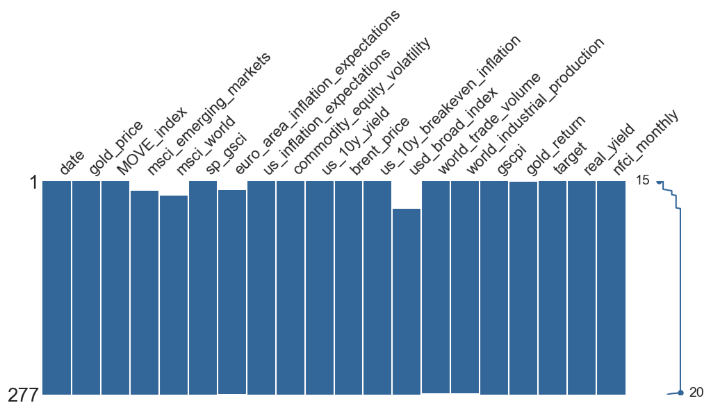

Several predictors contain missing values concentrated at the beginning of the sample. This pattern reflects data availability rather than stochastic missingness: some macro-financial series (such as the trade-weighted USD Broad Index or MSCI coverage) began being systematically recorded only after the early 2000s.

When missing values arise because a variable did not yet exist, the missingness is structural rather than stochastic. In such cases, imputing values would amount to fabricating observations that were never recorded, which can distort statistical relationships and artificially inflate the effective sample size. For this reason, imputation is not appropriate here.

The missingness pattern is easy to visualise:

missing_cols = [
    "usd_broad_index",
    "msci_world",
    "msci_emerging_markets",
    "euro_area_inflation_expectations"
]

plt.figure(figsize=(12, 3))
sns.heatmap(
    modelling_df[missing_cols].isna().T,
    cmap=["#2c7fb8", "#f03b20"],
    cbar=False
)
plt.title("All missingness confined to the start of the sample, i.e structural, not random")
plt.xlabel("Observation index")
plt.ylabel("Variables")
plt.show()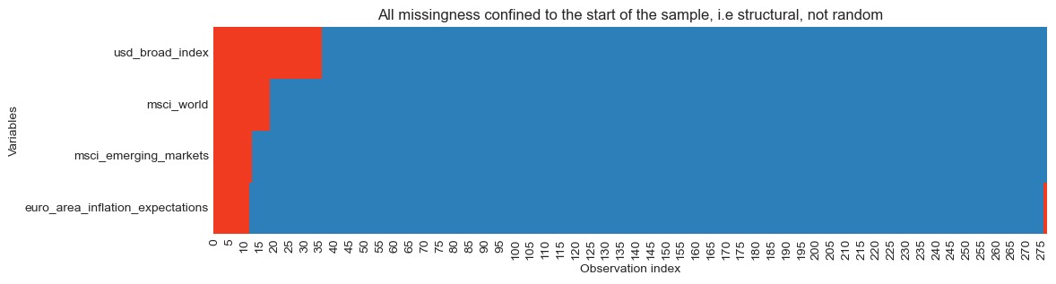

The heatmap confirms that missing observations occur only at the start of the dataset, confirming that this is a series start-date issue rather than random missing data. The missingness is best interpreted as MAR (Missing At Random) conditional on time (the probability of missingness depends on observation date, not on the gold return outcome).

Sample cost of including the USD index

Including predictors with missing values reduces the effective training sample, because rows containing missing predictors are removed during model fitting. To make this trade-off explicit, we compare the number of training observations available with and without the usd_broad_index variable (i.e the variable with the most missing values).

# 80/20 chronological split
split_idx = int(len(modelling_df) * 0.8)
train = modelling_df.iloc[:split_idx].copy()
test  = modelling_df.iloc[split_idx:].copy()

features_with_usd    = ['real_yield', 'usd_broad_index', 'nfci_monthly', 'MOVE_index', 'gscpi']
features_without_usd = ['real_yield', 'nfci_monthly', 'MOVE_index', 'gscpi']

n_with    = train[features_with_usd    + ['target']].dropna().shape[0]
n_without = train[features_without_usd + ['target']].dropna().shape[0]

print(f"Training obs WITH usd_broad_index:    {n_with} (dropped {len(train) - n_with})")
print(f"Training obs WITHOUT usd_broad_index: {n_without} (dropped {len(train) - n_without})")

Training obs WITH usd_broad_index:    185 (dropped 36)
Training obs WITHOUT usd_broad_index: 221 (dropped  0)

Including usd_broad_index removes the first 36 months of observations (2003–2005), reducing the effective training sample by about 16%.

Does the USD index add distinct information?

corr_usd = modelling_df.corr(numeric_only=True)['usd_broad_index'].sort_values()

fig, ax = plt.subplots(figsize=(9, 6))
colors = ['#c0392b' if c < 0 else '#27ae60' for c in corr_usd]
ax.barh(corr_usd.index, corr_usd.values, color=colors, edgecolor='white')
ax.axvline(0, color='black', linewidth=0.8)
ax.set_title('USD Broad Index has strong correlations with many features in the feature set',
             fontsize=11)
ax.set_xlabel('Pearson correlation with USD broad index')
plt.tight_layout()
plt.savefig('w08-correlations-usd.png', dpi=150)
plt.show()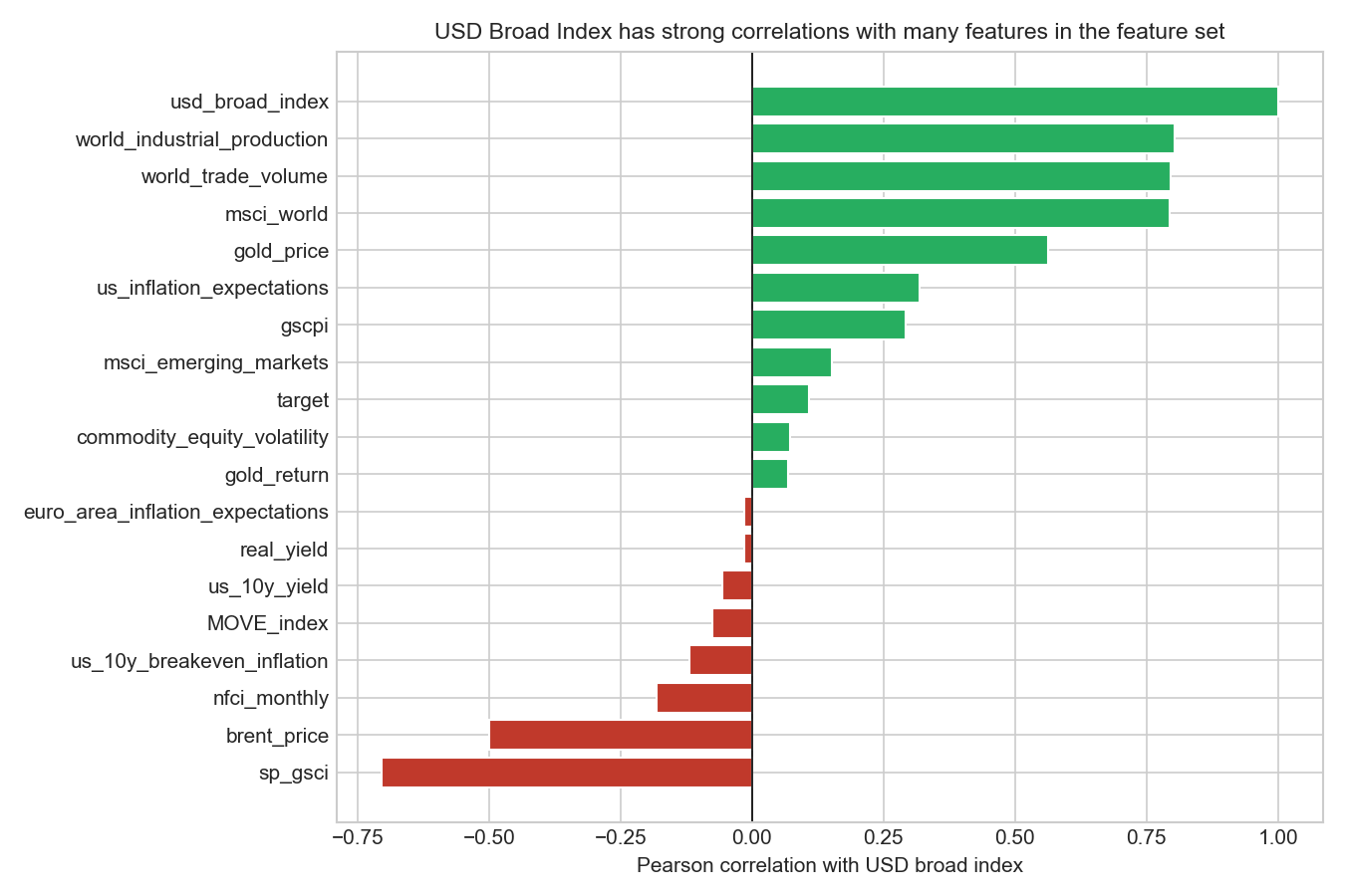

Before deciding whether to keep the variable, we examine whether the USD broad index contains information that is distinct from the rest of the feature set. Pairwise correlations show that the USD index is strongly related to several other predictors, especially msci_world, world_trade_volume, world_industrial_production, and sp_gsci, indicating substantial overlap with broader global macro-financial conditions. At the same time, its correlation with variables such as real_yield and nfci_monthly is relatively modest, so it is not simply a duplicate of any single predictor. Overall, the evidence suggests that the USD index may add some information, but much of its variation is already reflected elsewhere in the dataset. Given that retaining it would remove around 16% of available observations, we prioritise sample size and historical coverage over the potentially limited incremental signal from this variable.

Final feature decision

In this analysis we choose to exclude usd_broad_index from the baseline model.

Although the variable is theoretically relevant — gold is priced in USD and often moves inversely to the dollar —, the additional information it may provide is likely incremental rather than essential, while the sample loss it introduces is substantial.

Preserving the longer sample is particularly valuable in a time-series context, where the number of observations is limited and different macro-financial regimes may appear over time. The early-2000s period (2003–2006) corresponds to the pre-crisis expansion preceding the 2007–2008 financial turmoil, and retaining these observations allows the model to be estimated across a broader range of macroeconomic conditions.

This illustrates a common modelling trade-off in applied work: balancing theoretical completeness against sample size and data consistency. When predictors introduce structural missingness concentrated at the start of the sample, it is often preferable to prioritise the longest clean dataset unless the variable is essential for the research question.

1.4 Data exploration

Plot 1: Gold prices over time

fig, ax = plt.subplots(figsize=(12, 4))
ax.plot(modelling_df['date'], modelling_df['gold_price'], color='goldenrod', linewidth=1.8)
ax.set_title('Gold has gained nearly 12× in nominal value since 2003, with three distinct rally phases',
             fontsize=12)
ax.set_xlabel('Date')
ax.set_ylabel('Price (USD)')
ax.yaxis.set_major_formatter(mticker.FuncFormatter(lambda x, _: f'${x:,.0f}'))
plt.tight_layout()
plt.savefig('w08-gold-price.png', dpi=150)
plt.show()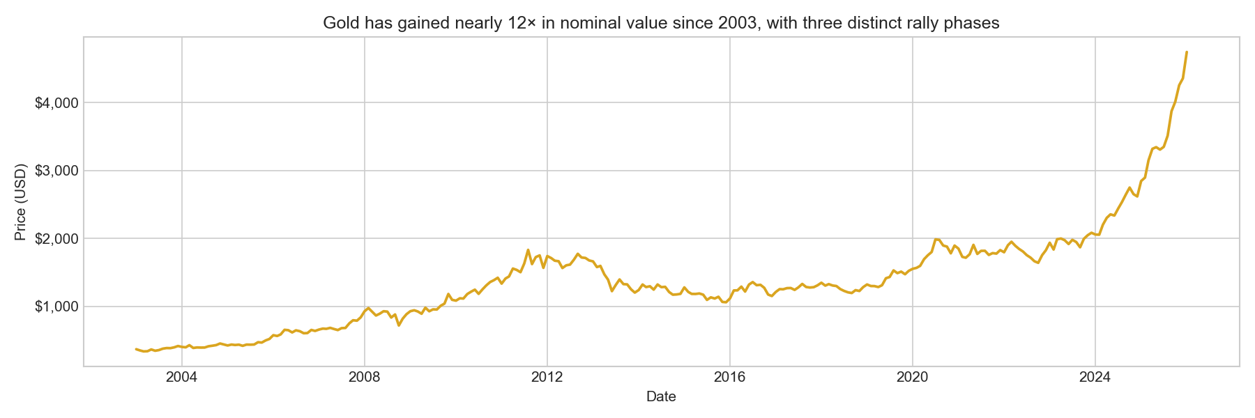

Gold has appreciated from roughly $370 in early 2003 to above $4,500 by early 2026, a nearly twelve-fold increase in nominal terms. Three major upswings are visible.

The 2008–2012 safe-haven rally was driven by the global financial crisis and its aftermath: quantitative easing, real yields turning deeply negative, and widespread loss of confidence in fiat currency. The 2018–2022 rally began with trade war anxiety and the Fed’s pivot toward easing, accelerated through the 2020 pandemic shock (when unprecedented monetary stimulus drove real yields to historic lows), and culminated in the 2022 inflation surge. The 2023–2026 surge is the most dramatic in the sample, driven by central bank gold-buying (especially from China and the Middle East), geopolitical risk following Russia’s invasion of Ukraine, and renewed concerns about reserve currency diversification.

This long-run trend reminds us that, while we are modelling returns (which are approximately stationary), the level series is clearly non-stationary. Working in return space is the right choice and avoids spurious regression.

Plot 2: Monthly gold returns

fig, ax = plt.subplots(figsize=(12, 4))
ax.bar(
    modelling_df['date'],
    modelling_df['gold_return'],
    color=['#c0392b' if r < 0 else '#27ae60' for r in modelling_df['gold_return']],
    width=20,
    alpha=0.8
)
ax.axhline(0, color='black', linewidth=0.8, linestyle='--')
ax.set_title('Monthly returns are approximately mean-zero with volatility clustering around crisis periods',
             fontsize=11)
ax.set_xlabel('Date')
ax.set_ylabel('Return (%)')
plt.tight_layout()
plt.savefig('w08-gold-returns.png', dpi=150)
plt.show()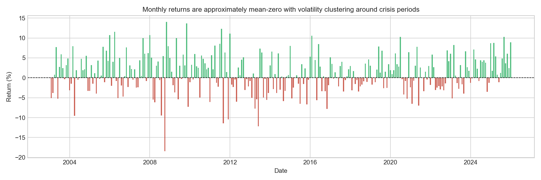

Monthly gold returns fluctuate around zero, with no clear long-run trend in the mean. This behaviour is typical of financial return series: while asset prices may trend over time, returns themselves are usually approximately mean-zero.

The series also exhibits clear volatility clustering, where large movements (both positive and negative) tend to occur close together, followed by periods of relatively small fluctuations. This pattern is a well-known stylised fact of financial markets and reflects the tendency of financial volatility to occur in bursts rather than being evenly distributed through time.

Several episodes of heightened activity are visible. In particular, the 2008–2009 global financial crisis and the 2011–2012 period surrounding the Eurozone sovereign-debt crisis and the peak of the gold market show sequences of unusually large monthly gains and losses. These clusters suggest that market turbulence tends to occur in bursts associated with major macro-financial events, rather than being evenly distributed through time. This has a direct implication for modelling: a linear regression trained on pooled data will estimate average relationships across different volatility regimes and will systematically underestimate the magnitude of returns during the most turbulent periods.

Plot 3: Rolling volatility

To examine how the variability of returns evolves over time, we compute a 12-month rolling standard deviation of monthly returns.

rolling_vol = modelling_df['gold_return'].rolling(12).std()

fig, ax = plt.subplots(figsize=(12, 4))
ax.plot(modelling_df['date'], rolling_vol, linewidth=2)

# Major crises
for start, end in [
    ('2008-09-01', '2009-07-01'),
    ('2011-08-01', '2012-10-01'),
    ('2020-03-01', '2021-06-01')
]:
    ax.axvspan(pd.Timestamp(start), pd.Timestamp(end), alpha=0.18, color='#F4C430')

# Secondary volatility episodes
secondary_periods = {
    ('2005-10-01', '2007-02-01'): 'Commodity boom',
    ('2012-12-01', '2013-07-01'): 'Gold crash',
    ('2015-10-01', '2016-05-01'): 'China slowdown',
    ('2018-03-01', '2019-10-01'): 'Trade tensions'
}
for (start, end), label in secondary_periods.items():
    ax.axvspan(pd.Timestamp(start), pd.Timestamp(end), alpha=0.04, color='steelblue')
    ax.text(pd.Timestamp(start), 0.6, label, fontsize=8, alpha=0.9)

ymax = rolling_vol.max()
ax.annotate("Global Financial Crisis",
    xy=(pd.Timestamp('2009-02-01'), ymax * 0.95),
    xytext=(pd.Timestamp('2006-06-01'), ymax * 1.05),
    arrowprops=dict(arrowstyle="->"), fontsize=9)
ax.annotate("Eurozone crisis / gold peak",
    xy=(pd.Timestamp('2012-01-01'), ymax * 0.82),
    xytext=(pd.Timestamp('2014-01-01'), ymax * 1.05),
    arrowprops=dict(arrowstyle="->"), fontsize=9)
ax.annotate("COVID market shock",
    xy=(pd.Timestamp('2021-02-01'), ymax * 0.55),
    xytext=(pd.Timestamp('2017-06-01'), ymax * 0.9),
    arrowprops=dict(arrowstyle="->"), fontsize=9)
ax.set_ylim(0, ymax * 1.15)
ax.set_title("Gold return volatility spikes during major financial shocks: three distinct crisis regimes visible",
             fontsize=11)
ax.set_xlabel("Date")
ax.set_ylabel("12-Month Rolling Std. Dev. of Returns")
ax.grid(axis='y', alpha=0.3)
plt.tight_layout()
plt.savefig('w08-rolling-vol.png', dpi=150)
plt.show()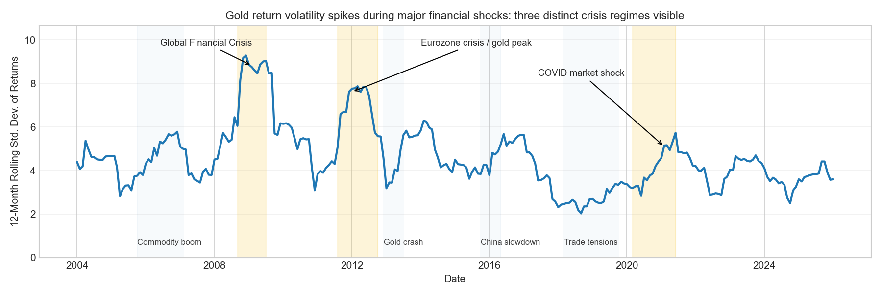

The rolling-volatility plot confirms that the return series is characterised by volatility regimes rather than a steady long-term trend.

Volatility rises sharply during the 2008–2009 global financial crisis, reaching its highest levels in the sample. A second pronounced spike occurs during the 2011–2012 Eurozone sovereign-debt crisis, which coincides with the peak of the gold market.

The plot also highlights several shorter episodes of elevated volatility linked to macro-financial developments, including the mid-2000s commodity boom, the 2013 gold market crash (triggered by the Fed’s “taper tantrum”), the 2015–2016 China growth slowdown, and the 2018–2019 US–China trade tensions. These periods illustrate that gold volatility often increases during times of global economic uncertainty.

After around 2014, volatility becomes more moderate, though temporary spikes still occur, most notably during the 2020 COVID-19 market shock.

This regime structure has a direct modelling implication: a linear regression trained on pooled data is estimating an average relationship across very different volatility environments, and the model’s errors will be disproportionately large during the volatile crisis periods i.e precisely the months that are most economically interesting. We will verify this explicitly when examining residuals in Section 1.5.3, where crisis-period residuals are expected to be visibly larger than those in calm periods.

Plot 4: Months with the largest absolute returns

top5 = modelling_df.nlargest(5, 'gold_return')[['date', 'gold_return']].copy()
bot5 = modelling_df.nsmallest(5, 'gold_return')[['date', 'gold_return']].copy()
extreme = pd.concat([top5, bot5]).sort_values('gold_return', ascending=False)
print(extreme.to_string(index=False))

      date  gold_return
2008-11-01    14.035088
2009-11-01    13.638985
2011-08-01    12.291564
2006-04-01    11.556162
2012-01-01    11.079908
2004-04-01    -9.526033
2011-12-01   -10.483917
2011-09-01   -11.432003
2013-06-01   -12.153625
2008-10-01   -18.460490

Date	Return (%)	Economic Context
Nov 2008	+14.0	Post-Lehman safe-haven surge: global credit markets frozen; investors fled to gold as systemic distrust of financial institutions peaked
Nov 2009	+13.6	QE-era rally: the Fed’s first round of quantitative easing drove real yields deeply negative and fuelled fears of dollar debasement
Aug 2011	+12.3	US debt ceiling standoff and S&P’s historic downgrade of US sovereign debt triggered a flight to gold as the ultimate safe-haven asset
Apr 2006	+11.6	Dollar weakness and rising commodity cycle; gold briefly broke through $600 for the first time since 1980
Jan 2012	+11.1	European sovereign debt crisis peak (Greece PSI negotiations), ECB LTRO announcement; real rates negative, investors sought inflation protection
Jun 2013	−12.2	“Taper tantrum”: Bernanke’s suggestion that the Fed might taper QE sent real yields surging, eliminating the key driver of gold’s post-2008 rally
Sep 2011	−11.4	Violent reversal after August’s peak; profit-taking and margin calls following gold’s near-$1,900 high; CME raised margin requirements
Dec 2011	−10.5	Dollar strengthening on Eurozone crisis contagion fears; year-end deleveraging and tax-loss harvesting
Oct 2008	−18.5	The single worst month in our sample: immediate post-Lehman liquidation panic. Gold was sold aggressively for cash as institutions faced margin calls — a temporary but violent reversal of its safe-haven role
Apr 2004	−9.5	Unexpectedly strong US non-farm payrolls raised rate hike expectations; dollar strengthened, gold sold off

These extreme observations reinforce the patterns visible in the volatility analysis. Most of the largest return movements occur during the 2008–2012 crisis period, when financial stress, central-bank interventions, and sharp shifts in real interest rates generated unusually turbulent market conditions.

Two mechanisms appear repeatedly. Safe-haven demand during systemic stress produces large positive gold returns. Rising real interest rates or liquidity shocks can trigger sharp sell-offs.

The most extreme observation — October 2008 (−18.5%) — highlights an important nuance: although gold is widely viewed as a safe-haven asset, it can still experience severe losses during acute liquidity crises when investors sell assets indiscriminately to raise cash.

These episodes emphasise the regime-dependent nature of gold returns, suggesting that different macroeconomic mechanisms may dominate in different periods, which is a fundamental challenge for any pooled linear model. Importantly, the predictors in our dataset (real yields, financial conditions, MOVE index) are precisely the variables that spiked or collapsed during these episodes. This motivates their inclusion in Section 1.5.2, and their appearance in the residuals during these months (large spikes in Section 1.5.3) is expected rather than a model failure.

Plot 5: Correlations with gold returns

Before constructing predictive models, we examine simple pairwise correlations between each predictor and next-month gold returns. This step is exploratory: correlations do not establish causality, but they provide a quick indication of which variables may contain useful signal.

all_predictors = ['real_yield', 'usd_broad_index', 'nfci_monthly', 'MOVE_index', 'gscpi',
                  'msci_world', 'msci_emerging_markets', 'brent_price',
                  'us_10y_breakeven_inflation', 'us_10y_yield',
                  'commodity_equity_volatility', 'us_inflation_expectations',
                  'euro_area_inflation_expectations', 'world_trade_volume',
                  'world_industrial_production', 'sp_gsci']

corr_all = modelling_df[['target'] + all_predictors].corr()['target'].drop('target').sort_values()

fig, ax = plt.subplots(figsize=(9, 6))
colors = ['#c0392b' if c < 0 else '#27ae60' for c in corr_all]
ax.barh(corr_all.index, corr_all.values, color=colors, edgecolor='white')
ax.axvline(0, color='black', linewidth=0.8)
ax.set_title('All macro predictors have weak bivariate correlations (|r| ≤ 0.22): no single variable dominates',
             fontsize=11)
ax.set_xlabel('Pearson Correlation')
plt.tight_layout()
plt.savefig('w08-correlations.png', dpi=150)
plt.show()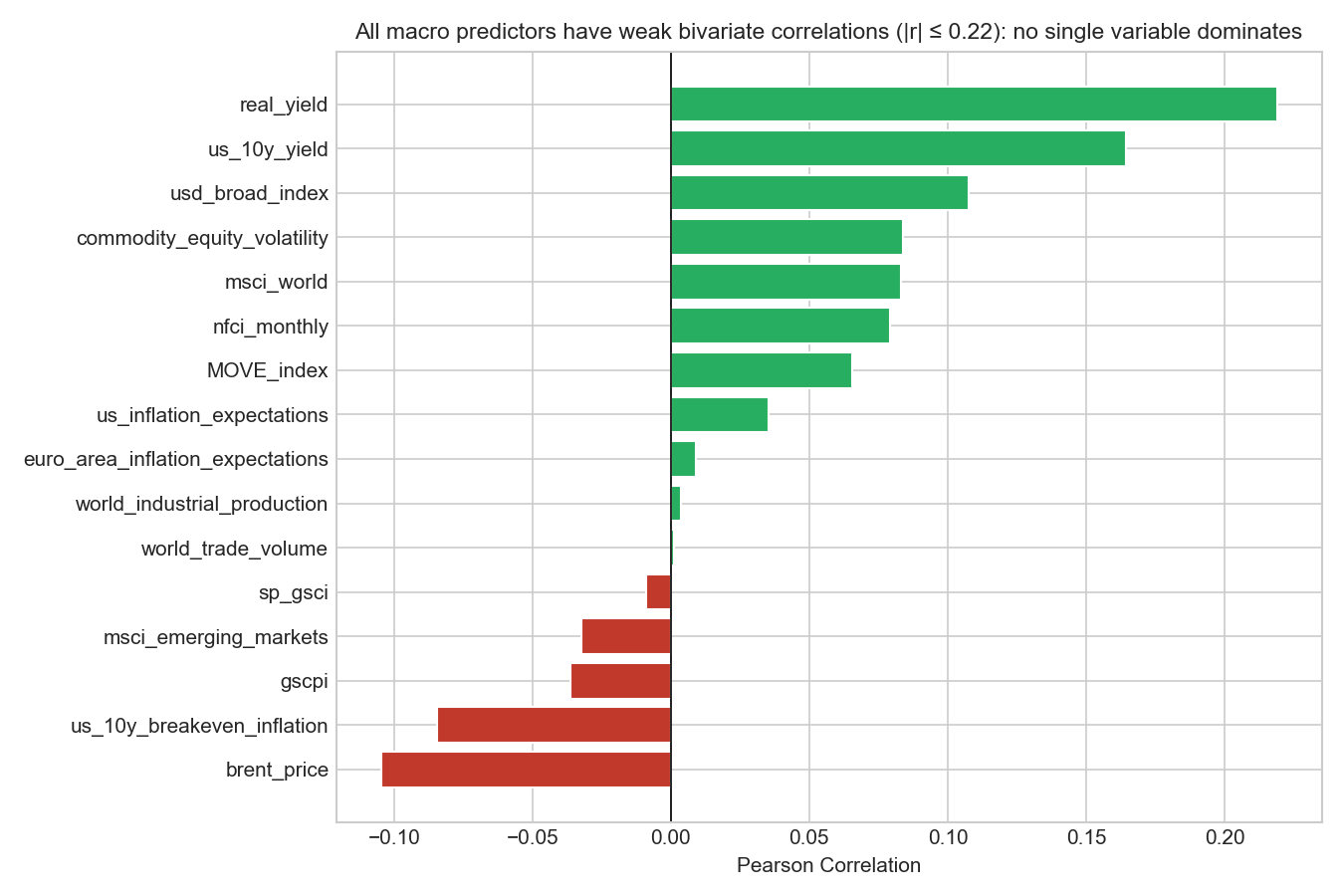

Overall strength of correlations

The first observation is that all correlations are relatively small, with absolute values below about 0.22. The strongest relationship is between real_yield and gold returns (r ≈ 0.22), followed by us_10y_yield (r ≈ 0.16) and usd_broad_index (r ≈ 0.11).

These modest values reinforce a key feature of financial markets: short-horizon asset returns are extremely noisy. Most month-to-month variation in gold returns cannot be explained by a single macroeconomic variable.

The real yield relationship

The strongest correlation is with real yields (r ≈ 0.22). Economic theory typically predicts a negative relationship between real interest rates and gold prices, because gold does not pay interest. When real yields rise, investors can earn higher inflation-adjusted returns on bonds, making gold relatively less attractive. However, the positive correlation observed here likely reflects specific macroeconomic episodes in the sample. During 2019–2020, gold prices rose strongly even as real yields increased due to large fiscal stimulus and financial uncertainty. During some tightening cycles, rising interest rates coincided with broader commodity price rallies or currency movements that supported gold. These examples illustrate an important statistical point: bivariate correlations can mask more complex relationships that depend on the broader macroeconomic environment. The sign of the coefficient in a multivariate model may differ from the bivariate correlation.

Financial stress indicators

Variables measuring financial stress show small but positive correlations with gold returns: nfci_monthly (r ≈ 0.08) and MOVE_index (r ≈ 0.06). Although these relationships are weak, they are consistent with gold’s reputation as a partial safe-haven asset. When financial conditions tighten or market volatility rises, investors sometimes shift toward assets perceived as stores of value, including gold. However, the correlations are small because this relationship does not hold in all situations. In severe liquidity crises such as October 2008, gold can actually fall as investors sell assets to raise cash.

Commodity and inflation variables

Some variables show small negative correlations with gold returns, such as brent_price (r ≈ −0.10) and us_10y_breakeven_inflation (r ≈ −0.08). These values are small enough that they should not be interpreted as strong economic relationships. Instead, they likely reflect sample-specific dynamics, such as periods when oil prices rose due to supply shocks while gold prices moved differently. The key takeaway is that inflation-related variables do not appear to provide strong short-horizon predictive power for gold returns in this dataset, despite the common narrative that gold acts as an inflation hedge.

Checking for multicollinearity among predictors

Before estimating models, we examine whether some predictors are strongly correlated with each other, which can lead to multicollinearity, inflated coefficient variance and unstable estimates.

predictors_for_corr = ['real_yield', 'nfci_monthly', 'MOVE_index', 'gscpi',
                       'usd_broad_index', 'us_10y_yield', 'msci_world',
                       'brent_price', 'us_10y_breakeven_inflation',
                       'commodity_equity_volatility', 'us_inflation_expectations',
                       'world_trade_volume', 'world_industrial_production', 'sp_gsci']

corr_matrix = modelling_df[predictors_for_corr].corr()
mask = np.triu(np.ones_like(corr_matrix, dtype=bool))

fig, ax = plt.subplots(figsize=(10, 8))
sns.heatmap(
    corr_matrix, mask=mask, cmap="coolwarm",
    vmin=-1, vmax=1, center=0,
    annot=True, fmt=".2f", linewidths=0.5,
    cbar_kws={"shrink": .8}, ax=ax
)
ax.set_title("Several clusters of correlated predictors, including near-perfect collinearity in activity indices")
plt.tight_layout()
plt.savefig('w08-predictor-corr-matrix.png', dpi=150)
plt.show()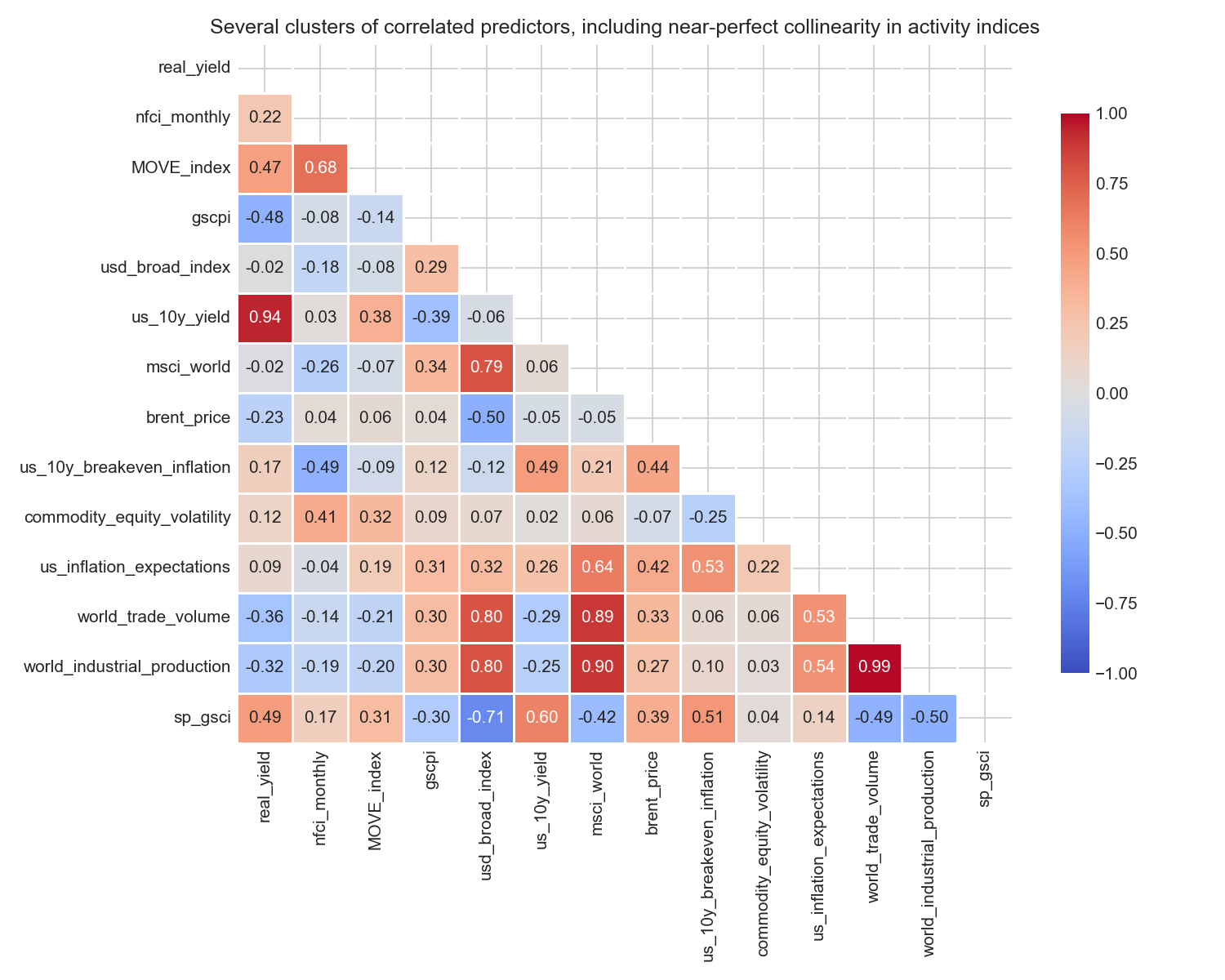

The heatmap reveals several important clusters.

Interest-rate variables: real_yield and us_10y_yield are very strongly correlated (r ≈ 0.94). This is expected: real yield is derived directly from nominal yield by subtracting breakeven inflation. Including both would be severely redundant. We retain real_yield as the economically more meaningful measure.

Financial stress: MOVE_index and nfci_monthly are substantially correlated (r ≈ 0.75). Both measure aspects of financial market stress; NFCI is the more comprehensive composite. The moderate (not extreme) correlation means we can include both without severe multicollinearity, as confirmed by the VIF analysis below.

Global economic activity: world_trade_volume and world_industrial_production are almost perfectly correlated (r ≈ 0.99); they are measuring the same global business cycle. Including both would be completely redundant. MSCI World is also highly correlated with both (r ≈ 0.90), confirming they all capture the same underlying growth signal.

Commodity cycles: brent_price and sp_gsci show a moderate positive correlation (~0.39), both reflecting commodity price movements. Neither shows strong correlation with the target.

These clusters directly motivate our parsimonious feature set: we select at most one variable from each strongly correlated group, prioritising theoretical relevance and coverage of distinct economic channels.

Summary of the correlation analysis

The correlation analysis highlights three important points:

Predictive relationships are weak. No single macroeconomic indicator strongly predicts next-month gold returns.
Some economic signals exist. Real yields, financial conditions, and currency movements show modest relationships with gold returns.
Relationships are context-dependent. The sign and strength of correlations may change across different macroeconomic regimes.

For these reasons, correlations should be viewed as exploratory diagnostics rather than definitive evidence of predictive relationships. Variables with weak pairwise correlations may still contribute useful information when combined in a multivariate model, particularly when they capture different dimensions of the macroeconomic environment. The correlation analysis also serves as the first filter in our feature selection workflow in Section 1.5.2: predictors with very weak bivariate correlations (|r| < 0.05) and no compelling theoretical rationale will be dropped there as part of the iterative VIF-based pruning process.

Plot 6: Multi-variable visualisation

plot_df = modelling_df[['date', 'target', 'real_yield', 'usd_broad_index', 'nfci_monthly']].dropna()

fig, axes = plt.subplots(1, 2, figsize=(14, 5))

sc = axes[0].scatter(plot_df['real_yield'], plot_df['target'],
                     c=plot_df['usd_broad_index'], cmap='RdYlGn_r',
                     alpha=0.7, edgecolors='grey', linewidths=0.3, s=40)
plt.colorbar(sc, ax=axes[0], label='USD Broad Index')
axes[0].axhline(0, color='black', linewidth=0.7, linestyle='--')
axes[0].axvline(0, color='black', linewidth=0.7, linestyle='--')
axes[0].set_xlabel('Real Yield (10Y Nominal − Breakeven, %)')
axes[0].set_ylabel('Next-Month Gold Return (%)')
axes[0].set_title('Negative real yields associate with positive gold returns;\nbut the relationship is noisy and regime-dependent',
                  fontsize=9)

sc2 = axes[1].scatter(plot_df['nfci_monthly'], plot_df['target'],
                      c=plot_df['real_yield'], cmap='coolwarm',
                      alpha=0.7, edgecolors='grey', linewidths=0.3, s=40)
plt.colorbar(sc2, ax=axes[1], label='Real Yield (%)')
axes[1].axhline(0, color='black', linewidth=0.7, linestyle='--')
axes[1].set_xlabel('NFCI (monthly mean)')
axes[1].set_ylabel('Next-Month Gold Return (%)')
axes[1].set_title('Largest gold rallies occur when financial conditions are tight\nand real rates are low (blue dots)',
                  fontsize=9)

plt.tight_layout()
plt.savefig('w08-gold-multivariable-plot.png', dpi=150)
plt.show()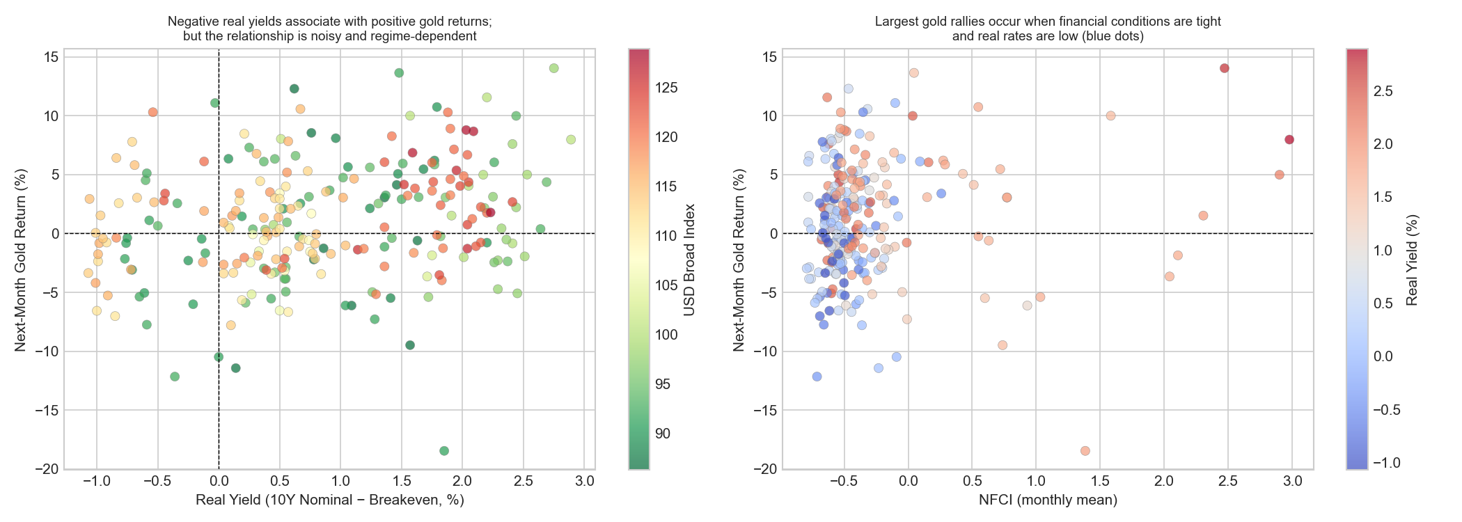

These plots extend the earlier correlation analysis by examining how gold returns behave when multiple macro variables interact simultaneously.

Real yields, the US dollar, and gold returns

The left panel plots real yields against next-month gold returns, with the colour of each point representing the strength of the US dollar.

The scatter shows substantial dispersion, confirming that the relationship between real yields and gold returns is weak. Even when real yields are very low or negative, gold returns can vary widely. This reinforces the conclusion from the correlation analysis that no single macro variable provides strong predictive power for monthly gold returns.

The colour scale reveals that movements in gold returns often coincide with changes in the US dollar. Many observations with positive gold returns are associated with lighter green colours, indicating periods when the dollar was relatively weak. This suggests that some of the apparent relationship between real yields and gold returns may actually reflect interactions between interest rates and currency movements, a reminder that, when multiple forces operate simultaneously, simple pairwise correlations can give a misleading picture.

There is also a visible concentration of observations in the upper-left quadrant (negative real yields and positive gold returns). This pattern is consistent with the theoretical view that gold performs well when real interest rates are low or negative, because the opportunity cost of holding a non-interest-bearing asset decreases.

Financial conditions and safe-haven behaviour

The right panel shows the relationship between financial conditions (nfci_monthly) and gold returns, while the colour scale now represents real yields.

Most observations cluster around moderate financial conditions and near-zero returns. However, some of the largest positive gold returns appear when financial conditions tighten sharply. The colour scale provides additional insight: many of the strongest positive gold returns occur when financial conditions are tight and real yields are relatively low (blue-coloured points). This combination is typical of periods of financial stress, when investors seek assets perceived as safe stores of value.

Linking the multivariate view to the earlier diagnostics

Taken together, these plots help reconcile several findings from the previous analysis. Gold returns are influenced by multiple macroeconomic forces simultaneously: interest rates, currency movements, financial stress, and commodity market dynamics. When these factors interact, simple pairwise statistics may not capture the full structure of the relationships. This observation reinforces an important point for the modelling stage: predictive relationships are likely to be multivariate and regime-dependent, rather than driven by a single macroeconomic variable. It also foreshadows why the LightGBM model in Section 1.5.4, despite its flexibility to capture interactions, does not substantially outperform the linear baseline. The joint non-linear structure visible in these plots is real, but not consistent enough across time windows to be reliably exploited with 221 training observations.

Implications for modelling

These observations highlight an important challenge for predictive modelling.

Monthly gold returns are noisy and centred around zero, meaning that most of the variation in the series is difficult to explain using simple linear relationships. The volatility analysis reveals that market behaviour changes across distinct macro-financial regimes, with periods of heightened turbulence associated with major economic shocks and policy uncertainty.

The correlation diagnostics further suggest that, while several macro-financial variables contain modest predictive signal, many predictors are also correlated with each other, reflecting overlapping economic information.

Taken together, these findings imply that predictive performance may be limited and that modelling results should be interpreted cautiously. Nevertheless, macro-financial indicators may still provide partial information about the economic environment in which gold returns are generated. The modelling exercise that follows should therefore be viewed as an exploratory attempt to extract any systematic signal from these macro indicators, rather than an expectation that gold returns can be forecast with high precision.

1.5 Modelling

1.5.1 Train/test split

# Ensure chronological ordering
modelling_df = modelling_df.sort_values('date').reset_index(drop=True)

# Temporal 80/20 split
split_idx = int(len(modelling_df) * 0.8)
train = modelling_df.iloc[:split_idx].copy()
test  = modelling_df.iloc[split_idx:].copy()

print(f"Training: {train['date'].min().date()} to {train['date'].max().date()} ({len(train)} obs)")
print(f"Test:     {test['date'].min().date()} to {test['date'].max().date()} ({len(test)} obs)")

Training: 2003-01-01 to 2021-05-01 (221 obs)
Test:     2021-06-01 to 2026-01-01 (56 obs)

Justification

Because the dataset is a time series, the training and test sets must respect the chronological order of observations. Random cross-validation would mix past and future observations, allowing the model to learn from information that would not have been available at the time predictions were made, a classic form of data leakage.

We therefore use a strict temporal split, training the model on earlier observations and evaluating its performance on later data.

Using an 80/20 chronological split ensures that:

the model is trained on the majority of the available historical data,
the test set remains a genuinely unseen out-of-sample period, and
the evaluation reflects the model’s ability to generalise to new macro-financial conditions.

The test set (June 2021–January 2026) is particularly demanding: it covers the post-pandemic commodity rally, the 2022 inflation surge and the most aggressive Fed tightening cycle in 40 years, and elevated geopolitical risk following Russia’s invasion of Ukraine. This is a genuine test of whether the relationships estimated on the pre-2021 sample generalise to a structurally different macro regime.

The test set is not used for any modelling decisions. It is reserved solely for final performance evaluation.

1.5.2 Feature selection

The dataset contains a fairly large number of macro-financial indicators, and many of them capture related underlying economic forces, e.g interest-rate conditions, global activity, inflation pressures, commodity cycles, and financial market stress. Including all available predictors simultaneously therefore risks multicollinearity, where predictors contain overlapping information. Multicollinearity can inflate standard errors, make coefficient estimates unstable and difficult to interpret, and weaken out-of-sample performance.

Feature selection therefore proceeds in three steps:

Structural filtering: predictors that are mechanically derived from variables already included are dropped first. For example, us_10y_yield and us_10y_breakeven_inflation are excluded because real_yield already combines them.
Sample-cost filtering: usd_broad_index is excluded as discussed in Section 1.3.4. Although economically relevant, it would substantially reduce the usable sample because of missing early observations.
Multicollinearity diagnostics (VIF): we compute VIFs on the remaining candidate set and iteratively remove redundant predictors, re-checking after each round until the remaining set is acceptably stable.

Step 1 & 2: Structural filtering and candidate set

After the above exclusions, the initial candidate predictor set is:

candidate_features = [
    'MOVE_index', 'msci_emerging_markets', 'msci_world', 'sp_gsci',
    'euro_area_inflation_expectations', 'us_inflation_expectations',
    'commodity_equity_volatility', 'brent_price', 'world_trade_volume',
    'world_industrial_production', 'gscpi', 'real_yield', 'nfci_monthly'
]

Step 3: Iterative VIF pruning

def compute_vif(df, features):
    vif_data = df[features].dropna()
    return pd.DataFrame({
        "feature": features,
        "VIF": [variance_inflation_factor(vif_data.values, i)
                for i in range(len(features))]
    }).sort_values("VIF", ascending=False)

# Round 1: VIF on full candidate set
print("=== Round 1: Full candidate set ===")
print(compute_vif(train, candidate_features).round(2).to_string(index=False))

=== Round 1: Full candidate set ===
                         feature     VIF
              world_trade_volume 4124.51
     world_industrial_production 3483.54
                      msci_world  130.95
           msci_emerging_markets  114.44
       us_inflation_expectations  101.86
                     brent_price   69.10
                         sp_gsci   65.46
                      MOVE_index   40.18
euro_area_inflation_expectations   12.91
     commodity_equity_volatility   11.62
                      real_yield    5.91
                    nfci_monthly    5.08
                           gscpi    2.58

The full candidate set shows extreme multicollinearity. The clearest redundancy appears in three blocks. First, the global-cycle block — world_trade_volume, world_industrial_production, msci_world, and msci_emerging_markets — contains several variables that all move with the same broad world business cycle. Second, the commodity block — brent_price and sp_gsci — contains two closely related measures of commodity-market conditions. Third, the inflation-expectations block — us_inflation_expectations and euro_area_inflation_expectations — risks overlapping both with each other and with real_yield.

We begin by pruning the commodity block.

# Round 2: Remove brent_price
cands_r2 = [f for f in candidate_features if f != 'brent_price']
print("\n=== Round 2: After removing brent_price ===")
print(compute_vif(train, cands_r2).round(2).to_string(index=False))

=== Round 2: After removing brent_price ===
                         feature     VIF
              world_trade_volume 3455.07
     world_industrial_production 3030.78
       us_inflation_expectations   94.12
           msci_emerging_markets   85.11
                      msci_world   77.00
                         sp_gsci   58.96
                      MOVE_index   39.91
euro_area_inflation_expectations   11.90
     commodity_equity_volatility   10.96
                    nfci_monthly    5.06
                      real_yield    4.90
                           gscpi    2.53

brent_price is removed first because it is the narrower of the two commodity proxies. sp_gsci is retained at this stage because it is broader and better aligned with a general commodity-cycle interpretation, whereas brent_price is more oil-specific.

The next step is to collapse the global-cycle block by removing variables that duplicate the same underlying world business-cycle signal.

# Round 3: Collapse the global-cycle block
cands_r3 = [
    'MOVE_index', 'msci_world', 'sp_gsci',
    'euro_area_inflation_expectations', 'us_inflation_expectations',
    'commodity_equity_volatility', 'gscpi', 'real_yield', 'nfci_monthly'
]
print("\n=== Round 3: After collapsing the global cycle block ===")
print(compute_vif(train, cands_r3).round(2).to_string(index=False))

=== Round 3: After collapsing the global cycle block ===
                         feature   VIF
       us_inflation_expectations 77.35
                         sp_gsci 45.37
                      MOVE_index 27.62
                      msci_world 23.03
euro_area_inflation_expectations 10.67
     commodity_equity_volatility  9.95
                    nfci_monthly  4.15
                      real_yield  3.92
                           gscpi  1.56

In this round, world_trade_volume, world_industrial_production, and msci_emerging_markets are removed. The first two both proxy global real activity, while msci_emerging_markets overlaps strongly with msci_world. We retain msci_world as the broadest and cleanest representative of global market conditions. This substantially reduces the most extreme collinearity, but the model is still unstable: us_inflation_expectations, sp_gsci, MOVE_index, and msci_world all remain highly collinear.

We next address the inflation-expectations block.

# Round 4a: Remove euro-area inflation expectations
cands_r4a = [f for f in cands_r3 if f != 'euro_area_inflation_expectations']
print("\n=== Round 4: After removing inflation expectations (EU) ===")
print(compute_vif(train, cands_r4a).round(2).to_string(index=False))

=== Round 4: After removing inflation expectations (EU) ===
                    feature   VIF
  us_inflation_expectations 77.26
                    sp_gsci 36.60
                 MOVE_index 24.13
                 msci_world 21.46
commodity_equity_volatility  9.09
               nfci_monthly  4.08
                 real_yield  3.75
                      gscpi  1.50

euro_area_inflation_expectations is removed first because, in a USD gold-pricing setting, it is less central than the US measure. However, this change barely affects the collinearity problem: us_inflation_expectations remains extremely high.

We therefore remove the US inflation-expectations series as well.

# Round 4b: Remove US inflation expectations
cands_r4b = [f for f in cands_r4a if f != 'us_inflation_expectations']
print("\n=== Round 4: After removing inflation expectations (US) ===")
print(compute_vif(train, cands_r4b).round(2).to_string(index=False))

=== Round 4: After removing inflation expectations (US) ===
                    feature   VIF
                 MOVE_index 22.22
                 msci_world 13.32
                    sp_gsci 11.73
commodity_equity_volatility  9.02
               nfci_monthly  3.85
                 real_yield  3.19
                      gscpi  1.47

This confirms that the inflation-expectations variables were contributing substantial redundancy. Once they are removed, the model is much improved, but not yet fully stable: MOVE_index, msci_world, and sp_gsci still remain above the threshold of 10.

The final pruning step is therefore a stabilisation round.

# Round 5: Remove sp_gsci and MOVE_index
cands_r5 = [
    'msci_world', 'commodity_equity_volatility',
    'real_yield', 'nfci_monthly', 'gscpi'
]
print("\n=== Round 5: After removing sp_gsci and MOVE_index ===")
print(compute_vif(train, cands_r5).round(2).to_string(index=False))

=== Round 5: After removing sp_gsci and MOVE_index ===
                    feature  VIF
                 msci_world 8.32
commodity_equity_volatility 7.17
                 real_yield 2.12
               nfci_monthly 2.03
                      gscpi 1.27

At this stage, all remaining VIFs are below 10, so the iterative pruning process stops here.

This leaves the following final feature set:

candidate_features_final = [
    'msci_world',
    'commodity_equity_volatility',
    'real_yield',
    'nfci_monthly',
    'gscpi'
]

print("\n=== Final candidate set ===")
print(compute_vif(train, candidate_features_final).round(2).to_string(index=False))

=== Final candidate set ===
                    feature  VIF
                 msci_world 8.32
commodity_equity_volatility 7.17
                 real_yield 2.12
               nfci_monthly 2.03
                      gscpi 1.27

The final retained predictors capture five economically distinct channels relevant to gold returns:

real_yield: the opportunity cost of holding gold relative to inflation-protected bonds
nfci_monthly: broad financial conditions, including credit and liquidity stress
gscpi: global supply-chain pressure and the broader supply-side inflation environment
msci_world: global equity-market conditions and investor risk sentiment
commodity_equity_volatility: uncertainty in commodity-linked equity markets, capturing an additional dimension of resource-sector risk

Two variables that were initially attractive on theoretical grounds (MOVE_index and sp_gsci) do not survive the final specification because, after the earlier pruning rounds, they still remain too strongly entangled with the broader market-stress and commodity/global-cycle structure. Retaining them would therefore add instability without enough distinct information to justify their inclusion.

Importantly, the decision to stop at 5 predictors is not driven by sample size alone. The training set contains 221 observations, so even a model with 10 predictors would still have about 22 observations per predictor, and a model with 12 predictors would still have about 18 observations per predictor. Those ratios are not automatically problematic. However, feature selection is not only about satisfying a minimum observations-to-predictor rule. In a relatively small macro-financial time-series setting, adding more variables that are strongly related to one another can reduce stability and make the model harder to interpret without adding much incremental signal.

For that reason, 5 predictors is a reasonable middle ground: small enough to avoid the severe redundancy seen in the full candidate set, but still rich enough to retain several distinct economic channels.

With 5 predictors on 221 training observations, the observation-to-predictor ratio is 44.2:1, which remains comfortably conservative.

1.5.3 Baseline linear regression

We begin with an ordinary least squares (OLS) regression as a baseline forecasting model.

Linear models provide a useful starting point because they are transparent, easy to interpret, and widely used as benchmarks in macro-financial forecasting. Even if the true relationship between macro variables and gold returns is nonlinear, a linear specification allows us to test whether the selected macro-financial indicators contain any systematic predictive signal.

features = candidate_features_final

train_clean = train[features + ['target']].dropna()
test_clean  = test[features  + ['target']].dropna()

X_train = train_clean[features]
y_train = train_clean['target']
X_test  = test_clean[features]
y_test  = test_clean['target']

lr = LinearRegression()
lr.fit(X_train, y_train)

y_pred_train = lr.predict(X_train)
y_pred_test  = lr.predict(X_test)

Evaluation metrics

Forecast accuracy is evaluated using three complementary metrics.

R² (Coefficient of Determination): R² measures the proportion of variance in the target variable explained by the model. In financial return forecasting, R² values are typically very small, because short-horizon asset returns are dominated by unpredictable news and market shocks. A negative out-of-sample R² indicates that the model performs worse than a historical mean forecast, which serves as a natural baseline benchmark.

Mean Absolute Error (MAE): MAE measures the average absolute forecast error in percentage points of return. Because financial returns occasionally exhibit large shocks, MAE provides a robust measure of the typical prediction error.

Root Mean Squared Error (RMSE): RMSE penalises large errors more heavily than MAE because errors are squared before averaging. This metric is therefore sensitive to large forecasting mistakes during crisis periods, which are economically important in financial markets.

def evaluate(y_true, y_pred, label):
    r2   = r2_score(y_true, y_pred)
    mae  = mean_absolute_error(y_true, y_pred)
    rmse = np.sqrt(mean_squared_error(y_true, y_pred))
    print(f"{label}: R²={r2:.4f}, MAE={mae:.4f}%, RMSE={rmse:.4f}%")

evaluate(y_train, y_pred_train, "Train")
evaluate(y_test,  y_pred_test,  "Test ")

Train: R²=0.0490, MAE=3.8366%, RMSE=4.9046%
Test : R²=0.1383, MAE=3.0510%, RMSE=3.5693%

Comparison with a naïve forecast

To evaluate whether the regression model adds value, we compare it to a simple naïve benchmark that predicts the historical mean return every month.

mean_train = y_train.mean()
y_pred_naive = np.full(len(y_test), mean_train)
print(f"Training mean return: {mean_train:.4f}%")
evaluate(y_test, y_pred_naive, "Naive")

Training mean return: 0.8506%
Naive: R²=-0.0752, MAE=3.3639%, RMSE=3.9871%

Model	Test R²	Test MAE	Test RMSE
Naïve (historical mean)	−0.075	3.36%	3.99%
OLS baseline	+0.138	3.05%	3.57%

The regression model outperforms the naïve forecast across all three evaluation metrics. Relative to the historical-mean benchmark, it reduces the mean absolute error from 3.36% to 3.05% and the root mean squared error from 3.99% to 3.57%, while also achieving a positive out-of-sample $R^2$ of 0.138. Because the target variable is the monthly gold return measured in percentage points, these errors can be read directly on the scale of the outcome: on average, the model’s predictions miss the realised next-month return by about 3.05 percentage points, and larger misses are substantial enough to produce an RMSE of 3.57 percentage points. An MAE of 3.05 percentage points is non-trivial given that monthly gold returns themselves are often only a few percentage points in magnitude.

This suggests that the selected macro-financial variables contain some genuine predictive information about next-month gold returns, since the model improves consistently on the historical-mean benchmark. However, the gains remain modest. In practical terms, the model is somewhat better at forecasting monthly returns than simply predicting the average, but forecast errors are still large relative to the scale of month-to-month gold-price movements. The results should therefore be interpreted as evidence of limited but real predictive value, rather than strong forecasting power.

Adjusted R²

Because the regression model includes several predictors, it is useful to compute the adjusted R², which penalises the inclusion of unnecessary variables.

n, p = len(X_train), len(features)
adj_r2_train = 1 - (1 - r2_score(y_train, y_pred_train)) * (n - 1) / (n - p - 1)
print(f"Adjusted R² (train): {adj_r2_train:.4f}")

Adjusted R² (train): 0.0247

The adjusted R² of 0.0247 is smaller than the raw in-sample R² of 0.049, reflecting the penalty for using 5 predictors on 221 observations. The model explains less than 5% of gold return variation in the training period. This is a key finding: macro indicators explain very little of month-to-month gold return variance, consistent with the near-efficiency of commodity futures markets.

Coefficient interpretation

coef_df = pd.DataFrame({'Feature': features, 'Coefficient': lr.coef_})
coef_df = coef_df.reindex(coef_df['Coefficient'].abs().sort_values(ascending=False).index)
print(coef_df.to_string(index=False))
print(f"\nIntercept: {lr.intercept_:.4f}")

                    Feature  Coefficient
                 real_yield     1.207170
                      gscpi     0.342028
               nfci_monthly     0.285436
commodity_equity_volatility     0.024486
                 msci_world     0.000333

Intercept: -0.7898

We interpret each coefficient as the predicted change in next-month gold return (in percentage points) associated with a one-unit increase in the predictor, holding the other included predictors constant. Because these predictors are measured in different units, the coefficients are most informative for their sign and conditional role in the model, rather than as directly comparable effect sizes. More broadly, these are conditional predictive associations, not isolated causal effects.

Feature	Coefficient	Economic Interpretation
`real_yield`	+1.21	A 1 percentage point increase in real yield is associated with a 1.21 percentage point increase in next-month gold return, holding the other predictors fixed. This sign is counterintuitive relative to standard theory, which would usually predict a negative relationship because higher real yields raise the opportunity cost of holding gold. In this sample, however, `real_yield` appears to be capturing more than the textbook opportunity-cost channel. In particular, some high-real-yield observations occur in stressed macro-financial environments or in the aftermath of major shocks, when gold subsequently performed strongly. In the multivariable regression, `real_yield` may therefore be acting partly as a broader regime indicator rather than a pure measure of carrying cost. This coefficient should be interpreted cautiously.
`gscpi`	+0.34	Higher global supply-chain pressure is associated with slightly higher next-month gold returns. This is directionally consistent with the idea that supply disruptions raise inflationary pressure and macro uncertainty, both of which can support demand for gold. The coefficient is positive and economically plausible, though modest in size.
`nfci_monthly`	+0.29	Tighter financial conditions are associated with slightly higher next-month gold returns. This is consistent with gold’s safe-haven role: when credit conditions deteriorate and broader financial stress rises, demand for defensive assets may increase. The effect is not large, but the sign is theoretically sensible.
`commodity_equity_volatility`	+0.02	The coefficient is very small, suggesting that commodity-linked equity volatility adds little incremental predictive power once broader financial conditions, supply-chain pressure, and real yields are already controlled for. Its positive sign is not implausible.Greater uncertainty in commodity-related sectors could coincide with stronger demand for real assets, but its contribution appears limited.
`msci_world`	+0.0003	The coefficient is positive but economically tiny on its raw scale, indicating that global equity-market conditions add very little marginal predictive signal once the other macro-financial variables are already in the model. In practice, this variable may still help absorb some broad market-cycle variation, but the coefficient suggests only a minimal direct association with next-month gold returns in this specification.

The intercept is −0.7898, meaning that when all predictors are set to zero, the model predicts a next-month gold return of about −0.79 percentage points. Because zero is not necessarily a substantively meaningful value for every predictor, the intercept is mainly a calibration term rather than an economically important parameter.

Flag on counterintuitive signs: The positive coefficient on real_yield goes against the usual theoretical expectation and should not be over-interpreted. Rather than invalidating the model, it suggests that simple macro levels may proxy broader crisis or regime conditions, especially in a relatively small historical sample. This is an important reminder that predictive regression coefficients in macro-financial settings do not always map cleanly onto textbook comparative statics.

Predicted vs actual returns

fig, axes = plt.subplots(1, 2, figsize=(12, 5))

for ax, y_true, y_pred, title in [
    (axes[0], y_train, y_pred_train, "Training"),
    (axes[1], y_test,  y_pred_test,  "Test")
]:
    ax.scatter(y_pred, y_true, alpha=0.7)
    min_val = min(y_true.min(), y_pred.min())
    max_val = max(y_true.max(), y_pred.max())
    ax.plot([min_val, max_val], [min_val, max_val], linestyle="--", color='red')
    ax.set_xlabel("Predicted Return (%)")
    ax.set_ylabel("Actual Return (%)")
    ax.set_title(f"Model predictions span a narrow band; actual returns span much wider: {title}",
                 fontsize=9)

plt.tight_layout()
plt.savefig('w08-gold-baseline-predicted-vs-actual.png', dpi=150)
plt.show()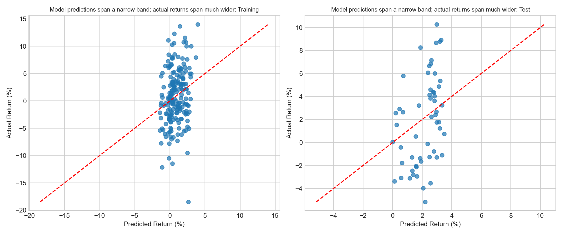

Several patterns are visible.

First, predicted returns lie in a much narrower range than actual returns. While realised monthly gold returns range roughly from −18% to +14%, the model’s predictions cluster between approximately −2% and +5%. This behaviour is typical in financial forecasting: because extreme market movements are usually driven by unexpected events, macro-financial predictors explain only a small portion of return variation.

Second, the points are broadly aligned with the 45-degree line, indicating that higher predicted returns tend to correspond to higher realised returns, although the relationship remains weak. The positive out-of-sample R² of 0.138 confirms that the model extracts a genuine signal, even if it cannot predict the magnitude of extreme events.

Residual analysis

# Build aligned residual tables from the cleaned samples actually used by the model
train_results = train_clean.copy()
train_results["date"] = train.loc[train_clean.index, "date"].values
train_results["y_true"] = y_train.values
train_results["y_pred"] = y_pred_train
train_results["residual"] = train_results["y_true"] - train_results["y_pred"]
train_results["abs_residual"] = train_results["residual"].abs()

test_results = test_clean.copy()
test_results["date"] = test.loc[test_clean.index, "date"].values
test_results["y_true"] = y_test.values
test_results["y_pred"] = y_pred_test
test_results["residual"] = test_results["y_true"] - test_results["y_pred"]
test_results["abs_residual"] = test_results["residual"].abs()

print("Largest training residuals:")
print(
    train_results.sort_values("abs_residual", ascending=False)[
        ["date", "y_true", "y_pred", "residual"]
    ].head(8).to_string(index=False)
)

print("\nLargest test residuals:")
print(
    test_results.sort_values("abs_residual", ascending=False)[
        ["date", "y_true", "y_pred", "residual"]
    ].head(8).to_string(index=False)
)

Largest training residuals:
      date     y_true    y_pred   residual
2008-09-01 -18.460490  2.616010 -21.076500
2009-10-01  13.638985  1.411985  12.227000
2008-07-01  -9.483039  2.483617 -11.966656
2011-08-01 -11.432003  0.342359 -11.774362
2011-07-01  12.291564  0.634369  11.657195
2011-12-01  11.079908 -0.243265  11.323173
2013-05-01 -12.153625 -1.113672 -11.039953
2011-11-01 -10.483917 -0.155337 -10.328580

Largest test residuals:
      date    y_true   y_pred  residual
2023-01-01 -5.158525 2.192199 -7.350724
2025-08-01 10.284738 2.985871  7.298867
2023-02-01  8.264823 1.874202  6.390621
2024-10-01 -3.528171 2.561332 -6.089502
2023-08-01 -3.980483 2.070039 -6.050522
2024-12-01  8.674229 2.929658  5.744571
2025-12-01  8.905006 3.286736  5.618269
2025-02-01  8.784834 3.182157  5.602676

train_dates = train_results["date"]
test_dates  = test_results["date"]

fig, axes = plt.subplots(2, 2, figsize=(12, 8))

# Residuals vs predicted
for ax, results, label in [
    (axes[0,0], train_results, "Training"),
    (axes[0,1], test_results, "Test")
]:
    ax.scatter(results["y_pred"], results["residual"],
               alpha=0.6, s=30, color="steelblue")
    ax.axhline(0, color="red", linestyle="--", linewidth=0.9)
    ax.set_xlabel("Predicted Gold Return (%)")
    ax.set_ylabel("Residual (%)")
    ax.set_title(f"Residuals vs Predicted: {label}")

# Residuals over time
axes[1,0].plot(train_dates, train_results["residual"],
               color="steelblue", linewidth=0.8)
axes[1,0].axhline(0, color="red", linestyle="--", linewidth=0.9)
axes[1,0].set_title("Training residuals: largest misses cluster around crisis episodes")
axes[1,0].set_ylabel("Residual (%)")

axes[1,1].plot(test_dates, test_results["residual"],
               color="steelblue", linewidth=0.8)
axes[1,1].axhline(0, color="red", linestyle="--", linewidth=0.9)
axes[1,1].set_title("Test residuals: large misses remain episodic rather than systematic")
axes[1,1].set_ylabel("Residual (%)")

plt.tight_layout()
plt.savefig("w08-residuals-baseline.png", dpi=150)
plt.show()

# Distribution of test residuals
fig, ax = plt.subplots(figsize=(7, 3))
ax.hist(test_results["residual"], bins=15, color="steelblue", alpha=0.8, edgecolor="white")
ax.axvline(0, color="red", linestyle="--")
mean_resid = test_results["residual"].mean()
ax.axvline(mean_resid, color="orange", linestyle="--",
           label=f"Mean residual = {mean_resid:.2f}%")
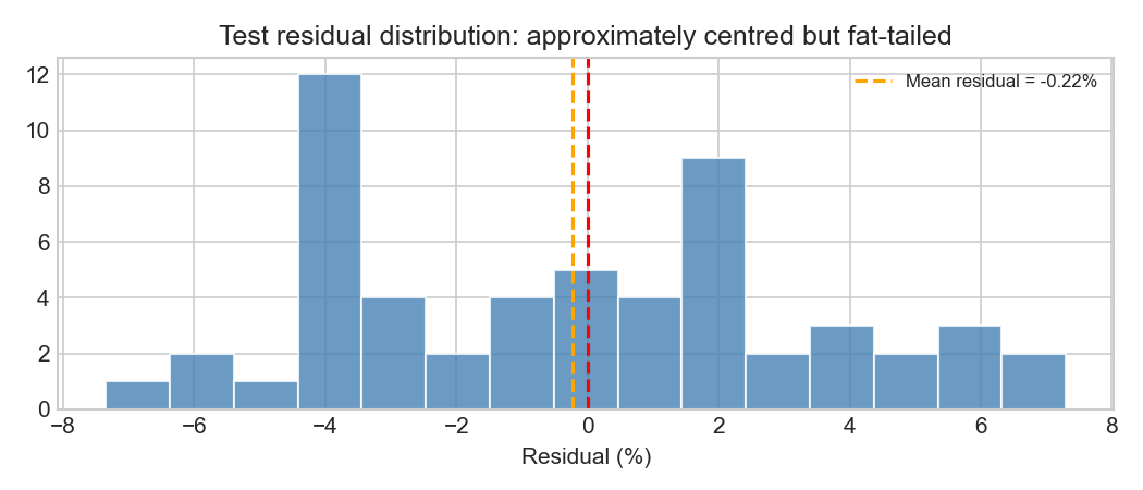
ax.set_title("Test residual distribution: approximately centred but fat-tailed")
ax.set_xlabel("Residual (%)")
ax.legend(fontsize=8)
plt.tight_layout()
plt.savefig("w08-residuals-dist-baseline.png", dpi=150)
plt.show()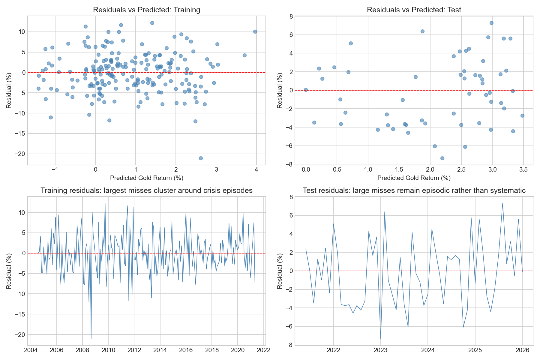

Residuals fluctuate around zero in both the training and test samples, suggesting that the model does not exhibit strong systematic bias overall. The residual-versus-predicted plots also do not show a strong remaining linear pattern, which is reassuring: the model captures some broad macro-financial structure, even though a substantial share of return variation remains unexplained.

The table of largest residuals shows that the biggest misses are concentrated in identifiable historical episodes rather than scattered randomly across time. In the training sample, the most extreme errors occur in July–September 2008, October 2009, July–December 2011, and May 2013. These periods correspond to the Global Financial Crisis, its aftermath, the Eurozone sovereign-debt turmoil, and the 2013 taper-period market dislocation. In such episodes, gold moved abruptly because of crisis dynamics, safe-haven flows, and rapid repricing in inflation and risk expectations, forces that a linear macro-financial model can only capture imperfectly.

In the test sample, the average residual is close to zero (around −0.22 percentage points), so there is little evidence of a strong overall tendency to over-predict or under-predict returns across the holdout period as a whole. The largest misses are instead episodic. The biggest residuals occur in January–February 2023, August 2023, October 2024, and several months in 2025. This suggests that the model performs reasonably on average but still struggles during months dominated by abrupt repricing, geopolitical uncertainty, or sharp shifts in safe-haven demand.

The residual distribution is centred close to zero but exhibits fat tails, meaning that large forecast errors occur more frequently than would be expected under a normal distribution. This is characteristic of financial return data and reflects the importance of occasional large market shocks. Overall, the residual diagnostics suggest that the model is reasonably well calibrated on average, but still struggles with the shock-driven and episodic nature of gold returns.

1.5.4 Improving the baseline model

The baseline OLS model outperformed the naïve historical-mean forecast on the final holdout test set, but its predictive power remained limited. It achieved a positive test $R^2$ of 0.138, reduced MAE from 3.37% to 3.05%, and reduced RMSE from 3.99% to 3.57%. These are encouraging results, but they do not imply that the model is strong in an absolute sense: a typical forecast error of around 3 percentage points remains large relative to the scale of monthly gold returns.

The earlier diagnostics also showed that the baseline model’s largest misses occur during episodic shock periods, such as the Global Financial Crisis, the Eurozone stress period, and several months in 2023–2025. This suggests that the main weakness of the linear baseline is not strong average bias, but difficulty in dealing with regime shifts, delayed macro transmission, and abrupt non-linear repricing.

On that basis, three extensions are worth testing:

Time-aware cross-validation to assess whether the apparent baseline signal is stable across historical subperiods
Lagged predictors to test whether macro-financial effects transmit with delay
A non-linear tree-based model (LightGBM) to test whether threshold effects and interactions improve forecasting accuracy

The aim is not simply to search for a slightly higher $R^2$, but to determine whether a richer model can improve forecasting consistently across multiple metrics and in a way that remains economically meaningful.

Step 1: Time-Aware cross-validation on the baseline

Before modifying the model, we evaluate the baseline OLS specification using expanding-window cross-validation within the training sample.

Why TimeSeriesSplit rather than random k-fold? In a time series, future observations must never be used to predict the past. Random k-fold cross-validation would mix different time periods and introduce look-ahead bias. TimeSeriesSplit respects chronology by ensuring that each validation window comes strictly after its training window.

Why this matters here: the sample spans several very different regimes, i.e the post-dot-com period, the Global Financial Crisis, the Eurozone crisis, the post-2013 adjustment, and the inflation/geopolitical environment of the 2020s. A model that performs well in one train/test split may simply be benefitting from a favourable historical window.

To keep the evaluation consistent with the holdout analysis, we compute $R^2$, MAE, and RMSE in each fold.

tscv = TimeSeriesSplit(n_splits=5)

def cv_evaluate_ols(X, y, splitter):
    r2_scores, mae_scores, rmse_scores = [], [], []

    for idx_tr, idx_val in splitter.split(X):
        model = LinearRegression()
        model.fit(X.iloc[idx_tr], y.iloc[idx_tr])

        y_val_true = y.iloc[idx_val]
        y_val_pred = model.predict(X.iloc[idx_val])

        r2_scores.append(r2_score(y_val_true, y_val_pred))
        mae_scores.append(mean_absolute_error(y_val_true, y_val_pred))
        rmse_scores.append(np.sqrt(mean_squared_error(y_val_true, y_val_pred)))

    return r2_scores, mae_scores, rmse_scores

cv_baseline_r2, cv_baseline_mae, cv_baseline_rmse = cv_evaluate_ols(X_train, y_train, tscv)

print(f"Baseline OLS — CV R² per fold: {[round(s,4) for s in cv_baseline_r2]}")
print(f"Baseline OLS — CV MAE per fold: {[round(s,4) for s in cv_baseline_mae]}")
print(f"Baseline OLS — CV RMSE per fold: {[round(s,4) for s in cv_baseline_rmse]}")
print(f"Mean CV R²: {np.mean(cv_baseline_r2):.4f} ± {np.std(cv_baseline_r2):.4f}")
print(f"Mean CV MAE: {np.mean(cv_baseline_mae):.4f}% ± {np.std(cv_baseline_mae):.4f}")
print(f"Mean CV RMSE: {np.mean(cv_baseline_rmse):.4f}% ± {np.std(cv_baseline_rmse):.4f}")

Baseline OLS — CV R² per fold: [-26.7551, -0.5363, -0.2154, -0.1248, -0.7991]
Baseline OLS — CV MAE per fold: [26.6544, 5.7512, 4.3148, 3.1111, 4.2859]
Baseline OLS — CV RMSE per fold: [34.9858, 6.7938, 5.2032, 4.0605, 5.5343]
Mean CV R²: -5.6861 ± 10.5372
Mean CV MAE: 8.8234% ± 8.9547
Mean CV RMSE: 11.3155% ± 11.8670

To understand where this instability comes from, we inspect the date ranges of the folds.

def inspect_tscv_folds(X, y, dates, splitter, model_class=LinearRegression, model_kwargs=None):
    if model_kwargs is None:
        model_kwargs = {}

    fold_info = []

    for fold, (idx_tr, idx_val) in enumerate(splitter.split(X), start=1):
        model = model_class(**model_kwargs)
        model.fit(X.iloc[idx_tr], y.iloc[idx_tr])
        y_val_pred = model.predict(X.iloc[idx_val])
        y_val_true = y.iloc[idx_val]
        val_dates = dates.iloc[idx_val]

        fold_info.append({
            "fold": fold,
            "train_start": dates.iloc[idx_tr].min(),
            "train_end": dates.iloc[idx_tr].max(),
            "val_start": val_dates.min(),
            "val_end": val_dates.max(),
            "r2": r2_score(y_val_true, y_val_pred),
            "mae": mean_absolute_error(y_val_true, y_val_pred),
            "rmse": np.sqrt(mean_squared_error(y_val_true, y_val_pred))
        })

    return pd.DataFrame(fold_info)

baseline_fold_df = inspect_tscv_folds(
    X_train,
    y_train,
    train.loc[train_clean.index, "date"].reset_index(drop=True),
    tscv
)

print(baseline_fold_df.to_string(index=False))

 fold train_start  train_end  val_start    val_end         r2       mae      rmse
    1  2004-08-01 2007-08-01 2007-09-01 2010-05-01 -26.755052 26.654353 34.985844
    2  2004-08-01 2010-05-01 2010-06-01 2013-02-01  -0.536315  5.751158  6.793764
    3  2004-08-01 2013-02-01 2013-03-01 2015-11-01  -0.215379  4.314753  5.203226
    4  2004-08-01 2015-11-01 2015-12-01 2018-08-01  -0.124761  3.111065  4.060525
    5  2004-08-01 2018-08-01 2018-09-01 2021-05-01  -0.799089  4.285863  5.534280

These cross-validation results are much weaker than the single holdout test result. The mean CV $R^2$ is strongly negative, and the fold-to-fold variation is extremely large. The most striking case is Fold 1, whose validation window runs from September 2007 to May 2010. That period covers the onset of the Global Financial Crisis and its immediate aftermath. The model is trained only on pre-crisis data and then evaluated in a radically different regime characterised by extreme stress, collapsing inflation expectations, emergency monetary easing, and unusually large gold moves. The very poor fold performance therefore reflects a genuine regime break, not merely ordinary forecast noise.

Later folds are less catastrophic but still weak. Fold 2 covers June 2010 to February 2013, a period overlapping with Eurozone sovereign-debt stress and elevated safe-haven demand, while Fold 5 covers September 2018 to May 2021, spanning the COVID shock and its aftermath. Together, these results suggest that the macro-financial relationship captured by the baseline model is fragile and time-varying. The positive holdout result remains encouraging, but it should be interpreted as period-specific rather than universally stable.

Step 2: Linear regression with lagged features

The baseline model already uses predictors observed in month $t$ to forecast the gold return in month $t+1$. Adding lags therefore tests a more specific question:

Do macro-financial conditions from month $t-1$ contain useful information for forecasting returns at month $t+1$, beyond the information already present at month $t$?

This is plausible for both economic and empirical reasons.

From an economic perspective, some channels may operate with delay:

tighter financial conditions may influence portfolio allocation gradually rather than instantly
inflationary pressure may feed through to gold demand over more than one month
shifts in global sentiment may diffuse across markets with a lag

From an empirical perspective, the baseline residuals suggest that the model sometimes captures the right broad macro backdrop, but misses the timing of gold’s response. Lagged variables therefore test whether part of the baseline weakness reflects delayed transmission rather than complete absence of signal.

We augment the baseline feature set with one-month lags of each predictor.

for f in features:
    modelling_df[f + "_lag1"] = modelling_df[f].shift(1)

features_lagged = features + [f + "_lag1" for f in features]

train_lag = modelling_df.iloc[:split_idx].copy()
test_lag  = modelling_df.iloc[split_idx:].copy()

train_lag = train_lag[["date"] + features_lagged + ["target"]].dropna()
test_lag  = test_lag[["date"] + features_lagged + ["target"]].dropna()

X_train_lag = train_lag[features_lagged]
y_train_lag = train_lag["target"]
X_test_lag  = test_lag[features_lagged]
y_test_lag  = test_lag["target"]

print(f"Lagged model training: {len(X_train_lag)} obs, {len(features_lagged)} features")
print(f"Obs-to-predictor ratio: {len(X_train_lag) / len(features_lagged):.1f}:1")

Lagged model training: 201 obs, 10 features
Obs-to-predictor ratio: 20.1:1

The first observation is lost mechanically because lagged values are unavailable for the first month. This is deterministic missingness, not a data-quality problem, and is handled appropriately by dropna().

lr_lag = LinearRegression()
lr_lag.fit(X_train_lag, y_train_lag)

evaluate(y_train_lag, lr_lag.predict(X_train_lag), "Lagged Train")
evaluate(y_test_lag,  lr_lag.predict(X_test_lag),  "Lagged Test ")

Lagged Train: R²=0.0837, MAE=3.8229%, RMSE=4.8257%
Lagged Test : R²=-0.1353, MAE=3.3143%, RMSE=4.0970%

The lagged model improves in-sample fit slightly relative to the baseline, but performs materially worse out of sample. On the holdout test set, its $R^2$ turns negative, its MAE rises from 3.05% to 3.31%, and its RMSE rises from 3.57% to 4.10%. This is strong evidence that the additional lagged predictors are adding noise rather than useful predictive information at the one-month horizon.

We confirm this with expanding-window CV.

cv_lagged_r2, cv_lagged_mae, cv_lagged_rmse = cv_evaluate_ols(X_train_lag, y_train_lag, tscv)

print(f"Lagged OLS — CV R² per fold: {[round(s,4) for s in cv_lagged_r2]}")
print(f"Lagged OLS — CV MAE per fold: {[round(s,4) for s in cv_lagged_mae]}")
print(f"Lagged OLS — CV RMSE per fold: {[round(s,4) for s in cv_lagged_rmse]}")
print(f"Mean CV R²: {np.mean(cv_lagged_r2):.4f} ± {np.std(cv_lagged_r2):.4f}")
print(f"Mean CV MAE: {np.mean(cv_lagged_mae):.4f}% ± {np.std(cv_lagged_mae):.4f}")
print(f"Mean CV RMSE: {np.mean(cv_lagged_rmse):.4f}% ± {np.std(cv_lagged_rmse):.4f}")

Lagged OLS — CV R² per fold: [-7.9355, -0.2412, -0.2180, -0.2637, -0.7112]
Lagged OLS — CV MAE per fold: [13.8367, 4.6891, 4.3878, 3.3197, 4.1642]
Lagged OLS — CV RMSE per fold: [19.8509, 6.1064, 5.2089, 4.3041, 5.3974]
Mean CV R²: -1.8739 ± 3.0363
Mean CV MAE: 6.0795% ± 3.9052
Mean CV RMSE: 8.1735% ± 5.8669

The cross-validation results reinforce the holdout evidence that the lagged specification is not an improvement. Its average CV performance is less extreme than the baseline OLS because it does not suffer the same catastrophic collapse in the first crisis-period fold, but that should not be confused with genuine superiority. On the final holdout test set, the lagged model is clearly worse than the contemporaneous baseline on all three metrics: its $R^2$ turns negative, and both MAE and RMSE increase. In other words, adding lagged predictors makes the model slightly better at fitting the training data, but not better at generalising to new periods. Economically, this suggests that whatever useful macro-financial signal exists at the one-month horizon is either already contained in contemporaneous variables or is too weak and unstable to be recovered reliably through simple one-month lags.

Step 3: A non-Linear alternative (LightGBM)

The baseline residual diagnostics suggest a second possible limitation of OLS: the model is too conservative, with predictions compressed into a narrow band and the largest misses concentrated in shock periods. That pattern is consistent with the idea that gold may react to macro-financial conditions in a non-linear way.

For example:

safe-haven demand may intensify only once financial stress crosses a threshold
supply-chain stress may matter more when inflation anxiety is already elevated
the interaction between global market conditions and real yields may matter more than either variable alone

A gradient-boosted tree model can, in principle, capture such threshold effects and interactions without requiring them to be specified manually.

We use LightGBM because it is well suited to small tabular datasets, can model non-linearities and interactions, and includes built-in regularisation controls that matter in a short sample spanning multiple regimes.

Why RandomizedSearchCV? The hyperparameter space for boosting models is multi-dimensional. Exhaustive grid search would be more costly without offering much added value in a dataset of this size. RandomizedSearchCV provides a pragmatic compromise: it explores a broad range of configurations efficiently and is usually sufficient to identify a well-regularised region of the parameter space.

Why optimise LightGBM using RMSE? In this setting, RMSE is the most sensible tuning objective. The economically most important failures in gold forecasting occur during periods of financial stress and crisis, precisely when forecast errors tend to be largest. RMSE penalises these large misses more heavily than MAE and is therefore better aligned with the practical objective of reducing the most consequential forecast errors. It also matches the earlier residual analysis, which showed that the baseline model’s weakness is concentrated in large episodic misses rather than small average deviations. In practice, optimising on $R^2$, MAE, or RMSE led to the same best hyperparameters, so the choice does not materially affect the final result; RMSE is retained because it is the most economically meaningful criterion here.

param_grid = {
    "num_leaves": [15, 31, 50],
    "max_depth": [3, 5, 7],
    "learning_rate": [0.01, 0.05, 0.1],
    "n_estimators": [50, 100, 200],
    "subsample": [0.7, 0.8, 1.0],
    "colsample_bytree": [0.7, 0.8, 1.0]
}

lgbm = lgb.LGBMRegressor(random_state=42, verbose=-1)

search = RandomizedSearchCV(
    estimator=lgbm,
    param_distributions=param_grid,
    n_iter=30,
    cv=tscv,
    scoring="neg_mean_squared_error",
    n_jobs=2,
    random_state=42,
    refit=True,
    pre_dispatch="2*n_jobs"
)

search.fit(X_train, y_train)
best_lgbm = search.best_estimator_

print(f"Best parameters: {search.best_params_}")

Best parameters: {'subsample': 1.0, 'num_leaves': 15, 'n_estimators': 100, 'max_depth': 3, 'learning_rate': 0.01, 'colsample_bytree': 0.8}

The selected LightGBM model is shallow and heavily regularised: small trees, low learning rate, and moderate feature subsampling. That is informative in itself. If the dataset contained strong exploitable non-linearity, the optimal configuration might tolerate more complexity. Instead, the search favours a restrained specification, suggesting that the underlying signal is weak and that richer trees would overfit quickly.

To evaluate the tuned model consistently, we compute fold-by-fold CV metrics using the selected configuration.

fold_metrics = []

for i, (idx_tr, idx_val) in enumerate(tscv.split(X_train, y_train), start=1):
    X_tr, X_val = X_train.iloc[idx_tr], X_train.iloc[idx_val]
    y_tr, y_val = y_train.iloc[idx_tr], y_train.iloc[idx_val]

    model_fold = lgb.LGBMRegressor(
        **search.best_params_,
        random_state=42,
        verbose=-1
    )
    model_fold.fit(X_tr, y_tr)
    y_val_pred = model_fold.predict(X_val)

    fold_metrics.append({
        "fold": i,
        "rmse": np.sqrt(mean_squared_error(y_val, y_val_pred)),
        "mae": mean_absolute_error(y_val, y_val_pred),
        "r2": r2_score(y_val, y_val_pred)
    })

metrics_df = pd.DataFrame(fold_metrics)
print(metrics_df.to_string(index=False))

fold     rmse      mae        r2
    1 6.641044 5.112349 -0.000069
    2 5.585200 4.440913 -0.038333
    3 5.192616 4.257051 -0.210428
    4 3.840760 3.143320 -0.006306
    5 4.390086 3.525296 -0.132078

We can summarise these fold-level metrics directly.

summary_table = pd.DataFrame({
    "Metric": ["RMSE", "MAE", "R²"],
    "Mean": [
        metrics_df["rmse"].mean(),
        metrics_df["mae"].mean(),
        metrics_df["r2"].mean()
    ],
    "Std": [
        metrics_df["rmse"].std(),
        metrics_df["mae"].std(),
        metrics_df["r2"].std()
    ],
    "Min": [
        metrics_df["rmse"].min(),
        metrics_df["mae"].min(),
        metrics_df["r2"].min()
    ],
    "Max": [
        metrics_df["rmse"].max(),
        metrics_df["mae"].max(),
        metrics_df["r2"].max()
    ]
}).round(4)

print(summary_table.to_markdown(index=False))

| Metric   |   Mean |   Std |    Min |    Max |
|:---------|-------:|------:|-------:|-------:|
| RMSE     | 5.1299 | 1.0844| 3.8408 | 6.6410 |
| MAE      | 4.0958 | 0.7764| 3.1433 | 5.1123 |
| R²       | -0.0774| 0.0912| -0.2104| -0.0001|

This summary is more informative than a single mean CV score. It shows that:

RMSE averages about 5.13 percentage points, with meaningful but not enormous dispersion across folds
MAE averages about 4.10 percentage points
R² remains negative in every fold, but varies within a much narrower band than baseline OLS

So LightGBM improves stability relative to OLS, but not enough to produce positive average explanatory power in rolling-origin validation.

The fold-level RMSE plot makes this clearer.

best_fold_rmse = metrics_df["rmse"].tolist()

plt.figure(figsize=(10, 5))
plt.plot(range(1, len(best_fold_rmse) + 1), best_fold_rmse,
         marker="o", linestyle="-", color="steelblue", linewidth=2,
         label="Best config RMSE per fold")

plt.axhline(y=np.mean(best_fold_rmse), color="green", linestyle="--",
            label=f"Mean RMSE: {np.mean(best_fold_rmse):.4f}")

plt.fill_between(
    range(1, len(best_fold_rmse) + 1),
    np.mean(best_fold_rmse) - np.std(best_fold_rmse),
    np.mean(best_fold_rmse) + np.std(best_fold_rmse),
    color="green", alpha=0.2, label="±1 SD"
)

plt.xlabel("Time Series CV Fold")
plt.ylabel("RMSE")
plt.title("Best LightGBM Model (RMSE-Optimised): Performance Across CV Folds")
plt.legend()
plt.grid(alpha=0.3, axis="y")
plt.tight_layout()
plt.show()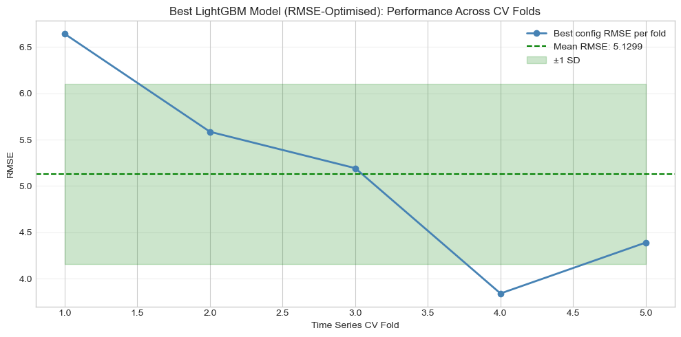

This plot confirms that the model still struggles most in the earliest fold, but the fold-to-fold variation is much less dramatic than under baseline OLS. In that sense, LightGBM appears more robust across regimes, even though it does not ultimately outperform the baseline on the final holdout test set.

We now evaluate the tuned model on the train and test samples.

evaluate(y_train, best_lgbm.predict(X_train), "LightGBM Train")
evaluate(y_test,  best_lgbm.predict(X_test),  "LightGBM Test ")

LightGBM Train: R²=0.1161, MAE=3.7067%, RMSE=4.7283%
LightGBM Test : R²=-0.0544, MAE=3.3503%, RMSE=3.9484%

LightGBM achieves the strongest in-sample fit of the three models considered, but this does not translate into superior holdout performance. Its test $R^2$ is negative, and both MAE and RMSE are worse than the baseline OLS. Relative to the lagged OLS model, however, LightGBM is somewhat better: it has a less negative test $R^2$, lower test RMSE, and much greater stability across CV folds. So the non-linear model does not uncover a strong new signal, but it does appear more robust than simply adding linear lags.

SHAP interpretation across models

To make interpretability more comparable across model classes, we supplement the coefficient table and tree-based feature importance with SHAP summary plots for all three specifications. SHAP decomposes predictions into feature-level contributions and therefore provides a common language for comparing linear and non-linear models.

Baseline OLS SHAP

explainer_ols = shap.LinearExplainer(lr, X_train)
shap_values_ols = explainer_ols.shap_values(X_test)

plt.figure()
shap.summary_plot(shap_values_ols, X_test, feature_names=X_test.columns, show=False)
plt.title("Baseline OLS model")
plt.tight_layout()
plt.show()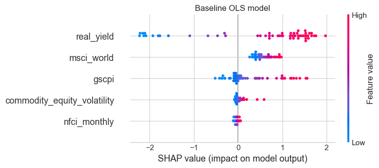

Lagged OLS SHAP

explainer_lag = shap.LinearExplainer(lr_lag, X_train_lag)
shap_values_lag = explainer_lag.shap_values(X_test_lag)

plt.figure()
shap.summary_plot(shap_values_lag, X_test_lag, feature_names=X_test_lag.columns, show=False)
plt.title("Lagged OLS model")
plt.tight_layout()
plt.show()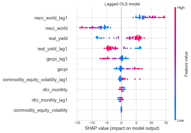

LightGBM SHAP

explainer_lgb = shap.TreeExplainer(best_lgbm)
shap_values_lgb = explainer_lgb.shap_values(X_test)

plt.figure()
shap.summary_plot(shap_values_lgb, X_test, feature_names=X_test.columns, show=False)
plt.title("LightGBM")
plt.tight_layout()
plt.show()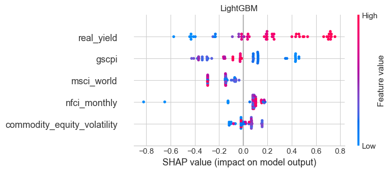

The SHAP plots do more than rank variables by importance: they also show the direction in which high or low values of each predictor push the model’s forecast.

In the baseline OLS model, high values of real_yield contribute positively to predicted next-month gold returns, while low values contribute negatively. This reproduces the positive coefficient seen earlier, but SHAP makes the pattern more visual: periods of relatively high real yields in this sample are associated with higher predicted gold returns, not lower. Economically, this reinforces the earlier caution that real_yield is not behaving here as a clean opportunity-cost variable in the textbook sense. Instead, it seems to be acting partly as a regime indicator, picking up episodes in which elevated real yields coincide with stressed macro-financial conditions or post-shock adjustment periods in which gold subsequently performed strongly.

For gscpi, higher values generally push predictions upward and lower values push them downward. This is economically sensible: elevated global supply-chain pressure signals an environment of inflationary strain and macro uncertainty, both of which can support gold demand as a real asset and inflation-sensitive store of value.

For msci_world, the contribution is positive when the index is high and negative when it is low, although the magnitude is smaller than for real_yield. This suggests that stronger global equity conditions are associated, at the margin, with somewhat higher predicted gold returns in this specification. That is not the simplest “gold as pure risk-off asset” story, but it is plausible in a sample where gold sometimes rose alongside broader market strength during liquidity-rich or recovery periods. In other words, msci_world seems to be capturing part of the broader global macro regime, not a simple safe-haven inverse relation.

nfci_monthly has relatively small SHAP values in the baseline model, but the direction is still broadly interpretable: tighter financial conditions tend to push forecasts upward slightly, while looser conditions pull them downward. This is consistent with the safe-haven channel, though its incremental effect is modest once the other predictors are already in the model.

commodity_equity_volatility contributes very little in either direction. Its SHAP spread is narrow, which confirms what the coefficient table already suggested: this variable adds only limited extra predictive content once the main macro-financial channels are accounted for.

In the lagged OLS model, the SHAP plot shows that the model actively uses both contemporaneous and lagged versions of real_yield, msci_world, and gscpi. High values of msci_world_lag1 and contemporaneous real_yield tend to push predictions upward, while high values of contemporaneous msci_world and real_yield_lag1 more often push them downward. Economically, this suggests that once lagged variables are introduced, the model starts fitting a more complicated timing structure in which current and lagged versions of similar macro signals pull in opposite directions. That is exactly the kind of pattern that can improve in-sample fit while worsening out-of-sample generalisation: the model is finding timing relationships in the training data, but those relationships are not stable enough to survive holdout evaluation.

In LightGBM, real_yield again dominates, and high values mostly push predictions upward while low values tend to pull them downward. That consistency across linear and non-linear models strengthens the conclusion that the positive real_yield signal is real in the sample, even if its economic interpretation remains counterintuitive.

For gscpi, the LightGBM SHAP plot is more nuanced than in OLS. The contribution pattern is not purely linear: different parts of the gscpi distribution contribute differently, which suggests that supply-chain stress may matter in a state-dependent way rather than through a single constant slope. That is economically plausible: moderate supply-chain pressure and extreme supply-chain disruption may have different implications for inflation expectations, safe-haven demand, and gold’s role in portfolios.

msci_world contributes less strongly than in the linear models, and its SHAP values are centred closer to zero. This suggests that in the non-linear model, global equity conditions matter, but mostly as part of interactions with other predictors rather than as a strong standalone driver.

nfci_monthly also shows a more clearly directional positive contribution in LightGBM than in baseline OLS: tighter financial conditions tend to push predictions upward, consistent with gold’s safe-haven role. Finally, commodity_equity_volatility remains weak across all three models, indicating that this channel adds relatively little stable signal at the monthly horizon.

Overall, the SHAP evidence is consistent across models in one important sense: the same core variables, especially real_yield, gscpi, msci_world, and nfci_monthly, keep reappearing as the main drivers. The issue is not that different models identify completely different signals; rather, they all identify a similar weak signal, which remains difficult to exploit robustly out of sample.

Diagnostic comparison across models

To compare the models more directly, we generate the same predicted-versus-actual and residual-over-time diagnostics for each specification.

def diagnostic_plots(results_df, model_name):
    fig, axes = plt.subplots(2, 2, figsize=(12, 8))

    train_df = results_df[results_df["split"] == "train"]
    test_df = results_df[results_df["split"] == "test"]

    for ax, df, title in [
        (axes[0, 0], train_df, f"{model_name}: Predicted vs Actual (Training)"),
        (axes[0, 1], test_df,  f"{model_name}: Predicted vs Actual (Test)")
    ]:
        ax.scatter(df["y_pred"], df["y_true"], alpha=0.7)
        min_val = min(df["y_true"].min(), df["y_pred"].min())
        max_val = max(df["y_true"].max(), df["y_pred"].max())
        ax.plot([min_val, max_val], [min_val, max_val], linestyle="--", color="red")
        ax.set_xlabel("Predicted Return (%)")
        ax.set_ylabel("Actual Return (%)")
        ax.set_title(title)

    axes[1, 0].plot(train_df["date"], train_df["residual"], linewidth=0.8)
    axes[1, 0].axhline(0, color="red", linestyle="--", linewidth=0.9)
    axes[1, 0].set_title(f"{model_name}: Training residuals")
    axes[1, 0].set_ylabel("Residual (%)")

    axes[1, 1].plot(test_df["date"], test_df["residual"], linewidth=0.8)
    axes[1, 1].axhline(0, color="red", linestyle="--", linewidth=0.9)
    axes[1, 1].set_title(f"{model_name}: Test residuals")
    axes[1, 1].set_ylabel("Residual (%)")

    plt.tight_layout()
    plt.show()

Baseline OLS diagnostics

baseline_train_results = pd.DataFrame({
    "date": train.loc[train_clean.index, "date"].values,
    "y_true": y_train.values,
    "y_pred": y_pred_train,
    "split": "train"
})
baseline_train_results["residual"] = baseline_train_results["y_true"] - baseline_train_results["y_pred"]

baseline_test_results = pd.DataFrame({
    "date": test.loc[test_clean.index, "date"].values,
    "y_true": y_test.values,
    "y_pred": y_pred_test,
    "split": "test"
})
baseline_test_results["residual"] = baseline_test_results["y_true"] - baseline_test_results["y_pred"]

baseline_results = pd.concat([baseline_train_results, baseline_test_results], ignore_index=True)
diagnostic_plots(baseline_results, "OLS baseline")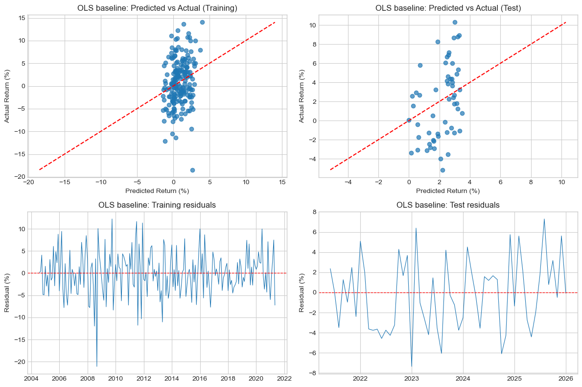

Lagged OLS diagnostics

lag_train_pred = lr_lag.predict(X_train_lag)
lag_test_pred = lr_lag.predict(X_test_lag)

lag_train_results = pd.DataFrame({
    "date": train_lag["date"].values,
    "y_true": y_train_lag.values,
    "y_pred": lag_train_pred,
    "split": "train"
})
lag_train_results["residual"] = lag_train_results["y_true"] - lag_train_results["y_pred"]

lag_test_results = pd.DataFrame({
    "date": test_lag["date"].values,
    "y_true": y_test_lag.values,
    "y_pred": lag_test_pred,
    "split": "test"
})
lag_test_results["residual"] = lag_test_results["y_true"] - lag_test_results["y_pred"]

lag_results = pd.concat([lag_train_results, lag_test_results], ignore_index=True)
diagnostic_plots(lag_results, "OLS + lags")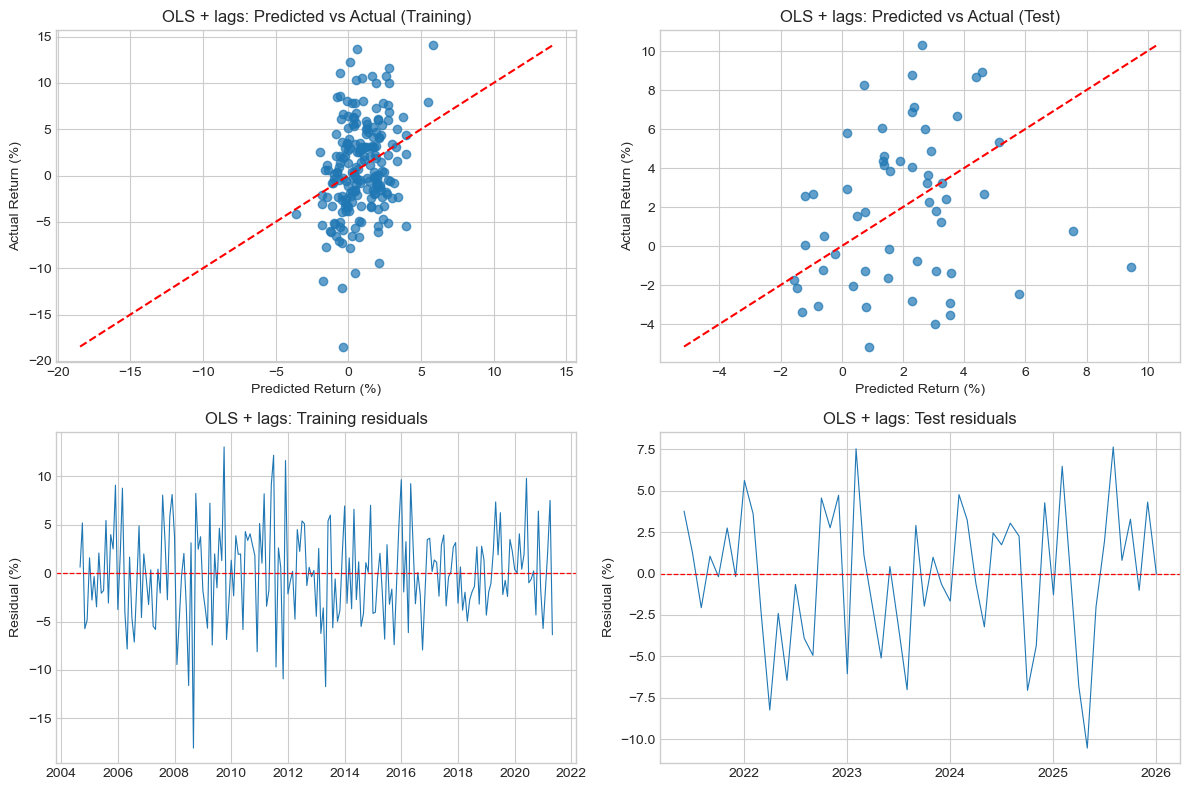

LightGBM diagnostics

lgb_train_pred = best_lgbm.predict(X_train)
lgb_test_pred = best_lgbm.predict(X_test)

lgb_train_results = pd.DataFrame({
    "date": train.loc[train_clean.index, "date"].values,
    "y_true": y_train.values,
    "y_pred": lgb_train_pred,
    "split": "train"
})
lgb_train_results["residual"] = lgb_train_results["y_true"] - lgb_train_results["y_pred"]

lgb_test_results = pd.DataFrame({
    "date": test.loc[test_clean.index, "date"].values,
    "y_true": y_test.values,
    "y_pred": lgb_test_pred,
    "split": "test"
})
lgb_test_results["residual"] = lgb_test_results["y_true"] - lgb_test_results["y_pred"]

lgb_results = pd.concat([lgb_train_results, lgb_test_results], ignore_index=True)
diagnostic_plots(lgb_results, "LightGBM")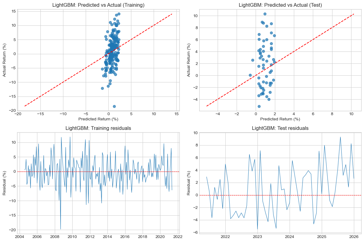

These plots show three important patterns.

First, all three models predict within a much narrower range than realised gold returns, confirming that large market moves remain inherently difficult to forecast from macro-financial variables alone.

Second, the lagged OLS model produces a somewhat broader prediction range than baseline OLS, but this does not improve alignment with realised returns. Instead, the test scatter becomes more diffuse around the 45-degree line and residual swings become larger, especially in 2023–2025. This is consistent with the worse test RMSE and negative test $R^2$.

Third, LightGBM is more conservative. Its test predictions are compressed into a relatively narrow band, and while this improves fold-to-fold stability in cross-validation, it does not reduce the large episodic misses enough to outperform the baseline on the final holdout window.

Overall, the diagnostics reinforce the metric-based comparison: neither extension resolves the baseline model’s main weakness, namely the inability to anticipate the largest, shock-driven moves in gold returns.

Model comparison

Bringing all results together:

Model	Train R²	Mean CV R²	Mean CV MAE	Mean CV RMSE	Test R²	Test MAE	Test RMSE
Naïve (historical mean)	—	—	—	—	−0.077	3.37%	3.99%
OLS baseline	0.049	−5.686	8.82%	11.32%	+0.138	3.05%	3.57%
OLS + lags	0.084	−1.874	6.08%	8.17%	−0.135	3.31%	4.10%
LightGBM	0.116	−0.077	4.10%	5.13%	−0.054	3.35%	3.95%

A visual comparison is also useful.

comparison_df = pd.DataFrame({
    "Model": ["Naive", "OLS baseline", "OLS + lags", "LightGBM"],
    "Test_R2": [-0.0772, 0.1383, -0.1353, -0.0544],
    "Test_MAE": [3.3659, 3.0510, 3.3143, 3.3503],
    "Test_RMSE": [3.9908, 3.5693, 4.0970, 3.9484]
})

fig, axes = plt.subplots(1, 3, figsize=(12, 3.5))

for ax, metric in zip(axes, ["Test_R2", "Test_MAE", "Test_RMSE"]):
    ax.bar(comparison_df["Model"], comparison_df[metric])
    ax.set_title(metric.replace("_", " "))
    ax.tick_params(axis="x", rotation=30)

plt.tight_layout()
plt.show()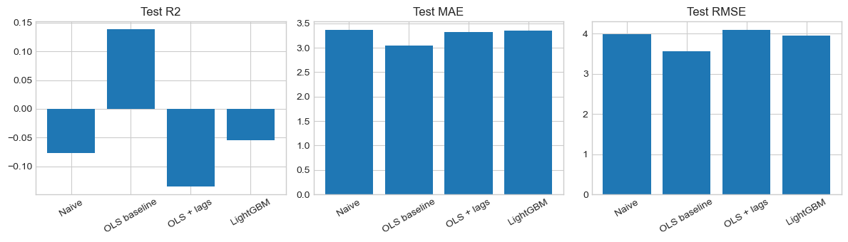

These results should be interpreted jointly across train fit, cross-validation stability, and holdout test performance, rather than on the holdout test alone.

The baseline OLS has the strongest final holdout performance by a clear margin: it has the highest test $R^2$, the lowest test MAE, and the lowest test RMSE. However, it also has by far the weakest cross-validation profile. Its CV performance is extremely unstable across folds, with one catastrophic early fold and very large train–CV discrepancies. This means that its good test result should not be read as evidence of a uniformly stable forecasting relationship. Instead, it suggests that the model performs well in the particular final test window, but generalises poorly across some earlier regimes.

The lagged OLS modestly improves train fit relative to the baseline, but that gain does not survive out-of-sample evaluation. Its train–test gap is large, its test $R^2$ turns negative, and its test RMSE is the worst of the three estimated models. On balance, this is the clearest case of additional complexity failing to generalise. The lagged model is fitting timing patterns in the training data that do not persist.

The LightGBM model has the strongest in-sample fit and the best cross-validation profile of the three estimated models. Its mean CV $R^2$, CV MAE, and CV RMSE are all much better than those of baseline OLS, and its fold-to-fold variation is far smaller. In other words, it is the most stable across rolling subperiods. However, that greater stability does not translate into the strongest final holdout result: its test performance remains worse than the baseline OLS across all three test metrics, although it is still slightly better than the naïve benchmark and clearly better than the lagged OLS on RMSE.

The model choice depends on what is prioritised.

If the sole priority is best performance on the final holdout window, then the baseline OLS is preferred: it has the highest test $R^2$, the lowest test MAE, and the lowest test RMSE. It is also the easiest model to interpret economically.

However, if the priority is more stable performance across time, with fewer catastrophic failures when the historical regime changes, then LightGBM is the more robust choice. Its cross-validation results are far more stable than those of the baseline OLS, and its fold-level errors remain within a much narrower range. By contrast, the OLS model performs very well in the final holdout period but breaks down dramatically in earlier validation windows, especially when asked to extrapolate from pre-crisis data into the Global Financial Crisis. That makes its apparent success look strongly window-dependent.

On balance, I would therefore treat the baseline OLS as the most interpretable benchmark, but favour LightGBM as the model I would trust more for practical forecasting. The trade-off is essentially one of accuracy versus stability: OLS delivers the strongest result in one particular test period, whereas LightGBM behaves more consistently across different historical windows and avoids the extreme failures seen in the linear model. In a macro-financial setting characterised by regime shifts, that robustness is an important advantage.

The most defensible overall conclusion is therefore not that one model dominates on every criterion, but that they serve different purposes: OLS is the clearest model for economic interpretation, while LightGBM is the more stable forecasting specification across regimes.

1.6 Discussion

How predictable are gold returns in this sample?

The evidence in this exercise suggests that monthly gold returns are only weakly predictable from macro-financial data, and that whatever predictability exists is regime-dependent rather than stable.

The most favourable result comes from the baseline OLS model on the final holdout test set. It achieves a test $R^2$ of 0.138, reduces MAE from 3.37% under the naïve historical-mean forecast to 3.05%, and reduces RMSE from 3.99% to 3.57%. These results show that the selected predictors contain some genuine out-of-sample signal: the model beats the mean forecast across all three holdout metrics.

At the same time, the magnitude of that signal is limited. A test MAE of 3.05 percentage points is still large relative to the size of typical monthly gold returns, and the predicted values remain compressed into a much narrower range than the realised returns. The predicted-versus-actual plots show that all models struggle to reproduce the largest positive and negative monthly moves. The residual analysis reinforces this: the biggest misses are concentrated in months such as September 2008, October 2009, mid/late 2011, and several months in 2023–2025, all periods dominated by crisis dynamics, abrupt repricing, or unusually strong safe-haven demand.

Cross-validation makes the predictability question look even weaker. For the baseline OLS, the mean CV $R^2$ is −5.686, with a huge standard deviation of 10.537, and the first fold — validating on September 2007 to May 2010 — is catastrophically poor. This tells us that the baseline signal is not stable across historical windows. The relationship between macro variables and gold returns appears to change materially across regimes, especially during crisis periods.

The lagged OLS and LightGBM extensions do not overturn this conclusion. The lagged model performs worse than the baseline on the final test set, with test $R^2 = -0.135$ and RMSE = 4.10%, and it also performs poorly in cross-validation. LightGBM is more stable across CV folds, with mean CV $R^2 = -0.077$ and mean CV RMSE = 5.13%, but it still does not beat the baseline in the final holdout period, where it records test $R^2 = -0.054$ and RMSE = 3.95%. So neither adding simple lags nor introducing mild non-linearity yields a model that dominates the baseline OLS overall: the lagged model is clearly weaker, while LightGBM is more stable across folds but less accurate on the final holdout test set.

Taken together, these results suggest that gold returns are somewhat predictable at the margin, but only weakly and inconsistently. The baseline OLS captures the strongest positive signal in the final holdout window, but the broader evidence shows that this signal is not stable across historical subperiods. LightGBM does not match the baseline’s final test accuracy, yet it behaves much more consistently across rolling validation windows. So the overall picture is not that one model has uncovered a strong forecasting relationship, but that there is a small, regime-sensitive signal that can be captured either more accurately in a favourable window (OLS) or more stably across windows (LightGBM).

A further reason for caution is split sensitivity. In an alternative split that trains on 2003–2019 and tests on 2020–2026, the test $R^2$ falls to about −0.30, which is much worse than the naïve benchmark. The 2020–2026 period contains COVID, the 2022 inflation shock, and heightened geopolitical stress, i.e exactly the sort of regime change that the earlier CV results warned about. This reinforces the main conclusion: predictability exists, but it is highly sensitive to which regime the model is asked to forecast.

Which predictors seem most economically meaningful?

The most economically meaningful predictor in this exercise is real_yield, though not in the direction standard theory would normally suggest.

Empirically, real_yield has the largest baseline OLS coefficient (+1.207) and is the dominant variable in the SHAP plots for both the baseline OLS and LightGBM models. High values of real_yield consistently push predictions upward, while low values pull them downward. This means that in the sample used here, higher real yields are associated with higher predicted next-month gold returns. That is counterintuitive relative to the textbook opportunity-cost argument, under which higher real yields should reduce the attractiveness of gold. But the evidence suggests that in this sample, real_yield is behaving less like a clean causal opportunity-cost variable and more like a macro regime indicator. In particular, some high-real-yield observations appear during stressed or post-shock periods in which gold subsequently performed strongly. So real_yield is clearly important in the model, but its role is predictively important and economically ambiguous rather than mechanically causal.

The second meaningful predictor is gscpi. It has the second-largest baseline coefficient (+0.342) and remains important in both the OLS and LightGBM SHAP plots. In the baseline OLS SHAP plot, higher values of gscpi tend to push predicted gold returns upward, which is consistent with the idea that greater supply-chain stress raises inflationary pressure and macro uncertainty, both of which can support gold demand. In LightGBM, the gscpi contribution is more state-dependent, suggesting that supply-chain stress may matter differently in mild versus extreme conditions. Even so, the repeated appearance of gscpi across models suggests that the supply-side inflation channel is economically meaningful.

msci_world also appears economically relevant, though its role is subtler. Its raw OLS coefficient is numerically tiny because of the variable’s scale, but it shows up consistently in the SHAP plots of all three models. In the baseline OLS SHAP plot, higher values of msci_world tend to push predictions upward, implying that stronger global equity-market conditions are associated with somewhat higher predicted gold returns. This is not the simplest “gold as pure risk-off hedge” story. Instead, it suggests that gold in this sample sometimes moved with broader improvements in the global macro backdrop, perhaps during liquidity-rich recovery phases. So msci_world seems to capture part of the broader global market regime rather than a pure safe-haven inverse relation.

nfci_monthly is directionally sensible but more modest. Its coefficient is positive (+0.285), and in both the coefficient table and the SHAP plots tighter financial conditions tend to nudge forecasts upward. This is consistent with gold’s safe-haven role: when credit conditions tighten and financial stress rises, demand for defensive assets can increase. However, the incremental contribution of nfci_monthly is smaller than that of real_yield or gscpi, especially once the other variables are already included.

Finally, commodity_equity_volatility appears least meaningful. Its OLS coefficient is very small (+0.024), its SHAP spread is narrow across models, and its contribution is weak in both linear and non-linear specifications. It may still capture some resource-sector uncertainty, but there is little evidence here that it adds substantial stable predictive content at the monthly horizon.

So the broad economic picture is that the signal is distributed across four main channels:

real-rate / regime effects (real_yield)
supply-chain / inflation pressure (gscpi)
global market conditions (msci_world)
financial stress / safe-haven demand (nfci_monthly)

But no single variable provides a clean, stable, standalone forecasting rule.

What are the main limitations of the modelling strategy?

The first limitation is regime dependence. The fold-level CV results, the alternative 2020-cutoff split, and the residual spikes all show that the relationship between gold and macro-financial variables changes materially across time. A single pooled model, especially a linear one, is forced to average across crisis and non-crisis regimes. That is a strong simplification, and the evidence suggests it is often too rigid. The contrast between OLS and LightGBM makes this especially clear: the linear model can look strong in a particular holdout period, but the non-linear model appears more robust when performance is assessed across multiple rolling windows.

The second limitation is sample size relative to the complexity of the problem. Even though the observation-to-predictor ratio is not especially low, the effective information content is limited because the sample covers only a small number of distinct macro regimes. Monthly gold returns are noisy, and the number of truly informative crisis or stress episodes is much smaller than the number of rows in the dataset. That makes it difficult to estimate either lag structures or non-linear interactions robustly.

The third limitation is the use of predictors in levels rather than changes. Variables such as real_yield, nfci_monthly, or global activity indicators may contain strong low-frequency trends or regime components. Using levels can help preserve economically meaningful macro states, but it also raises the risk that the model is capturing broad regimes rather than more stable short-run predictive relationships. The positive real_yield coefficient is a good example of this ambiguity: it is clearly informative in-sample, but its interpretation as a structural causal effect is doubtful.

The fourth limitation is feature selection and sample preservation. We excluded variables such as the USD broad index because including them would have reduced sample coverage materially, and the final feature set was chosen to balance redundancy, interpretability, and data retention. That is sensible, but it means the exact specification depends partly on sample-availability trade-offs rather than on a purely structural macro model.

The fifth limitation is that the evaluation remains primarily statistical rather than economic. We report $R^2$, MAE, and RMSE, which are appropriate for comparing forecast accuracy, but they do not directly answer whether the signal would be economically valuable in a trading or asset-allocation context. A model with low $R^2$ could still be useful if it predicts return direction often enough, or if it is especially informative during high-risk periods.

Finally, the modelling strategy uses only monthly macro-financial predictors, which may simply be too coarse to capture the drivers of many gold moves. The residual analysis shows that some of the largest forecast misses occur in months dominated by sudden stress, policy surprises, or geopolitical repricing. Those forces may not be well proxied by low-frequency macro indicators observed at monthly resolution.

What would be worth exploring next?

If additional time or data were available, the first priority would be regime-sensitive modelling. The evidence for regime dependence is strong: the worst CV fold coincides with the Global Financial Crisis, the alternative 2020-cutoff split performs very badly, and the residual spikes cluster around stress periods. A natural next step would therefore be a model that explicitly allows the relationship between predictors and gold returns to differ across stress and non-stress regimes. That could take the form of a threshold model, a regime-switching model, or a simpler interaction design based on stress indicators.

A second priority would be to explore changes and surprises, not just levels. If some of the predictive signal in real_yield and gscpi comes from broad regimes rather than short-run forecastable variation, then first differences or deviations from recent trends may provide a cleaner test of whether macro news is genuinely driving next-month returns.

A third priority would be to evaluate directional and economic value, not just point-forecast metrics. Since MAE and RMSE remain fairly large even in the best model, it would be useful to know whether the model still gets the sign of returns right often enough to matter, or whether it helps identify periods of above-average downside or upside risk. A simple directional-accuracy analysis, followed by a basic transaction-cost-aware strategy simulation, would make the evaluation more economically meaningful.

A fourth priority would be to incorporate higher-frequency or more market-specific variables. Weekly financial conditions data, futures positioning, ETF flows, options-implied measures, or central-bank reserve activity might help explain some of the large, shock-driven moves that monthly macro variables miss. The fact that the residuals are largest precisely in periods of abrupt market repricing suggests that timelier and more market-specific predictors could be valuable.

Finally, if more observations were available, it would be worth revisiting non-linear models in a richer way. LightGBM in this exercise appears more stable than OLS across CV folds, but it still does not beat the baseline on the final holdout test set. That may reflect not only weak signal, but also insufficient data to estimate non-linear interactions confidently. A longer sample or higher-frequency data could make that trade-off more favourable.

Overall, the evidence from this assignment points to a balanced conclusion. Gold returns in this sample are not fully unpredictable, because the baseline OLS does beat the naïve benchmark on the final holdout period and the same core variables emerge repeatedly across coefficients, SHAP values, and feature importance. But they are also far from reliably predictable: the signal is weak, unstable across regimes, and easily overwhelmed by crisis dynamics and shock-driven repricing. The most defensible interpretation is therefore that macro-financial variables contain limited but real information about next-month gold returns, but not enough to support a strong or regime-invariant forecasting rule. In model-selection terms, this means the baseline OLS is best viewed as the most interpretable benchmark, while LightGBM is arguably the more robust forecasting model overall, because it delivers more stable behaviour across historical windows even though it does not achieve the best final holdout score.

Part 2: Predicting sovereign credit ratings

2.2 Outcome construction and panel alignment

2.2.1 Constructing the IG binary variable

Fitch sovereign ratings are expressed as ordered letter grades ranging from AAA (highest credit quality) to RD (restricted default). For many practical applications, the most important distinction is whether a sovereign is classified as investment grade (IG) or speculative grade / high yield (HY).

The conventional investment-grade threshold is BBB− and above. We therefore map Fitch ratings into a binary indicator.

sovereign = pd.read_csv('data/sovereign_ratings_data.csv')

ig_ratings = {'AAA','AA+','AA','AA-','A+','A','A-','BBB+','BBB','BBB-'}
sovereign['is_ig'] = sovereign['rating'].isin(ig_ratings).astype(int)

Why this threshold?

BBB− is the standard boundary used by major rating agencies and by financial markets more broadly. It is not merely a modelling convention; it is an institutionally consequential threshold. Major bond indices (e.g., Bloomberg Barclays Global Aggregate) include only IG-rated securities, meaning a downgrade below BBB− triggers automatic exclusion from those indices and forced selling by institutional investors with IG mandates. This dramatically raises sovereign borrowing costs and can trigger a self-reinforcing cycle of fiscal stress.

This threshold is also important in the empirical literature. (Cantor and Packer 1996) show that sovereign ratings are strongly associated with sovereign borrowing spreads, while (Jaramillo and Tejada 2011) demonstrate that the distinction between investment grade and speculative grade has an especially important effect on sovereign spreads in emerging markets. This makes the transition between BBB− and BB+ particularly economically consequential to predict.

Ratings such as RD, C, CC, and CCC are clearly speculative grade and are therefore coded as 0.

2.2.2 Constructing the forecasting target

The forecasting task is to predict whether a country will be investment grade in year $t+1$ using information observed in year $t$.

sovereign = sovereign.sort_values(['country_clean', 'year'])

sovereign['target_ig'] = sovereign.groupby('country_clean')['is_ig'].shift(-1)

This means that each row of the modelling dataset contains:

the country’s macroeconomic and governance indicators in year $t$
the country’s IG status in year $t+1$

This is the correct alignment for one-step-ahead forecasting.

2.2.3 Verifying the panel structure

Before constructing the forecasting target, we need to verify exactly how the rating panel is organised.

A sovereign credit rating is not necessarily re-issued every year. In practice, a rating remains in force until Fitch changes it. This creates an important data issue: if the panel only recorded rating actions, then many country-years would be missing, and using .shift(-1) would be invalid because it would jump from one action date to the next rather than from year $t$ to year $t+1$. By contrast, if the panel records the prevailing rating in every country-year, then years without a rating change should still appear, carrying forward the most recent rating. In that case, .shift(-1) is the correct way to construct a one-year-ahead target.

We therefore check whether, once a country enters the sample, its yearly observations continue without interruption.

sovereign = sovereign.sort_values(['country_clean','year'])
year_counts = sovereign.groupby('country_clean')['year'].count()

print(f"Max years per country: {year_counts.max()} (full 2012–2025 panel = 14)")
print(f"Min years per country: {year_counts.min()}")
print(f"\nCountries with incomplete coverage: {(year_counts < 14).sum()}")

# Check for within-country year gaps
sovereign['year_diff'] = sovereign.groupby('country_clean')['year'].diff()
mid_gaps = sovereign[sovereign['year_diff'] > 1][['country_clean','year','year_diff']]
print(f"Mid-panel year gaps: {len(mid_gaps)}")

Max years per country: 14 (full 2012–2025 panel = 14)
Min years per country: 2

Countries with incomplete coverage: 24
Mid-panel year gaps: 0

The results show that some countries have shorter overall coverage than others, but there are no mid-panel year gaps. This is the key point. It means that once a country first appears in the dataset, it is observed in every subsequent year until its final observed year. So the panel is already storing the prevailing rating in each country-year, not just years in which a rating action occurred.

For example, suppose a country is rated BBB+ in 2015 and Fitch does not change that rating until 2019. In a yearly panel of prevailing ratings, the country should still appear in 2016, 2017, and 2018, each with rating BBB+. The absence of mid-panel gaps shows that this is exactly how the dataset is structured.

This matters because it makes the .shift(-1) operation valid: within each country, shifting the current-year investment-grade indicator forward by one row will align year $t$ with the investment-grade status observed in year $t+1$.

sovereign['target_ig'] = sovereign.groupby('country_clean')['is_ig'].shift(-1)

n_nan = sovereign['target_ig'].isna().sum()
n_countries = sovereign['country_clean'].nunique()
print(f"NaN targets: {n_nan}  |  Countries: {n_countries}  |  Match: {n_nan == n_countries}")

NaN targets: 125  |  Countries: 125  |  Match: True

This provides a second confirmation. We obtain exactly one missing target per country, which is exactly what we would expect if .shift(-1) is moving from year $t$ to year $t+1$ within a complete yearly panel. The only rows without a target are therefore the final observed year for each country, since there is no subsequent year from which to construct $t+1$.

We drop those terminal observations:

model_df = sovereign.dropna(subset=['target_ig']).copy()
print(f"Final modelling panel: {len(model_df)} obs ({sovereign['country_clean'].nunique()} countries)")
print(f"IG balance (current year): {model_df['is_ig'].value_counts().to_dict()}")
print(f"IG balance (target year):  {model_df['target_ig'].value_counts().to_dict()}")

Final modelling panel: 1487 obs (125 countries)
IG balance (current year): {1: 801, 0: 686}
IG balance (target year):  {1: 795, 0: 692}

The resulting modelling panel contains 1,487 country-year observations across 125 countries. The class balance is also very similar in the current-year and next-year variables, which is reassuring: shifting the target forward has not introduced any strange distortion in the distribution of investment-grade status.

2.2.4 Handling countries entering or exiting the sample

Not all countries are observed for the full 2012–2025 period. In total, 24 countries appear in fewer than all 14 years. These are countries that enter the Fitch-rated sample later, rather than countries with interrupted rating histories. For example, some countries first appear only in the later part of the panel (such as Chad from 2024, Barbados from 2022, and Benin from 2019).

Because Section 2.2.3 established that there are no mid-panel year gaps, these shorter country histories do not create a special target-construction problem. Once a country enters the panel, it is observed in every subsequent year until its final observed year. This means:

the first observed year for a country is still valid for modelling, because its predictors in year $t$ can be paired with the observed investment-grade status in year $t+1$
the last observed year must still be dropped, because there is no next-year target available
no additional imputation of ratings is needed, since the panel already records the prevailing rating in each observed country-year

So late entry and early exit affect how many observations are available for a country, but do not invalidate the one-year-ahead panel structure.

Independence assumption and its limits: For modelling purposes, we treat each country-year as an observation. This is a practical simplification, but it is important to recognise what it ignores.

First, there is strong within-country temporal dependence. Sovereign ratings are highly persistent: a country rated BBB this year is very likely to remain close to that rating next year unless there is a major shock. This means adjacent observations from the same country are not truly independent. As a result, the effective amount of information in the panel is smaller than the raw count of 1,487 observations might suggest.

Second, there is also cross-country dependence. Many countries are exposed to the same global shocks, for example the COVID shock in 2020 or the inflation and monetary tightening cycle in 2022. When that happens, multiple country-year observations move together because of a common external environment rather than purely country-specific fundamentals.

These dependence structures do not prevent us from fitting the model, but they do affect interpretation. In particular, the model should be viewed primarily as a predictive classification exercise, not as a setting in which coefficient estimates can be interpreted as if every row were fully independent. We return to this issue when discussing model limitations in Section 2.5.

2.3 Data exploration

Q2.3.1: Distribution of Fitch ratings

rating_order = ['AAA','AA+','AA','AA-','A+','A','A-',
                'BBB+','BBB','BBB-','BB+','BB','BB-',
                'B+','B','B-','CCC+','CCC','CCC-','CC','C','RD']

rating_counts = sovereign['rating'].value_counts().reindex(rating_order, fill_value=0)

fig, ax = plt.subplots(figsize=(12, 4))
colors = ['#2ecc71' if r in ig_ratings else '#e74c3c' for r in rating_order]
ax.bar(rating_order, rating_counts, color=colors, edgecolor='white', alpha=0.85)
ax.axvline(7.5, color='black', linestyle='--', linewidth=1.2, label='IG/HY boundary')
ax.set_title('Rating distribution: many observations at AAA and around the IG/HY boundary',
             fontsize=12)
ax.set_xlabel('Rating')
ax.set_ylabel('Frequency (country-years)')
ax.legend()
ax.tick_params(axis='x', rotation=45)
plt.tight_layout()
plt.savefig('w08-rating-distribution.png', dpi=150)
plt.show()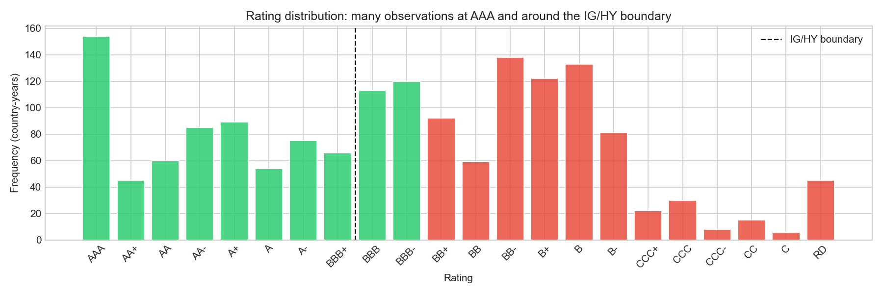

To support the visual interpretation, we summarise a few economically meaningful parts of the rating scale.

total_obs = len(sovereign)

aaa_obs = rating_counts['AAA']

a_bands = ['A+','A','A-','BBB+','BBB','BBB-']
bb_bands = ['BB+','BB','BB-','B+','B','B-']
boundary_bands = ['BBB+','BBB','BBB-','BB+','BB','BB-']
distress_bands = ['CCC+','CCC','CCC-','CC','C','RD']

summary_stats = pd.DataFrame({
    'Group': [
        'AAA only',
        'A/BBB bands',
        'BB/B bands',
        'Near IG/HY boundary (BBB & BB bands)',
        'CCC and below'
    ],
    'Observations': [
        aaa_obs,
        rating_counts[a_bands].sum(),
        rating_counts[bb_bands].sum(),
        rating_counts[boundary_bands].sum(),
        rating_counts[distress_bands].sum()
    ]
})

summary_stats['Share of sample (%)'] = 100 * summary_stats['Observations'] / total_obs
summary_stats['Share of sample (%)'] = summary_stats['Share of sample (%)'].round(1)

print(summary_stats.to_string(index=False))

boundary_detail = rating_counts[['BBB+','BBB','BBB-','BB+','BB','BB-']].reset_index()
boundary_detail.columns = ['Rating', 'Count']
print("\nBoundary bands:")
print(boundary_detail.to_string(index=False))

print(f"\nTotal observations: {total_obs}")
print(f"Investment-grade share: {(sovereign['is_ig'].mean() * 100):.1f}%")
print(f"Non-investment-grade share: {((1 - sovereign['is_ig'].mean()) * 100):.1f}%")

                           Group  Observations  Share of sample (%)
                        AAA only           154                  9.6
                     A/BBB bands           517                 32.1
                      BB/B bands           625                 38.8
Near IG/HY boundary (BBB & BB bands)           588                 36.5
                   CCC and below           126                  7.8

Boundary bands:
Rating  Count
  BBB+     66
   BBB    113
  BBB-    120
   BB+     92
    BB     59
   BB-    138

Total observations: 1612
Investment-grade share: 53.4%
Non-investment-grade share: 46.6%

Because the AAA spike is visually striking, it is useful to check whether it reflects many countries appearing briefly at the top of the scale, or a smaller set of countries remaining there for many years.

aaa_df = sovereign[sovereign['rating'] == 'AAA'].copy()

aaa_country_summary = (
    aaa_df.groupby('country_clean')
    .agg(
        aaa_years=('year', 'count'),
        first_aaa_year=('year', 'min'),
        last_aaa_year=('year', 'max')
    )
    .sort_values('aaa_years', ascending=False)
)

print(f"Countries ever rated AAA: {aaa_country_summary.shape[0]}")
print(f"AAA observations: {len(aaa_df)}")
print(f"Mean AAA years per AAA-rated country: {aaa_country_summary['aaa_years'].mean():.2f}")
print(f"Median AAA years per AAA-rated country: {aaa_country_summary['aaa_years'].median():.1f}")

print("\nTop AAA countries by number of AAA years:")
print(aaa_country_summary.head(10).to_string())

Countries ever rated AAA: 15
AAA observations: 154
Mean AAA years per AAA-rated country: 10.27
Median AAA years per AAA-rated country: 14.0

Top AAA countries by number of AAA years:
                          aaa_years  first_aaa_year  last_aaa_year
country_clean                                                     
Australia                        14            2012           2025
Denmark                          14            2012           2025
Germany                          14            2012           2025
Luxembourg                       14            2012           2025
Netherlands                      14            2012           2025
Norway                           14            2012           2025
Singapore                        14            2012           2025
Sweden                           14            2012           2025
Switzerland                      14            2012           2025
United States of America         11            2012           2022

The rating distribution spans almost the entire Fitch scale, from AAA down to RD, so the dataset covers a wide range of sovereign credit quality rather than a narrow subset of countries. At the same time, the observations are not evenly distributed across the scale. Two features stand out clearly: a sizeable AAA block and a broad concentration in the middle of the scale, especially around the investment-grade / high-yield boundary.

The AAA category alone accounts for 154 country-year observations, or 9.6% of the full sample. A country-level check shows that these observations are concentrated among only 15 countries. The median AAA-rated country is observed at AAA for the full 14-year sample window, while the mean is lower at 10.3 years because a smaller number of countries spend fewer years at AAA, pulling the average down. In other words, the AAA spike is driven mainly by a core group of sovereigns that remain at the top of the scale for most or all of the sample period. Several sovereigns, including Australia, Denmark, Germany, Luxembourg, the Netherlands, Norway, Singapore, Sweden, and Switzerland, remain at AAA throughout the full 2012–2025 window. For the binary task of predicting investment-grade versus non-investment-grade status, these are likely to be among the least ambiguous cases. Economically, that is what we would expect: sovereigns at the top of the rating scale are associated with exceptionally strong repayment capacity, deep institutional credibility, and very low perceived default risk.

The middle of the scale is even more important for the modelling problem. The A/BBB bands account for 32.1% of the sample, while the BB/B bands account for 38.8%. This means the dataset is not dominated only by obvious extremes. Instead, a large share of observations lies in the part of the rating spectrum where the distinction between the two classes is more economically meaningful and potentially more difficult.

Most importantly, 36.5% of all country-year observations lie directly in the BBB and BB bands, i.e. in the six notches closest to the IG/HY boundary. The boundary detail confirms that this region is heavily populated, with especially large counts in BBB- (120 observations) and BB- (138 observations), as well as substantial mass in BBB (113) and BB+ (92). These are precisely the observations most relevant for a binary IG/non-IG classification task: sovereigns in BBB are on the investment-grade side but close to the cutoff, while sovereigns in BB are just below it. They are therefore the cases where moderate changes in debt sustainability, fiscal credibility, external vulnerability, or political risk may be enough to change whether a sovereign is considered investment-grade.

On the speculative-grade side more broadly, the BB/B block is larger than the A/BBB block (38.8% versus 32.1%), which shows that the non-investment-grade class is not made up only of rare distress cases. It contains a substantial number of countries in the upper speculative grades, which are exactly the comparison cases that matter when trying to distinguish borderline investment-grade sovereigns from borderline non-investment-grade ones. Economically, this is the region of the rating scale where investor confidence, refinancing conditions, and macro-policy credibility are often most sensitive to deterioration in fundamentals.

By contrast, the severe-distress tail is relatively small: CCC and below account for only 7.8% of observations. These cases are economically important, but from a binary IG/non-IG perspective they are usually less ambiguous than the borderline BBB/BB cases.

Finally, the binary class split itself is fairly balanced: 53.4% of observations are investment-grade and 46.6% are non-investment-grade. This is useful for modelling, because it means the task is not driven by overwhelming class imbalance. The main difficulty comes instead from the large number of observations clustered around the threshold.

Modelling implication: the dataset contains both easy cases (such as the persistent AAA sovereigns) and a very large number of economically important borderline cases near the IG/HY boundary. Since more than a third of the sample lies in the BBB/BB region, model performance should be judged not only by overall accuracy, but also by how well the model handles the cases closest to the classification threshold.

Q2.3.2: Rating switches over time

We now examine how often sovereign ratings actually change from one year to the next.

sovereign['prev_rating'] = sovereign.groupby('country_clean')['rating'].shift(1)
sovereign['rating_changed'] = (
    (sovereign['rating'] != sovereign['prev_rating']) &
    sovereign['prev_rating'].notna()
)

changes = sovereign[sovereign['rating_changed']]

print(f"Total rating changes: {len(changes)}")
print(f"Mean per year: {changes.groupby('year')['rating_changed'].sum().mean():.1f}")
print(f"As % of all obs: {len(changes)/len(sovereign)*100:.1f}%")
print(f"\nChanges per year:")
print(changes.groupby('year')['rating_changed'].sum().to_string())

Total rating changes: 300
Mean per year: 23.1
As % of all obs: 18.6%

Changes per year:
2013    28
2014    22
2015    19
2016    31
2017    25
2018    21
2019    25
2020    33
2021    14
2022    27
2023    25
2024    27
2025     3

There are 300 rating changes in total, corresponding to an average of about 23 changes per year. Put differently, only 18.6% of country-year observations involve any change in the raw Fitch rating at all. So sovereign ratings are not completely static, but they are still highly persistent relative to the size of the panel: in more than four-fifths of observations, the prevailing rating is unchanged from the previous year.

This matters economically because sovereign ratings are designed to be through-the-cycle assessments rather than highly reactive market prices. Agencies do revise them when fiscal conditions, external balances, governance, default risk, or political events materially alter creditworthiness, but they do not usually move them every year. That persistence means the current rating already contains substantial information about the likely rating next year.

The timing of rating changes is also not uniform across years. The largest number of changes occurs in 2020 (33 changes), which is consistent with the broad sovereign stress created by the COVID shock. The relatively high counts in 2016, 2022, 2023, and 2024 also suggest periods of heightened reassessment. By contrast, the very low count in 2025 almost certainly reflects incomplete coverage at the end of the sample rather than a genuine collapse in rating activity.

To go beyond simple frequency counts, we next examine the size of rating changes measured in notches. To make the sign convention intuitive, we define the notch change so that positive values indicate upgrades and negative values indicate downgrades.

rating_codes = {r: i for i, r in enumerate(rating_order)}
sovereign['rating_code'] = sovereign['rating'].map(rating_codes)
sovereign['prev_code']   = sovereign.groupby('country_clean')['rating_code'].shift(1)

# Positive = upgrade (better rating), negative = downgrade (worse rating)
sovereign['notch_change'] = sovereign['prev_code'] - sovereign['rating_code']

changes_only = sovereign.loc[sovereign['rating_changed'], 'notch_change'].dropna()

one_notch_share = (changes_only.abs() == 1).mean() * 100
two_notch_share = (changes_only.abs() == 2).mean() * 100
large_move_share = (changes_only.abs() >= 3).mean() * 100

print(f"Single-notch changes: {one_notch_share:.1f}%")
print(f"Two-notch changes: {two_notch_share:.1f}%")
print(f"Three-or-more-notch changes: {large_move_share:.1f}%")
print(f"Min notch change: {changes_only.min():.0f}")
print(f"Max notch change: {changes_only.max():.0f}")

Single-notch changes: 76.7%
Two-notch changes: 14.0%
Three-or-more-notch changes: 9.3%
Min notch change: -12
Max notch change: 7

fig, ax = plt.subplots(figsize=(9, 4))
ax.hist(
    changes_only,
    bins=range(int(changes_only.min()) - 1, int(changes_only.max()) + 2),
    color='steelblue',
    edgecolor='white',
    alpha=0.85
)
ax.axvline(0, color='red', linestyle='--', linewidth=0.8)
ax.set_title('One-notch moves dominate: large jumps are rare (76.7% of changes are single-notch)')
ax.set_xlabel('Notch change (positive = upgrade, negative = downgrade)')
ax.set_ylabel('Count')
plt.tight_layout()
plt.show()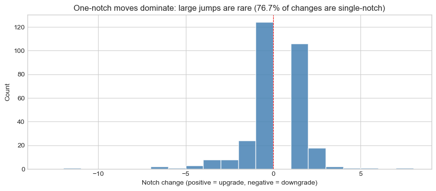

The distribution is heavily concentrated around ±1 notch: 76.7% of all observed changes are single-notch moves, 14.0% are two-notch moves, and only 9.3% involve changes of three notches or more. This is consistent with how rating agencies generally operate. Rating revisions are usually incremental, with agencies moving cautiously as credit fundamentals evolve rather than making large jumps in normal times.

Large multi-notch moves do occur, but they are rare and typically associated with acute crises, default episodes, or major geopolitical shocks. In this annual panel, the most extreme case is Russia in 2022, which moves from BBB to C, a 12-notch downgrade following the invasion of Ukraine and the imposition of sanctions. Other large deteriorations include cases such as Belarus (−7 notches), Ghana (−6), Ukraine (−5), Suriname (−5), and Venezuela (−4), all linked to severe financial or political stress. Large upward moves also appear in a few exceptional cases: for example, Argentina records a +7-notch upgrade from RD to B in 2016.

That last example highlights an important interpretation point. Because the dataset records the prevailing rating in each country-year, the notch change measures the net year-to-year movement, not necessarily a single discrete rating action. A country may experience several actions within one year, but the annual panel only captures the difference between the prevailing rating in year $t-1$ and year $t$. This helps explain why some episodes may appear smaller or larger than expected from the underlying event chronology. For example, Argentina’s deterioration is spread across several annual moves in the panel, rather than appearing as one single collapse in a single year.

To make the persistence of the binary target explicit, we now check how many of these raw rating changes actually produce a change in investment-grade status.

Q2.3.3: Do all rating changes result in IG status changes?

We compute the investment-grade transition matrix directly.

sovereign['prev_ig'] = sovereign.groupby('country_clean')['is_ig'].shift(1)
ig_trans = sovereign.dropna(subset=['prev_ig'])

transition_matrix = ig_trans.groupby(['prev_ig','is_ig']).size().unstack(fill_value=0)
print(transition_matrix)

is_ig      0    1
prev_ig          
0.0      678    8
1.0       14  787

We can also express these counts as shares of the modelling panel.

transition_counts = pd.DataFrame({
    'Transition': [
        'Stayed non-IG',
        'non-IG → IG (upgrade)',
        'IG → non-IG (downgrade)',
        'Stayed IG'
    ],
    'Count': [678, 8, 14, 787]
})
transition_counts['Share (%)'] = 100 * transition_counts['Count'] / transition_counts['Count'].sum()
transition_counts['Share (%)'] = transition_counts['Share (%)'].round(1)

print(transition_counts.to_string(index=False))

crossings = transition_counts.loc[
    transition_counts['Transition'].isin(['non-IG → IG (upgrade)', 'IG → non-IG (downgrade)']),
    'Count'
].sum()

print(f"\nTotal IG threshold crossings: {crossings}")
print(f"Share of all country-years: {100 * crossings / transition_counts['Count'].sum():.1f}%")
print(f"Persistence benchmark ('same as current year'): {100 * (1 - crossings / transition_counts['Count'].sum()):.1f}%")

             Transition  Count  Share (%)
        Stayed non-IG    678       45.6
non-IG → IG (upgrade)      8        0.5
IG → non-IG (downgrade)   14        0.9
           Stayed IG     787       52.9

Total IG threshold crossings: 22
Share of all country-years: 1.5%
Persistence benchmark ('same as current year'): 98.5%

Only 22 observations (1.5%) involve a crossing of the investment-grade threshold. The remaining 1,465 observations (98.5%) stay on the same side of the IG/non-IG boundary as the previous year.

This immediately shows that the binary target is even more persistent than the raw letter ratings. We can make that comparison explicit by checking how many of the 300 raw rating changes stay within the same binary class.

# Compute previous-year IG status on the full panel first
sovereign['prev_ig'] = sovereign.groupby('country_clean')['is_ig'].shift(1)

# Then restrict to rows where the raw rating changed
changes = sovereign[sovereign['rating_changed']].copy()

within_tier_changes = (changes['prev_ig'] == changes['is_ig']).sum()
cross_tier_changes = (changes['prev_ig'] != changes['is_ig']).sum()

print(f"Total raw rating changes: {len(changes)}")
print(f"Within-tier changes: {within_tier_changes} ({100 * within_tier_changes / len(changes):.1f}%)")
print(f"Cross-tier changes: {cross_tier_changes} ({100 * cross_tier_changes / len(changes):.1f}%)")

Total raw rating changes: 300
Within-tier changes: 278 (92.7%)
Cross-tier changes: 22 (7.3%)

This is the key link between the two subsections. Although there are 300 raw rating changes in the panel, 278 of them (92.7%) are within-tier moves that do not alter investment-grade status. These include changes such as BBB → BBB+ (stays IG) or BB → B+ (stays non-IG). So the majority of rating actions are economically meaningful as changes in credit quality, but not as changes in the binary classification target.

This finding is central for the modelling task. A very simple persistence rule, i.e predict that next year’s IG status will be the same as this year’s, would already be correct 98.5% of the time. Any evaluation metric that ignores this will therefore be misleading. A model can achieve very high raw accuracy simply by exploiting persistence, without learning much about the rare but economically important threshold-crossing cases.

For completeness, the actual IG threshold crossings in the panel are:

# Identify actual IG threshold crossings
crossings_df = sovereign.copy()
crossings_df['prev_rating'] = crossings_df.groupby('country_clean')['rating'].shift(1)
crossings_df['prev_ig'] = crossings_df.groupby('country_clean')['is_ig'].shift(1)

ig_crossings = crossings_df[
    crossings_df['prev_ig'].notna() &
    (crossings_df['prev_ig'] != crossings_df['is_ig'])
][['country_clean', 'year', 'prev_rating', 'rating', 'prev_ig', 'is_ig']].copy()

ig_crossings['Direction'] = np.where(
    (ig_crossings['prev_ig'] == 0) & (ig_crossings['is_ig'] == 1),
    'non-IG → IG',
    'IG → non-IG'
)

ig_crossings = ig_crossings.rename(columns={
    'country_clean': 'Country',
    'year': 'Year',
    'prev_rating': 'Old Rating',
    'rating': 'New Rating'
})

ig_crossings = ig_crossings.sort_values(['Year', 'Country']).reset_index(drop=True)

print(ig_crossings[['Country', 'Year', 'Old Rating', 'New Rating', 'Direction']].to_markdown(index=False))

Country	Year	Old Rating	New Rating	Direction
Croatia	2013	BBB-	BB+	IG → non-IG
Philippines	2013	BB+	BBB-	non-IG → IG
Uruguay	2013	BB+	BBB-	non-IG → IG
Brazil	2015	BBB	BB+	IG → non-IG
Azerbaijan	2016	BBB-	BB+	IG → non-IG
Bahrain	2016	BBB-	BB+	IG → non-IG
Hungary	2016	BB+	BBB-	non-IG → IG
Namibia	2017	BBB-	BB+	IG → non-IG
Portugal	2017	BB+	BBB	non-IG → IG
South Africa	2017	BBB-	BB+	IG → non-IG
Türkiye	2017	BBB-	BB+	IG → non-IG
Cyprus	2018	BB	BBB-	non-IG → IG
Oman	2018	BBB-	BB+	IG → non-IG
Croatia	2019	BB+	BBB-	non-IG → IG
Aruba	2020	BBB-	BB	IG → non-IG
Morocco	2020	BBB-	BB+	IG → non-IG
San Marino	2020	BBB-	BB+	IG → non-IG
Colombia	2021	BBB-	BB+	IG → non-IG
Russian Federation	2022	BBB	C	IG → non-IG
Greece	2023	BB	BBB-	non-IG → IG
Azerbaijan	2024	BB+	BBB-	non-IG → IG
Panama	2024	BBB-	BB+	IG → non-IG

These threshold crossings line up with major macroeconomic and political turning points. Brazil 2015 reflects fiscal deterioration and domestic political crisis. Colombia 2021 reflects post-pandemic fiscal stress. Greece 2023 marks recovery after a long post-crisis period below investment grade. Russia 2022 is the most extreme case: a multi-notch downgrade driven by a discrete geopolitical shock and sanctions following the invasion of Ukraine, rather than by gradual deterioration in the prior year’s macro indicators. This is a useful reminder of the fundamental limit of macro-based forecasting: some rating events are driven by sudden political or geopolitical breaks that are very difficult to anticipate from lagged economic fundamentals alone.

Modelling implication: the raw rating scale shows some movement over time, but the binary IG/non-IG target is extraordinarily persistent. The central modelling challenge is therefore not predicting whether ratings change at all. It is predicting the very small set of cases in which countries cross the BBB− / BB+ threshold. That is why overall accuracy alone is a poor evaluation metric, and why the persistence benchmark must be made explicit before any classifier is estimated.

Q2.3.4: Cross-sectional comparison of IG and Non-IG sovereigns

To understand which country characteristics are most strongly associated with investment-grade status, we compare the median values of several macroeconomic and institutional indicators across the two groups.

macro_vars = ['NY.GDP.MKTP.KD.ZG','BN.CAB.XOKA.GD.ZS','GGXWDG_NGDP',
              'GE.EST','CC.EST','RL.EST']

# Use medians for robustness against extreme outliers
comparison = model_df.groupby('is_ig')[macro_vars].median()
print(comparison.T.rename(columns={0:'Non-IG', 1:'IG'}).round(2).to_string())

# Inflation: compute YoY % change within each country
# PCPI levels are not cross-country comparable because they are in local units
model_df_sorted = model_df.sort_values(['country_clean','year']).copy()
model_df_sorted['inflation_pct'] = (
    model_df_sorted.groupby('country_clean')['PCPI'].pct_change() * 100
)

print("\nMedian inflation rate (YoY %) by IG:")
print(model_df_sorted.groupby('is_ig')['inflation_pct'].median().rename({0:'Non-IG', 1:'IG'}).round(2))

is_ig              Non-IG     IG
NY.GDP.MKTP.KD.ZG    3.42   2.64
BN.CAB.XOKA.GD.ZS   -2.94   0.94
GGXWDG_NGDP         58.99  49.65
GE.EST              -0.33   1.02
CC.EST              -0.48   0.78
RL.EST              -0.37   0.96

Median inflation rate (YoY %) by IG:
is_ig
Non-IG    4.45
IG        2.14
Name: inflation_pct, dtype: float64

Note

Note on inflation measurement: The IMF WEO PCPI variable is the average Consumer Price Index. Its level is expressed in country-specific units and is therefore not directly comparable across countries. We therefore convert it into a within-country year-on-year inflation rate using the percentage change in PCPI, and compare medians rather than means so that hyperinflation episodes do not dominate the summary.

Because these variables are measured in different units, raw median gaps are not directly comparable across indicators. To compare the strength of separation more meaningfully, we therefore scale each median gap by the variable’s interquartile range (IQR). This produces a unit-free measure of how far apart the IG and non-IG medians are relative to the typical spread of the variable.

indicator_map = {
    'NY.GDP.MKTP.KD.ZG': 'GDP growth (%)',
    'BN.CAB.XOKA.GD.ZS': 'Current account (% GDP)',
    'GGXWDG_NGDP': 'Government debt (% GDP)',
    'GE.EST': 'Government effectiveness',
    'CC.EST': 'Control of corruption',
    'RL.EST': 'Rule of law'
}

plot_df = model_df_sorted.copy()

vars_for_gap = [
    'NY.GDP.MKTP.KD.ZG',
    'BN.CAB.XOKA.GD.ZS',
    'GGXWDG_NGDP',
    'GE.EST',
    'CC.EST',
    'RL.EST',
    'inflation_pct'
]

label_map = {
    **indicator_map,
    'inflation_pct': 'Inflation (YoY %)'
}

rows = []
for var in vars_for_gap:
    med_ig = plot_df.loc[plot_df['is_ig'] == 1, var].median()
    med_non = plot_df.loc[plot_df['is_ig'] == 0, var].median()
    q75 = plot_df[var].quantile(0.75)
    q25 = plot_df[var].quantile(0.25)
    iqr = q75 - q25

    rows.append({
        'Indicator': label_map[var],
        'IG median': med_ig,
        'Non-IG median': med_non,
        'Raw gap (IG - Non-IG)': med_ig - med_non,
        'IQR': iqr,
        'IQR-normalised gap': (med_ig - med_non) / iqr if iqr != 0 else np.nan
    })

gap_norm_df = pd.DataFrame(rows).sort_values('IQR-normalised gap')

print(
    gap_norm_df[
        ['Indicator', 'Raw gap (IG - Non-IG)', 'IQR', 'IQR-normalised gap']
    ].round(3).to_string(index=False)
)

fig, ax = plt.subplots(figsize=(8, 5))
ax.barh(gap_norm_df['Indicator'], gap_norm_df['IQR-normalised gap'], alpha=0.85)
ax.axvline(0, color='black', linewidth=0.8)
ax.set_title('Median difference (IG minus non-IG), normalised by IQR')
ax.set_xlabel('Median gap / IQR')
plt.tight_layout()
plt.show()

Indicator  Raw gap (IG - Non-IG)    IQR  IQR-normalised gap
       Inflation (YoY %)                 -2.315  4.687              -0.494
 Government debt (% GDP)                 -9.335 40.465              -0.231
          GDP growth (%)                 -0.780  3.890              -0.201
 Current account (% GDP)                  3.879  6.542               0.593
   Control of corruption                  1.258  1.561               0.806
             Rule of law                  1.337  1.505               0.888
Government effectiveness                  1.347  1.407               0.958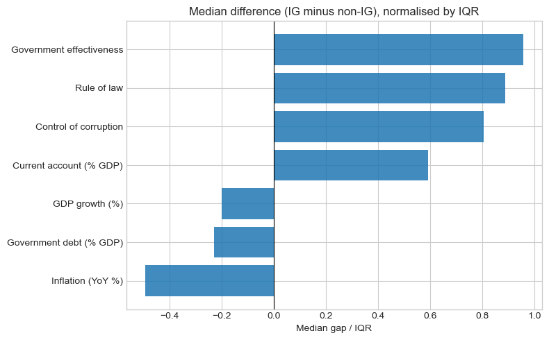

The raw medians already show clear contrasts between the two groups.

Indicator	IG (median)	Non-IG (median)	Interpretation
GDP Growth (%)	2.64	3.42	Non-IG countries have slightly higher median growth. This should not be interpreted as stronger credit fundamentals. Faster growth among non-IG sovereigns often reflects catch-up growth from lower income levels, whereas ratings depend more on macro stability and repayment capacity than on raw growth alone.
Current Account (% GDP)	+0.94	−2.94	This is one of the clearest macroeconomic differences. IG sovereigns run a small median surplus, while non-IG sovereigns run a median deficit of almost 3% of GDP. Persistent external deficits can increase dependence on foreign financing and make countries more vulnerable to sudden stops or refinancing stress.
Government Debt (% GDP)	49.65	58.99	Non-IG sovereigns have higher median public debt, but the gap is moderate rather than overwhelming. This suggests debt matters, but not on its own: what matters for ratings is not only the stock of debt, but whether markets believe the country can manage and service it credibly.
Inflation rate (YoY %)	2.14	4.45	Median inflation is more than twice as high in non-IG sovereigns. This points to weaker nominal stability and lower policy credibility, both of which matter for sovereign risk because they can feed into exchange-rate stress, financing pressure, and debt-servicing difficulties.
Government Effectiveness	+1.02	−0.33	This is one of the largest raw gaps in the table. On the WGI scale (roughly −2.5 to +2.5), a difference of about 1.35 points is substantial. IG sovereigns are associated with much stronger policy implementation capacity and state effectiveness.
Control of Corruption	+0.78	−0.48	The corruption gap is also large, at about 1.26 points. Better corruption control is associated with stronger fiscal capacity, better public administration, and greater investor confidence.
Rule of Law	+0.96	−0.37	The rule-of-law gap is similarly wide, at about 1.33 points. Stronger legal institutions support contract enforcement, policy predictability, and broader macro-financial stability.

The IQR-normalised gap plot sharpens the interpretation. Once the median differences are scaled by the typical dispersion of each variable, the governance indicators, especially Government Effectiveness, Rule of Law, and Control of Corruption, emerge as some of the strongest sources of separation between IG and non-IG sovereigns. The current account also shows substantial separation, while inflation and government debt remain clearly worse in the non-IG group. By contrast, GDP growth shows relatively little useful separation once scaled in the same way, and the sign is actually reversed, with non-IG sovereigns growing slightly faster on average.

This makes the economic picture clearer. Investment-grade status is not simply a story of faster growth or mechanically lower debt. Instead, IG sovereigns differ from non-IG sovereigns along three broader dimensions:

stronger institutions, as shown by the large governance gaps
greater external stability, reflected in the current-account difference
more credible nominal frameworks, reflected in lower inflation

That interpretation is economically plausible. Rating agencies assess not only a country’s ability to repay, which depends on growth, fiscal space, inflation control, and external balances, but also its credibility and resilience, which are closely tied to governance. A sovereign with moderate debt but weak institutions may still be rated non-investment-grade if markets doubt the consistency or reliability of policy. Conversely, stronger institutions can help sustain investment-grade status even when debt is not especially low.

The growth result is also instructive. Non-IG sovereigns have slightly higher median GDP growth (3.42% versus 2.64%), but this does not mean they are safer credits. Ratings are much more closely related to stability, repayment capacity, and institutional credibility than to raw growth rates alone. A fast-growing but institutionally weak sovereign can still be risky, especially if growth is volatile or financed by persistent external deficits.

The current-account and inflation figures reinforce this point. Relative to IG sovereigns, non-IG countries have weaker external positions and less price stability. These patterns are exactly what one would expect if weaker-rated sovereigns face more fragile macroeconomic environments and lower policy credibility.

Key insight: once the gaps are made comparable across variables, the strongest descriptive differences between IG and non-IG sovereigns are concentrated in institutional quality, with important supporting roles for external balance and inflation stability. This suggests that a predictive model for IG status should not focus only on macroeconomic performance in the narrow sense, but also on the governance environment in which fiscal and external adjustment takes place.

Q2.3.5: Multi-variable visualisation

To move beyond one-variable-at-a-time summaries, we now compare one institutional indicator and one fiscal indicator jointly. The aim is to see whether investment-grade and non-investment-grade sovereigns separate clearly in a simple two-dimensional space, or whether substantial overlap remains.

# Prepare data
plot_df = model_df[['is_ig', 'GE.EST', 'GGXWDG_NGDP', 'country_clean', 'year', 'rating']].dropna().copy()
plot_df['IG status'] = plot_df['is_ig'].map({1: 'IG', 0: 'Non-IG'})

# 💜 Accessible purple-based palette
accessible_colors = {
    'Non-IG': '#8e44ad',      # Deep purple
    'IG': '#00a087'   # Teal complement
}

fig = px.scatter(
    plot_df,
    x='GE.EST',
    y='GGXWDG_NGDP',
    color='IG status',
    color_discrete_map=accessible_colors,
    hover_data={
        'country_clean': True,
        'year': True,
        'rating': True,
        'GE.EST': ':.2f',
        'GGXWDG_NGDP': ':.2f',
        'IG status': False
    },
    labels={
        'GE.EST': 'Government Effectiveness (WB Governance Indicator, −2.5 to +2.5)',
        'GGXWDG_NGDP': 'Gross Government Debt (% of GDP)',
        'IG status': 'Investment Grade Status'
    },
    title='IG and non-IG separate more clearly by institutional quality than by debt burden alone'
)

# 🎯 STEP 1: Add the horizontal reference line
fig.add_hline(
    y=60,
    line_dash='dash',
    line_color='#5d4a66',
    line_width=2,
    opacity=0.8
)

# 🎯 STEP 2: Add SIMPLE text annotation NEXT TO the line
fig.add_annotation(
    x=0.015, y=60,
    xref='paper', yref='y',
    text='60% debt line',
    showarrow=False,
    font=dict(size=12, family='Arial, sans-serif', color='#5d4a66'),
    bgcolor='rgba(255, 255, 255, 0.9)',
    borderpad=3,
    align='left',
    opacity=0.95
)

# ✨ Marker styling
fig.update_traces(
    marker=dict(
        size=11,
        opacity=0.75,
        line=dict(width=1.2, color='white')
    ),
    selector=dict(mode='markers')
)

# 🎨 Layout
fig.update_layout(
    width=1000,
    height=650,
    
    # Legend: colored markers, inside plot
    legend=dict(
        title='',
        orientation='v',
        x=0.98, y=0.98,
        xanchor='right', yanchor='top',
        bgcolor='rgba(255, 255, 255, 0.85)',
        bordercolor='#5d4a66',
        borderwidth=1,
        font=dict(size=10, family='Arial, sans-serif'),
        itemsizing='constant'
    ),
    
    template='plotly_white',
    
    hoverlabel=dict(
        bgcolor='white',
        bordercolor='#8e44ad',
        font=dict(size=11, family='Arial, sans-serif')
    ),
    
    xaxis=dict(
        gridcolor='rgba(142, 68, 173, 0.12)',
        zerolinecolor='rgba(0,0,0,0.15)',
        title_font=dict(size=12, family='Arial, sans-serif'),
        tickfont=dict(size=10),
        showline=True,
        linewidth=1,
        linecolor='rgba(0,0,0,0.2)'
    ),
    
    yaxis=dict(
        gridcolor='rgba(142, 68, 173, 0.12)',
        zerolinecolor='rgba(0,0,0,0.15)',
        title_font=dict(size=12, family='Arial, sans-serif'),
        tickfont=dict(size=10),
        showline=True,
        linewidth=1,
        linecolor='rgba(0,0,0,0.2)',
        range=[0, max(plot_df['GGXWDG_NGDP']) * 1.12]
    ),
    
    # ✅ Title styling to accommodate longer, informative text
    title=dict(
        text='IG and non-IG separate more clearly by institutional quality than by debt burden alone',
        font=dict(size=13, family='Arial, sans-serif', color='#2c3e50'),
        x=0.5,
        xanchor='center',
        pad=dict(t=10, b=5)
    ),
    
    plot_bgcolor='rgba(250, 248, 252, 0.5)',
    paper_bgcolor='white'
)

fig.show()
fig.write_html('ig-scatter-purple-interactive.html')

To inspect the middle of the figure more carefully, we also extract observations with government effectiveness between −0.5 and +0.5 and debt between 40% and 80% of GDP.

boundary_cases = plot_df[
    plot_df['GE.EST'].between(-0.5, 0.5) &
    plot_df['GGXWDG_NGDP'].between(40, 80)
].sort_values(['is_ig', 'GE.EST', 'GGXWDG_NGDP'])

print(boundary_cases[['country_clean', 'year', 'rating', 'is_ig', 'GE.EST', 'GGXWDG_NGDP']]
      .rename(columns={'is_ig': 'IG status'})
      .to_string(index=False))

country_clean  year rating  IG status    GE.EST  GGXWDG_NGDP
           Ukraine  2022     CC          0 -0.497119       77.717
           Ecuador  2023   CCC+          0 -0.494245       54.332
             Kenya  2018     B+          0 -0.493653       56.449
             Benin  2019      B          0 -0.490368       40.375
       El Salvador  2018     B-          0 -0.489994       76.961
Dominican Republic  2013      B          0 -0.488939       46.809
          Maldives  2018     B+          0 -0.475938       70.653
          Mongolia  2023      B          0 -0.471536       46.705
           Ecuador  2020     B-          0 -0.470506       63.551
          Paraguay  2023    BB+          0 -0.462065       41.060
           Ukraine  2018     B-          0 -0.459632       60.353
           Lesotho  2013    BB-          0 -0.457246       41.192
Dominican Republic  2014     B+          0 -0.456835       45.022
          Tanzania  2023     B+          0 -0.455081       47.804
          Mongolia  2015      B          0 -0.448192       50.547
          Ethiopia  2014      B          0 -0.443245       44.152
             Kenya  2019     B+          0 -0.441659       59.085
           Ukraine  2021      B          0 -0.439536       48.917
          Pakistan  2021     B-          0 -0.438822       74.749
          Mongolia  2014     B+          0 -0.426088       43.963
          Mongolia  2022      B          0 -0.424925       64.568
           Ukraine  2020      B          0 -0.410091       60.505
             Kenya  2016     B+          0 -0.402431       50.399
             Kenya  2020     B+          0 -0.399473       67.959
           Ukraine  2014    CCC          0 -0.398847       70.317
           Bolivia  2017    BB-          0 -0.395565       51.260
Dominican Republic  2015     B+          0 -0.394820       44.812
          Maldives  2017     B+          0 -0.394718       63.752
             Kenya  2015     B+          0 -0.393977       45.832
             Kenya  2017     B+          0 -0.390357       53.866
Dominican Republic  2018    BB-          0 -0.388736       50.798
       El Salvador  2017     B-          0 -0.387302       77.136
           Ecuador  2016      B          0 -0.383571       46.066
Dominican Republic  2017    BB-          0 -0.383381       49.480
          Suriname  2015    BB-          0 -0.379115       41.175
          Suriname  2016     B+          0 -0.372117       75.395
           Ecuador  2019     B-          0 -0.367696       52.064
             Kenya  2014     B+          0 -0.358902       41.281
           Belarus  2017     B-          0 -0.357744       53.160
           Ecuador  2017      B          0 -0.352248       47.391
Dominican Republic  2019    BB-          0 -0.351295       53.456
       El Salvador  2016     B+          0 -0.343923       75.214
           Ukraine  2019      B          0 -0.334267       50.452
           Armenia  2015     B+          0 -0.331790       48.276
           Bolivia  2018    BB-          0 -0.329585       53.076
             Kenya  2022      B          0 -0.329533       67.800
             Kenya  2021     B+          0 -0.325909       68.232
             Ghana  2018      B          0 -0.319947       61.976
             Ghana  2015      B          0 -0.319786       53.896
           Ecuador  2018     B-          0 -0.317794       49.505
           Armenia  2022     B+          0 -0.314792       49.279
           Armenia  2016     B+          0 -0.312554       56.476
           Ecuador  2022     B-          0 -0.309278       57.203
             Ghana  2014      B          0 -0.307953       50.111
           Armenia  2020     B+          0 -0.304547       67.271
             Kenya  2023      B          0 -0.303605       73.405
           Belarus  2018      B          0 -0.297943       47.515
             Benin  2020      B          0 -0.290914       46.142
Dominican Republic  2016    BB-          0 -0.290740       46.685
             Ghana  2019      B          0 -0.289961       62.927
       El Salvador  2015     B+          0 -0.285931       73.464
           Armenia  2021     B+          0 -0.282197       63.649
Dominican Republic  2020    BB-          0 -0.281448       71.812
           Armenia  2014    BB-          0 -0.257330       43.631
      South Africa  2023    BB-          0 -0.256947       73.220
            Brazil  2015    BB+          0 -0.255272       71.730
         Argentina  2013     CC          0 -0.254237       43.496
             Ghana  2016      B          0 -0.254053       55.942
           Armenia  2017     B+          0 -0.251550       58.093
            Brazil  2016     BB          0 -0.249387       77.422
          Mongolia  2018      B          0 -0.246418       76.539
           Vietnam  2013     B+          0 -0.245402       41.413
           Ecuador  2021     B-          0 -0.241594       61.756
             Benin  2021     B+          0 -0.237601       50.288
          Mongolia  2019      B          0 -0.234439       66.837
           Armenia  2019    BB-          0 -0.226046       54.152
             Benin  2023     B+          0 -0.218984       54.904
           Tunisia  2021     B-          0 -0.207107       79.728
         Argentina  2012     CC          0 -0.206967       40.436
           Tunisia  2016    BB-          0 -0.206499       58.908
         Sri Lanka  2012    BB-          0 -0.204319       67.504
             Ghana  2020      B          0 -0.196979       79.089
             Ghana  2017      B          0 -0.187149       56.984
           Tunisia  2020      B          0 -0.186425       77.708
           Morocco  2020    BB+          0 -0.186066       72.245
           Armenia  2023    BB-          0 -0.184130       50.449
            Serbia  2013    BB-          0 -0.179091       54.102
          Maldives  2019     B+          0 -0.175837       77.203
           Belarus  2019      B          0 -0.174483       40.999
         Sri Lanka  2017     B+          0 -0.174113       72.260
            Serbia  2012    BB-          0 -0.173352       51.727
             Benin  2022     B+          0 -0.170590       54.187
           Armenia  2018     B+          0 -0.170583       56.069
           Morocco  2021    BB+          0 -0.170099       69.351
         Sri Lanka  2013    BB-          0 -0.166648       69.457
              Oman  2021    BB-          0 -0.155151       61.873
       El Salvador  2012     BB          0 -0.134836       69.994
             Ghana  2013      B          0 -0.134415       42.930
   North Macedonia  2019    BB+          0 -0.124041       40.448
   North Macedonia  2021    BB+          0 -0.121814       52.750
       El Salvador  2013    BB-          0 -0.121621       69.655
         Argentina  2014     RD          0 -0.111114       44.697
      South Africa  2022    BB-          0 -0.109028       70.715
           Tunisia  2015    BB-          0 -0.102188       52.401
          Mongolia  2016     B-          0 -0.096011       78.678
             Ghana  2023     RD          0 -0.092662       79.092
           Morocco  2022    BB+          0 -0.081856       71.372
   North Macedonia  2022    BB+          0 -0.081385       50.449
          Colombia  2023    BB+          0 -0.075878       55.457
      South Africa  2021    BB-          0 -0.070130       68.819
Dominican Republic  2022    BB-          0 -0.068461       59.578
           Tunisia  2014    BB-          0 -0.066321       50.733
           Tunisia  2013    BB-          0 -0.058743       45.628
           Tunisia  2012    BB+          0 -0.052203       49.040
   North Macedonia  2023    BB+          0 -0.051317       50.827
           Tunisia  2017     B+          0 -0.050735       67.099
         Argentina  2015     RD          0 -0.049476       52.563
          Colombia  2021    BB+          0 -0.047828       64.417
           Vietnam  2014    BB-          0 -0.047073       43.642
            Serbia  2020    BB+          0 -0.042924       54.325
            Serbia  2016    BB-          0 -0.038609       64.978
           Morocco  2023    BB+          0 -0.035915       68.705
           Tunisia  2019     B+          0 -0.035374       67.297
           Vietnam  2017    BB-          0 -0.033341       46.621
           Armenia  2012    BB-          0 -0.032387       41.225
         Sri Lanka  2016     B+          0 -0.027518       75.000
       El Salvador  2014    BB-          0 -0.025264       71.791
           Vietnam  2016    BB-          0 -0.017477       47.880
            Serbia  2019    BB+          0 -0.016761       49.454
           Vietnam  2018     BB          0 -0.011721       43.798
           Tunisia  2018     B+          0 -0.006535       72.908
         Sri Lanka  2015    BB-          0 -0.005964       76.334
            Serbia  2015     B+          0 -0.002613       67.078
Dominican Republic  2021    BB-          0 -0.002571       62.821
            Serbia  2014     B+          0  0.001625       63.474
            Serbia  2023    BB+          0  0.007634       45.667
            Serbia  2021    BB+          0  0.012354       53.637
            Rwanda  2016     B+          0  0.013343       41.070
          Colombia  2022    BB+          0  0.013796       61.300
              Oman  2022     BB          0  0.021507       41.673
           Vietnam  2019     BB          0  0.027881       40.993
   North Macedonia  2020    BB+          0  0.028258       50.846
           Namibia  2023    BB-          0  0.030897       67.160
           Namibia  2021     BB          0  0.039101       69.604
      South Africa  2020    BB-          0  0.046535       68.927
           Namibia  2020     BB          0  0.052362       64.297
        Costa Rica  2022      B          0  0.052603       62.985
   North Macedonia  2018     BB          0  0.055729       40.425
           Vietnam  2015    BB-          0  0.063162       46.117
            Serbia  2022    BB+          0  0.065176       50.907
         Sri Lanka  2014    BB-          0  0.068763       69.561
           Namibia  2022    BB-          0  0.069283       69.433
      South Africa  2017    BB+          0  0.070796       48.588
            Serbia  2017     BB          0  0.073256       55.257
            Serbia  2018     BB          0  0.074430       51.137
           Armenia  2013    BB-          0  0.078317       41.598
            Rwanda  2018     B+          0  0.079556       49.236
            Rwanda  2019     B+          0  0.092863       53.643
           Namibia  2019     BB          0  0.100182       57.568
      South Africa  2018    BB+          0  0.103647       51.536
              Oman  2020    BB-          0  0.104504       67.902
           Namibia  2018    BB+          0  0.113765       48.744
              Oman  2018    BB+          0  0.126805       44.691
      South Africa  2019    BB+          0  0.127971       56.101
Dominican Republic  2023    BB-          0  0.128034       60.511
         Argentina  2017      B          0  0.135086       57.028
            Rwanda  2017     B+          0  0.178522       45.634
           Vietnam  2020     BB          0  0.193558       41.319
        Costa Rica  2020      B          0  0.196500       66.912
       Philippines  2012    BB+          0  0.205686       45.691
              Oman  2019    BB+          0  0.206361       52.464
         Argentina  2016      B          0  0.218796       53.060
        Costa Rica  2017     BB          0  0.222522       47.064
        Costa Rica  2021      B          0  0.222867       67.628
           Namibia  2017    BB+          0  0.224055       43.829
            Rwanda  2021     B+          0  0.227284       67.251
            Rwanda  2022     B+          0  0.232074       60.903
        Costa Rica  2023    BB-          0  0.260196       61.119
           Bahrain  2016    BB+          0  0.273154       77.366
            Rwanda  2020     B+          0  0.273775       68.714
        Costa Rica  2016    BB+          0  0.283875       44.056
        Costa Rica  2019     B+          0  0.347661       56.431
        Costa Rica  2018     BB          0  0.352706       51.839
            Rwanda  2023     B+          0  0.388363       63.422
           Jamaica  2023     B+          0  0.407290       66.545
           Uruguay  2012    BB+          0  0.415859       49.812
           Croatia  2016     BB          0  0.422308       79.256
        Seychelles  2017    BB-          0  0.496196       56.653
           Morocco  2018   BBB-          1 -0.349404       60.458
            Mexico  2021   BBB-          1 -0.343544       56.695
            Mexico  2019    BBB          1 -0.306685       51.869
           Morocco  2017   BBB-          1 -0.305200       60.261
            Mexico  2018   BBB+          1 -0.292851       52.202
           Romania  2020   BBB-          1 -0.286944       49.260
            Mexico  2022   BBB-          1 -0.281724       53.803
            Mexico  2020   BBB-          1 -0.270339       58.456
           Morocco  2019   BBB-          1 -0.251564       60.270
             India  2014   BBB-          1 -0.222847       67.111
            Panama  2023   BBB-          1 -0.209721       51.230
            Mexico  2023   BBB-          1 -0.198361       52.638
           Morocco  2016   BBB-          1 -0.193648       60.084
            Brazil  2014    BBB          1 -0.175921       61.617
           Romania  2021   BBB-          1 -0.163359       51.532
            Brazil  2012    BBB          1 -0.160549       61.614
             India  2013   BBB-          1 -0.157355       67.663
             India  2012   BBB-          1 -0.156087       67.968
           Morocco  2015   BBB-          1 -0.148066       58.394
           Morocco  2012   BBB-          1 -0.141056       52.282
          Colombia  2017    BBB          1 -0.140821       49.449
          Colombia  2018    BBB          1 -0.139370       51.761
           Morocco  2014   BBB-          1 -0.136380       58.564
          Colombia  2014    BBB          1 -0.135854       43.319
            Panama  2022   BBB-          1 -0.128101       52.732
            Brazil  2013    BBB          1 -0.119031       59.595
          Colombia  2015    BBB          1 -0.093739       50.375
           Romania  2023   BBB-          1 -0.092666       52.142
           Morocco  2013   BBB-          1 -0.085362       57.076
            Mexico  2017   BBB+          1 -0.065303       52.521
          Colombia  2016    BBB          1 -0.036967       49.904
           Romania  2022   BBB-          1 -0.000462       51.721
          Colombia  2020   BBB-          1  0.008475       65.274
            Mexico  2016   BBB+          1  0.027611       55.003
          Colombia  2019    BBB          1  0.032715       50.972
       Philippines  2021    BBB          1  0.034790       57.005
             India  2017   BBB-          1  0.041097       69.667
             India  2016   BBB-          1  0.061389       68.903
       Philippines  2022    BBB          1  0.063930       57.389
       Philippines  2020    BBB          1  0.067812       51.644
             India  2015   BBB-          1  0.080082       69.026
      South Africa  2015   BBB-          1  0.087329       45.195
      South Africa  2016   BBB-          1  0.101403       47.134
            Mexico  2015   BBB+          1  0.117518       50.973
            Panama  2021   BBB-          1  0.123601       54.412
          Thailand  2022   BBB+          1  0.127444       60.547
          Thailand  2012    BBB          1  0.130160       41.930
             India  2019   BBB-          1  0.130772       75.063
            Mexico  2014   BBB+          1  0.133971       47.093
              Oman  2017   BBB-          1  0.134335       40.106
       Philippines  2023    BBB          1  0.154092       56.484
          Thailand  2013   BBB+          1  0.162936       42.190
            Panama  2020    BBB          1  0.164647       61.522
      South Africa  2014    BBB          1  0.165044       43.253
          Thailand  2023   BBB+          1  0.171706       62.321
           Namibia  2016   BBB-          1  0.193663       45.833
          Thailand  2020   BBB+          1  0.201813       49.420
       Philippines  2013   BBB-          1  0.205929       43.863
          Thailand  2021   BBB+          1  0.220057       58.350
           Romania  2014   BBB-          1  0.224672       40.474
          Thailand  2016   BBB+          1  0.225705       41.745
          Slovakia  2023     A-          1  0.229512       55.636
          Thailand  2015   BBB+          1  0.238738       42.559
            Poland  2021     A-          1  0.254306       53.014
          Thailand  2018   BBB+          1  0.254540       41.941
          Thailand  2014   BBB+          1  0.256995       43.334
          Thailand  2017   BBB+          1  0.257846       41.777
            Poland  2022     A-          1  0.258882       48.787
          Thailand  2019   BBB+          1  0.260610       41.063
             India  2018   BBB-          1  0.262918       70.372
           Namibia  2015   BBB-          1  0.295513       42.090
            Mexico  2012    BBB          1  0.296199       40.815
            Mexico  2013   BBB+          1  0.302351       44.066
      South Africa  2013    BBB          1  0.306021       40.356
       Philippines  2014   BBB-          1  0.317714       40.299
            Poland  2020     A-          1  0.324195       56.585
         Indonesia  2021    BBB          1  0.346443       41.140
             China  2016     A+          1  0.356384       49.720
           Hungary  2023    BBB          1  0.372759       72.966
          Slovakia  2022      A          1  0.378135       57.702
           Uruguay  2013   BBB-          1  0.397322       49.976
             Malta  2023     A+          1  0.397335       46.818
           Uruguay  2017   BBB-          1  0.404941       55.821
             China  2017     A+          1  0.416876       53.903
             China  2015     A+          1  0.417423       40.782
            Poland  2023     A-          1  0.421438       49.520
           Uruguay  2014   BBB-          1  0.435041       51.098
         Indonesia  2022    BBB          1  0.436148       40.141
           Hungary  2018   BBB-          1  0.443153       68.816
           Hungary  2019    BBB          1  0.450479       64.988
           Uruguay  2015   BBB-          1  0.454686       57.760
           Croatia  2019   BBB-          1  0.456785       70.884
           Hungary  2016   BBB-          1  0.457127       74.646
           Hungary  2017   BBB-          1  0.481280       72.002
          Slovakia  2021      A          1  0.490656       60.183
             China  2022     A+          1  0.494213       75.453
             China  2018     A+          1  0.496678       55.577

The clearest visual pattern is along the government effectiveness axis rather than the debt axis. Investment-grade sovereigns are much more common at higher levels of government effectiveness, while non-investment-grade sovereigns are concentrated more heavily at lower levels. By contrast, debt shows much weaker separation. Both classes appear across a wide range of debt levels, including around and above the 60% of GDP reference line.

This is an important result. It suggests that sovereign credit classification is not determined mechanically by debt burden alone. A country can carry debt around 60–75% of GDP and still remain investment-grade if institutional quality and policy credibility are sufficiently strong. Conversely, a country can have moderate debt but remain non-investment-grade if markets doubt the state’s capacity to manage fiscal policy, sustain external financing, or implement credible adjustment.

The overlap in the middle of the figure makes this especially clear. The extracted boundary cases show many non-IG observations with debt around 40–80% of GDP and government-effectiveness scores between roughly −0.5 and +0.5, including countries such as Kenya, Ecuador, Dominican Republic, Armenia, Tunisia, Serbia, Vietnam, and Costa Rica in various years. But the same broad region also contains IG observations, including Mexico, Morocco, Romania, India, Panama, Colombia, Philippines, Thailand, and South Africa in some years. In other words, countries with fairly similar debt burdens can fall on opposite sides of the IG boundary depending on the broader institutional and macro-financial context.

Some of the most informative examples are near the margin. Mexico 2021 (BBB−) appears as investment-grade with GE.EST ≈ −0.34 and debt around 56.7% of GDP, while Ecuador 2023 (CCC+) appears as non-investment-grade with GE.EST ≈ −0.49 and debt around 54.3%. Morocco 2018 (BBB−) is still investment-grade with GE.EST ≈ −0.35 and debt just above 60%, whereas Brazil 2015 (BB+) is already non-investment-grade with GE.EST ≈ −0.26 and debt around 71.7%. These are precisely the kinds of mixed-signal cases that make binary sovereign classification difficult.

The extreme corners of the plot are also revealing. The dense upper-right cluster corresponds to Japan in multiple years: very high debt, but still investment-grade because exceptionally strong institutions, deep domestic bond markets, and a large domestic investor base allow the sovereign to sustain debt levels that would be much more problematic elsewhere. IMF analysis notes that Japan has the highest debt-to-GDP ratio among advanced economies, but that most of its government debt is held domestically; the IMF also highlights Japan’s difficult trade-off between supporting recovery and preserving debt sustainability (Saito 2015).

By contrast, the upper-left corner contains cases such as Lebanon and Venezuela, which combine very weak institutional scores with extremely high debt. That combination is economically consistent with severe sovereign distress. World Bank (World Bank 2023) and IMF (International Monetary Fund. Middle East and Central Asia Dept. 2023) assessments describe Lebanon as being in sovereign default with unsustainable debt and one of the most severe modern crises, while IMF work on Venezuela (Arena et al. 2022) emphasizes the combination of debt crisis, hyperinflation, currency collapse, and deep contraction in output.

Overall, this figure suggests that a simple linear decision rule in the space of government effectiveness and government debt could capture part of the distinction between IG and non-IG sovereigns, but it would still make errors in the overlap zone. That makes logistic regression a reasonable baseline, but it also indicates that no two-variable summary can fully reproduce the richer judgment embodied in sovereign ratings.

2.4 Modelling

Q2.4.1: Forecasting structure, chronological Split, and the persistence benchmark

The objective of this modelling exercise is to predict whether a sovereign will hold investment-grade (IG) status in year $t+1$ using macroeconomic and institutional information observed in year $t$.

This makes the task fundamentally a forecasting problem, not a purely cross-sectional classification exercise. In a forecasting setting, the model must only use information that would actually have been available at the time the prediction is made. A random train/test split would mix earlier and later years together and would allow the model to learn from observations occurring after the period on which it is evaluated. That would create an overly optimistic assessment of performance and would not reflect the real decision problem faced by a rating analyst or sovereign-risk investor.

This concern is especially important here because the panel spans several distinct macro-financial environments, including the post-crisis recovery, commodity-price adjustments, the COVID shock, the 2021–2022 inflation surge, and the subsequent tightening cycle. A model that trains on later years and evaluates on earlier years would therefore be using structural information from the future.

For that reason, the train/test split preserves chronological ordering.

# Chronological split: train 2012–2019, test 2020–2024
train_sov = model_df[model_df['year'] <= 2019].copy()
test_sov  = model_df[model_df['year'] >= 2020].copy()

print(f"Training: {train_sov['year'].min()}–{train_sov['year'].max()} ({len(train_sov)} obs)")
print(f"Test:     {test_sov['year'].min()}–{test_sov['year'].max()} ({len(test_sov)} obs)")

Training: 2012–2019 (880 obs)
Test:     2020–2024 (607 obs)

The split is substantively sensible for three reasons. First, the training period (2012–2019) is long enough to expose the model to a broad range of sovereign environments, including post-crisis repair and the later expansion phase of the 2010s. Second, the test period (2020–2024) is deliberately demanding: it includes the pandemic shock, unusually large fiscal expansions, inflationary pressure, tighter global financing conditions, and episodes of geopolitical stress. Third, the holdout sample remains large enough to support a meaningful evaluation.

Before building any model, it is also useful to examine the target distribution in the two samples.

print("Training target distribution:")
print(train_sov['target_ig'].value_counts(normalize=True).round(3))

print("\nTest target distribution:")
print(test_sov['target_ig'].value_counts(normalize=True).round(3))

Training target distribution:
target_ig
1.0    0.564
0.0    0.436
Name: proportion, dtype: float64

Test target distribution:
target_ig
0.0    0.507
1.0    0.493
Name: proportion, dtype: float64

At the level of the binary label, the classes are relatively balanced in both samples. However, one shift is worth noting: the training period is tilted toward investment-grade observations (56.4% IG), whereas the test period is almost evenly split and slightly tilted toward non-IG (50.7% non-IG). That is economically plausible. The 2020–2024 window contains a more adverse global environment than the pre-2020 training period, including the pandemic shock, inflation surge, and tighter financing conditions. So the reduction in the IG share between the two periods is consistent with a deterioration in the sovereign-credit environment.

The real challenge of the modelling problem, however, is not simple class imbalance. It is the extreme persistence of sovereign ratings.

Persistence benchmark: the central baseline

Because sovereign credit ratings evolve slowly, the natural benchmark is a persistence rule:

\[ \widehat{IG}_{t+1} = IG_t \]

That is, next year’s IG status is predicted to be the same as this year’s status.

The next code block evaluates that benchmark on both the training and test periods.

# Test benchmark
y_true_bench_test   = test_sov['target_ig']
y_pred_persist_test = test_sov['is_ig']

print("Persistence benchmark (test set):")
print(f"  Balanced accuracy: {balanced_accuracy_score(y_true_bench_test, y_pred_persist_test):.4f}")
print(f"  Macro F1:          {f1_score(y_true_bench_test, y_pred_persist_test, average='macro'):.4f}")

# Training benchmark
y_true_bench_train   = train_sov['target_ig']
y_pred_persist_train = train_sov['is_ig']

print("\nPersistence benchmark (training set):")
print(f"  Balanced accuracy: {balanced_accuracy_score(y_true_bench_train, y_pred_persist_train):.4f}")
print(f"  Macro F1:          {f1_score(y_true_bench_train, y_pred_persist_train, average='macro'):.4f}")

Persistence benchmark (test set):
  Balanced accuracy: 0.9918
  Macro F1:          0.9918

Persistence benchmark (training set):
  Balanced accuracy: 0.9796
  Macro F1:          0.9803

These results are the most important baseline facts in the whole modelling section. A persistence rule with no macroeconomic information at all achieves about 98.0% balanced accuracy in the training period and 99.2% in the test period. That confirms numerically what the transition analysis in Section 2.3 already suggested: next-year IG status is almost always identical to current-year IG status.

This baseline matters because it changes how all later model results must be interpreted. In many classification problems, a balanced accuracy in the high 0.80s would look strong. Here, it may still be far below a model-free rule that simply predicts no change. So the relevant question is not whether a model achieves “high accuracy” in the abstract, but whether it adds anything useful relative to a benchmark that is already extremely hard to beat.

That also clarifies the role of the evaluation metrics used later. Balanced accuracy and macro F1 remain useful because they are threshold-based measures that give equal importance to both classes, avoiding the distortions of plain accuracy. But in this dataset they do not fully solve the persistence problem by themselves. A model can still underperform persistence on those metrics even if it is informative in a narrower sense.

The more plausible value added of a macro-based model lies in three areas:

Assigning calibrated probabilities: even if the final class label rarely changes, the model may help identify which sovereigns are closest to the IG boundary.
Providing structural insight: the model may reveal which macroeconomic and institutional variables are most strongly associated with IG status.
Improving discrimination in rare-transition cases: even if overall threshold metrics remain below persistence, the model may still assign relatively higher risk scores to the countries that later cross the boundary.

So the persistence benchmark is not just a routine baseline. It defines the difficulty of the problem itself, and every subsequent model must be judged relative to it.

Q2.4.2: Candidate predictors and missing data diagnostics

Before model estimation, it is necessary to examine the missing-data structure of the candidate predictors. The variables come from several different sources, World Bank governance indicators, World Bank macroeconomic indicators, IMF fiscal variables, and IMF exchange-rate measures, so some degree of missingness is unavoidable.

The initial candidate feature pool is:

candidate_features = [
    'CC.EST','GE.EST','RQ.EST','RL.EST',
    'NY.GDP.MKTP.KD.ZG','BN.CAB.XOKA.GD.ZS',
    'NE.TRD.GNFS.ZS','GGXWDG_NGDP','GGSB_NPGDP',
    'PCPI','REER_IX_RY2010_ACW_RCPI'
]

These variables are intended to capture four broad dimensions of sovereign creditworthiness:

institutional quality
macroeconomic performance
external vulnerability
fiscal sustainability

The first step is to inspect the pattern of missingness visually.

panel_raw = model_df.sort_values(['country_clean', 'year']).copy()

msno.matrix(panel_raw[candidate_features], figsize=(12, 5), sparkline=False)
plt.title("Missing-data structure before forward-fill")
plt.show()

The missingness matrix is informative because it distinguishes between different types of missingness.

Most variables appear reasonably complete, with missing observations occurring as scattered gaps rather than as overwhelming blocks. However, two variables stand out immediately: REER_IX_RY2010_ACW_RCPI and GGSB_NPGDP. Both display large and persistent blank segments, suggesting structural coverage gaps rather than occasional reporting interruptions. By contrast, variables such as the governance indicators, GDP growth, current account balance, and trade openness appear much more complete, with missingness that is more intermittent and therefore more plausibly manageable within the panel structure.

That distinction matters because it affects what kind of treatment is defensible. If missingness mainly reflects short breaks within a country’s time series, carrying forward the most recent observed value may be reasonable. If a variable is structurally absent for many countries or long stretches of time, forward-filling will do little and keeping the variable may simply destroy sample size.

Quantifying missingness before and after within-country forward-fill

Because many macroeconomic and institutional variables evolve gradually over time, the first missing-data strategy considered is within-country forward-fill: if a value is missing in year $t$, use the most recent available value from the same country.

The next code block quantifies missingness before and after this operation.

print("Missingness before forward-fill:")
print(model_df[candidate_features].isna().mean().sort_values(ascending=False).round(3))

panel_df = model_df.sort_values(['country_clean','year']).copy()
panel_df[candidate_features] = panel_df.groupby('country_clean')[candidate_features].ffill()

print("\nMissingness after within-country forward-fill:")
print(panel_df[candidate_features].isna().mean().sort_values(ascending=False).round(3))

Missingness before forward-fill:
REER_IX_RY2010_ACW_RCPI    0.427
GGSB_NPGDP                 0.344
NE.TRD.GNFS.ZS             0.131
BN.CAB.XOKA.GD.ZS          0.116
CC.EST                     0.094
GE.EST                     0.094
RQ.EST                     0.094
RL.EST                     0.094
NY.GDP.MKTP.KD.ZG          0.094
GGXWDG_NGDP                0.017
PCPI                       0.011
dtype: float64

Missingness after within-country forward-fill:
REER_IX_RY2010_ACW_RCPI    0.427
GGSB_NPGDP                 0.342
NE.TRD.GNFS.ZS             0.053
BN.CAB.XOKA.GD.ZS          0.024
GGXWDG_NGDP                0.017
CC.EST                     0.013
GE.EST                     0.013
RQ.EST                     0.013
RL.EST                     0.013
NY.GDP.MKTP.KD.ZG          0.013
PCPI                       0.009
dtype: float64

It is also useful to view the matrix after forward-fill.

msno.matrix(panel_df[candidate_features], figsize=(12, 5), sparkline=False)
plt.title("Missing-data structure after within-country forward-fill")
plt.show()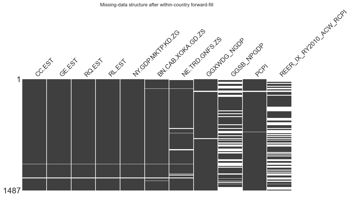

The results are quite revealing.

Forward-fill works well for variables whose missingness mainly reflects short interruptions within country series. Current account balance falls from 11.6% missing to 2.4%, trade openness from 13.1% to 5.3%, and the governance indicators plus GDP growth from about 9.4% to 1.3%. These reductions are substantial and support the idea that, for these variables, the most recent available observation is a reasonable proxy when a single year is missing.

By contrast, forward-fill does almost nothing for REER and structural fiscal balance. REER remains 42.7% missing and GGSB_NPGDP remains 34.2% missing. That is strong evidence that their missingness is not mainly due to short breaks within otherwise complete country series. It is structural.

One additional point needs to be made explicit. Forward-fill does not eliminate all missing values. For some country series, the first observed years are missing because there is no earlier value to carry forward. Those rows remain missing after forward-fill. That is expected. In other words, forward-fill can only repair interior gaps within a country sequence; it cannot create data for the beginning of a series where no prior observation exists.

Why not backward-fill? Backward-filling would use information from year $t+1$ or later to fill a missing value in year $t$. In a forecasting problem, that would violate the information set and would therefore constitute leakage. It is not acceptable here.

Missingness over time

Aggregate missingness rates are useful, but they do not reveal whether missing values are concentrated in particular periods. In a panel dataset, that is an important diagnostic. Missingness clustered in early years may reflect the gradual expansion of database coverage, while missingness that remains high throughout the sample is much more likely to reflect a structural problem.

To examine this, we compute the missing share of each variable by year.

missing_by_year_all = (
    panel_df.groupby("year")[candidate_features]
    .apply(lambda x: x.isna().mean())
)

plt.figure(figsize=(11, 5))

for col in candidate_features:
    plt.plot(
        missing_by_year_all.index,
        missing_by_year_all[col],
        label=col
    )

plt.title("Share of Missing Values by Year")
plt.xlabel("Year")
plt.ylabel("Missing share")
plt.legend(bbox_to_anchor=(1.02, 1), loc="upper left")

plt.tight_layout()
plt.show()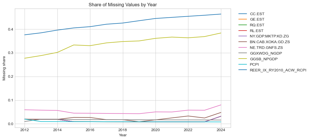

This figure reinforces the message from the matrix and the missingness table. Two variables dominate the profile throughout the sample: REER_IX_RY2010_ACW_RCPI and GGSB_NPGDP. Their missing shares are not just high in the early years; they remain very high across the whole panel. That makes them difficult to justify in a baseline forecasting model because their inclusion would sharply reduce the effective sample.

Once these structurally sparse variables are set aside, the remaining pattern becomes easier to interpret.

zoom_features = list(set(candidate_features) - set([
    "REER_IX_RY2010_ACW_RCPI",
    "GGSB_NPGDP"
]))

missing_by_year_zoom = (
    panel_df.groupby("year")[zoom_features]
    .apply(lambda x: x.isna().mean())
)

plt.figure(figsize=(11, 5))

for col in zoom_features:
    plt.plot(
        missing_by_year_zoom.index,
        missing_by_year_zoom[col],
        label=col
    )

plt.title("Share of Missing Values by Year (excluding structurally sparse variables)")
plt.xlabel("Year")
plt.ylabel("Missing share")
plt.legend(bbox_to_anchor=(1.02, 1), loc="upper left")

plt.tight_layout()
plt.show()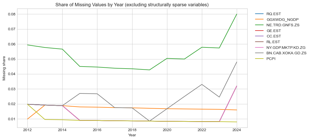

This second plot shows that the remaining variables are much more manageable. Several points stand out.

First, trade openness (NE.TRD.GNFS.ZS) remains the least complete among the retained variables, fluctuating around 4–8% missing depending on the year. That is not negligible, but it is still far below the structural sparsity seen in REER and structural balance.

Second, current account balance (BN.CAB.XOKA.GD.ZS) is more stable, generally in the low single digits, though it worsens somewhat toward the end of the sample.

Third, the governance indicators and GDP growth become very complete after forward-fill, typically around 1–2% missing, before rising slightly in 2024. That late increase is economically plausible: the final year of a panel is often the least complete because international databases update with a lag.

Fourth, PCPI and government debt remain among the most complete series throughout.

Overall, the time profile clarifies the nature of the missing-data problem. The difficulty is not that the whole panel is badly incomplete. Rather, it is that a small number of variables suffer from persistent structural sparsity, while the rest are reasonably usable once the panel structure is exploited.

Final missing data strategy

The missing-data strategy follows two principles:

preserve the time-series structure of the panel
avoid introducing information that would not have been available at the time of prediction

The resulting approach is deliberately simple and transparent.

Step 1: Forward-fill within country

Because many missing observations represent short interruptions within country time series, we use within-country forward-fill to propagate the most recent available observation.

panel_df = model_df.sort_values(["country_clean", "year"]).copy()

panel_df[candidate_features] = (
    panel_df.groupby("country_clean")[candidate_features]
    .ffill()
)

This is appropriate for macroeconomic and institutional indicators that evolve gradually over time. It does not create information from the future and therefore remains compatible with the forecasting design.

Step 2: Excluding structurally sparse variables

The missingness diagnostics support excluding two variables from the baseline modelling pool:

REER_IX_RY2010_ACW_RCPI
GGSB_NPGDP

Both remain heavily incomplete even after forward-fill, with missing shares of 42.7% and 34.2% respectively. Their omission should not be interpreted as a claim that exchange-rate competitiveness or structural fiscal balance are economically unimportant. Rather, it is a data-quality decision: including them would dramatically reduce the effective sample and would make the baseline model much less robust.

Step 3: Constructing the usable feature pool

Once these structurally sparse variables are excluded, the remaining variables form the usable pool from which the final modelling features will be selected.

Even after within-country forward-fill, a small amount of missingness remains. This is expected. Forward-fill can only propagate the most recent earlier value within the same country, so it cannot fill leading-edge gaps at the start of a country’s series, when no prior observation exists yet. That pattern is visible in the missingness diagnostics above: after forward-fill, most of the remaining gaps are concentrated at the beginning of country panels rather than appearing as frequent interruptions throughout otherwise complete series. In other words, the remaining missing values mainly reflect country-years for which we still do not have any earlier country-specific information to carry forward.

Rather than applying a second-round imputation, we construct the final training and test pools using .dropna(). This is a conservative choice, but a defensible one in this setting.

First, once the most problematic variables have been removed and within-country forward-fill has been applied, the remaining missingness is limited enough that complete-case analysis preserves most of the sample.

Second, additional imputation would be harder to justify economically. If a value cannot be filled from earlier observations for the same country, the alternative would be to impute using information from other countries or from a global average. In a sovereign-risk setting, that is often not appropriate. Countries differ systematically in institutional quality, external vulnerability, debt tolerance, and inflation dynamics. Imputing a missing fiscal or governance value for one sovereign using the cross-country distribution would risk creating an artificial “average sovereign” that is not economically meaningful for that country. That is especially problematic when the goal is to predict a rating threshold that depends precisely on persistent country-specific characteristics.

So .dropna() is used here not because imputation is impossible, but because after the earlier missing-data steps it becomes the more transparent and defensible option. It avoids introducing synthetic country-year values that cannot be justified by the panel structure, while still leaving sufficiently large modelling samples. The resulting training and test pools therefore contain no missing values in the usable predictors.

# ------------------------------------------------------------
# Final usable feature pool after forward-fill and structural exclusions
# ------------------------------------------------------------
usable_features = [
    "CC.EST",
    "GE.EST",
    "RQ.EST",
    "RL.EST",
    "NY.GDP.MKTP.KD.ZG",
    "BN.CAB.XOKA.GD.ZS",
    "NE.TRD.GNFS.ZS",
    "GGXWDG_NGDP",
    "PCPI"
]

train_pool = panel_df.loc[
    panel_df["year"] <= 2019,
    usable_features + ["target_ig", "year", "country_clean", "is_ig"]
].dropna().copy()

test_pool = panel_df.loc[
    panel_df["year"] >= 2020,
    usable_features + ["target_ig", "year", "country_clean", "is_ig"]
].dropna().copy()

print(f"Final training pool: {len(train_pool)}")
print(f"Final test pool: {len(test_pool)}")
print("\nTraining-pool columns:")
print(train_pool.columns.tolist())

Final training pool: 819
Final test pool: 554

Training-pool columns:
['CC.EST', 'GE.EST', 'RQ.EST', 'RL.EST', 'NY.GDP.MKTP.KD.ZG', 'BN.CAB.XOKA.GD.ZS', 'NE.TRD.GNFS.ZS', 'GGXWDG_NGDP', 'PCPI', 'target_ig', 'year', 'country_clean', 'is_ig']

These pool sizes are important. Relative to the original split of 880 training and 607 test observations, the remaining missing values after forward-fill lead to only a moderate loss of sample. That is a defensible trade-off: the model retains most of the panel while avoiding variables whose inclusion would have imposed much sharper losses, and the final modelling pools are fully observed on the retained predictors.

Feature selection strategy

Feature selection is not driven by a single rule. Instead, it combines four considerations:

Coverage and sample preservation Variables with severe structural missingness are excluded first because including them would sharply reduce the usable panel.
Economic relevance to sovereign credit risk The final set should span the main channels through which sovereign ratings are determined: institutional quality, fiscal sustainability, and external vulnerability.
Incremental information content A variable is not retained just because it is available. It should add something not already well captured by the others.
Stability and interpretability in a parametric model Because the baseline model is logistic regression, heavily collinear predictors are a problem.

A particularly important issue arises among the governance indicators.

gov_cols = ['CC.EST', 'GE.EST', 'RQ.EST', 'RL.EST']
print("Governance indicator inter-correlations (training pool):")
print(train_pool[gov_cols].corr().round(3).to_string())

Governance indicator inter-correlations (training set):
        CC.EST  GE.EST  RQ.EST  RL.EST
CC.EST   1.000   0.936   0.894   0.955
GE.EST   0.936   1.000   0.936   0.956
RQ.EST   0.894   0.936   1.000   0.932
RL.EST   0.955   0.956   0.932   1.000

These correlations are extremely high. All pairwise relationships exceed 0.89, and the strongest are around 0.95–0.96. So although these variables represent distinct governance concepts in theory, in this sample they are moving very closely together. That creates an immediate modelling issue: including all of them simultaneously in logistic regression would make coefficient estimates unstable and hard to interpret.

It is also useful to examine the broader correlation structure across the full candidate pool.

print("Broader correlation matrix on the final training pool:")
print(train_pool[usable_features].corr().round(3).to_string())

Broader correlation matrix on the final training pool:
                   CC.EST  GE.EST  RQ.EST  RL.EST  NY.GDP.MKTP.KD.ZG  BN.CAB.XOKA.GD.ZS  NE.TRD.GNFS.ZS  GGXWDG_NGDP   PCPI
CC.EST              1.000   0.939   0.896   0.955             -0.056              0.307           0.372        0.155 -0.060
GE.EST              0.939   1.000   0.939   0.960             -0.044              0.376           0.406        0.165 -0.072
RQ.EST              0.896   0.939   1.000   0.938              0.001              0.334           0.401        0.074 -0.055
RL.EST              0.955   0.960   0.938   1.000             -0.027              0.338           0.385        0.155 -0.050
NY.GDP.MKTP.KD.ZG  -0.056  -0.044   0.001  -0.027              1.000             -0.072           0.048       -0.325 -0.079
BN.CAB.XOKA.GD.ZS   0.307   0.376   0.334   0.338             -0.072              1.000           0.203       -0.120 -0.022
NE.TRD.GNFS.ZS      0.372   0.406   0.401   0.385              0.048              0.203           1.000       -0.087 -0.107
GGXWDG_NGDP         0.155   0.165   0.074   0.155             -0.325             -0.120          -0.087        1.000  0.044
PCPI               -0.060  -0.072  -0.055  -0.050             -0.079             -0.022          -0.107        0.044  1.000

The broader correlation matrix helps contextualise the selection problem. Several patterns stand out.

First, the governance block is much more internally correlated than the rest of the feature set. This confirms that governance redundancy is the main multicollinearity issue.

Second, most macroeconomic variables are only moderately correlated with the governance indicators and with one another. That is useful because it suggests they may contribute information that is not simply a re-expression of institutional quality.

Third, some of the expected economic patterns are visible even at the correlation stage. For example, better governance is positively associated with stronger external balances and slightly positively associated with trade openness, while higher debt is negatively associated with GDP growth and weakly negatively associated with current account performance. These are not strong enough to force exclusion, but they do confirm that the variables are economically connected in plausible ways.

Economic rationale before formal selection

Before turning to a formal feature-selection procedure, it is helpful to state the economic logic of the candidate variables.

Governance indicators (CC.EST, GE.EST, RQ.EST, RL.EST) These are conceptually central because sovereign ratings reflect not only ability to repay but also willingness and capacity to govern effectively. Strong institutions support tax collection, policy credibility, debt management, and macroeconomic stability.
GDP growth (NY.GDP.MKTP.KD.ZG) Growth matters because a stronger economy supports debt sustainability and external repayment capacity. However, the earlier EDA suggested that growth is not a clean discriminator between IG and non-IG: some non-IG countries grow quickly, but from weaker institutional and fiscal starting points.
Current account balance (BN.CAB.XOKA.GD.ZS) This is economically important because persistent external deficits increase dependence on foreign capital inflows and raise vulnerability to sudden stops and refinancing pressure.
Trade openness (NE.TRD.GNFS.ZS) Openness captures integration into global trade networks. It may support sovereign creditworthiness through export capacity and external earnings, but it can also reflect the structure of small open economies, so its sign is not guaranteed ex ante.
Government debt (GGXWDG_NGDP) This is one of the most direct fiscal-sustainability indicators. Higher debt reduces fiscal flexibility and increases sensitivity to interest-rate shocks.
Price level variable (PCPI) The raw level of PCPI is difficult to compare across countries because it is not on a common cross-country scale in the way an inflation rate would be. So even though it remains relatively complete, its economic interpretation in this form is weaker than the other retained candidates.

This means feature selection is not just statistical housekeeping. It is a way of deciding which variables provide the cleanest and most defensible baseline representation of the three core dimensions of sovereign risk in this dataset: institutional quality, external vulnerability, and fiscal sustainability.

Sequential Forward Selection (SFS)

To avoid making the final feature set look purely ad hoc, the economic screening above is combined with Sequential Forward Selection (SFS) under a time-aware cross-validation structure.

The idea is simple: once the obviously unusable variables have been removed, SFS adds predictors one at a time, each time choosing the variable that improves cross-validated performance the most. Because this is a forecasting problem, the selection procedure must also respect the temporal structure of the data.

The next code blocks first construct an expanding-window cross-validation design and then visualise it.

train_pool_sorted = train_pool.sort_values(["year", "country_clean"]).reset_index(drop=True)

X_train_fs = train_pool_sorted[usable_features]
y_train_fs = train_pool_sorted["target_ig"]

tscv = TimeSeriesSplit(n_splits=5)
cv_splits = list(tscv.split(X_train_fs))

fig, ax = plt.subplots(figsize=(10, 4))

for i, (train_idx, val_idx) in enumerate(cv_splits):
    train_years = sorted(train_pool_sorted.loc[train_idx, "year"].unique())
    val_years   = sorted(train_pool_sorted.loc[val_idx, "year"].unique())

    ax.barh(
        i,
        max(train_years) - min(train_years) + 1,
        left=min(train_years),
        height=0.4,
        color="tab:blue",
        label="Train" if i == 0 else None
    )

    ax.barh(
        i,
        max(val_years) - min(val_years) + 1,
        left=min(val_years),
        height=0.4,
        color="tab:orange",
        label="Validation" if i == 0 else None
    )

ax.set_yticks(range(len(cv_splits)))
ax.set_yticklabels([f"Fold {i+1}" for i in range(len(cv_splits))])
ax.set_xlabel("Year")
ax.set_title("Expanding-window cross-validation for feature selection")
ax.legend(loc="upper center", bbox_to_anchor=(0.5, -0.15), ncol=2, frameon=False)

plt.tight_layout()
plt.show()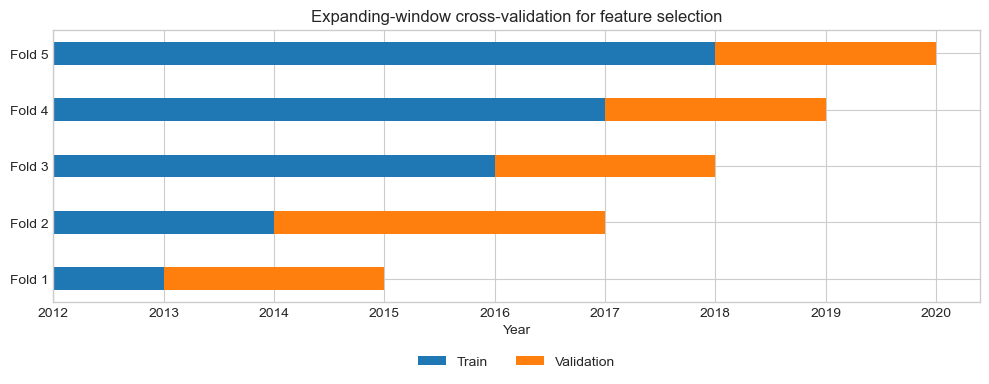

This expanding-window design is important. Each validation block occurs after its corresponding training block, so the feature-selection procedure respects the forecasting logic of the problem. That is especially relevant in a sovereign panel, where the economic environment changes over time and later observations should not be allowed to influence earlier validation periods.

Now apply SFS using logistic regression as the base classifier.

logit_sfs_pipe = Pipeline([
    ("scaler", StandardScaler()),
    ("model", LogisticRegression(
        max_iter=1000,
        class_weight="balanced",
        random_state=42
    ))
])

sfs = SequentialFeatureSelector(
    logit_sfs_pipe,
    n_features_to_select=6,
    direction="forward",
    scoring="balanced_accuracy",
    cv=tscv,
    n_jobs=-1
)

sfs.fit(X_train_fs, y_train_fs)

selected_features = X_train_fs.columns[sfs.get_support()]
print("Selected features:", list(selected_features))

Selected features: ['CC.EST', 'GE.EST', 'RQ.EST', 'BN.CAB.XOKA.GD.ZS', 'NE.TRD.GNFS.ZS', 'GGXWDG_NGDP']

This result is both statistically and economically coherent.

From a statistical perspective, SFS does not select GDP growth, PCPI, or rule of law. That suggests these variables add little incremental predictive information once the selected set is already in the model.

From an economic perspective, the selected variables span exactly the three dimensions that sovereign rating analysis would normally emphasise:

institutional quality: CC.EST, GE.EST, RQ.EST
external vulnerability / external strength: BN.CAB.XOKA.GD.ZS, NE.TRD.GNFS.ZS
fiscal sustainability: GGXWDG_NGDP

The omission of RL.EST is easy to justify given the extreme correlations in the governance block: its information is already largely absorbed by the three governance indicators that remain. The omission of GDP growth is also economically plausible. Growth matters, but in this panel it is a relatively weak discriminator between IG and non-IG once governance, external balance, and debt are already accounted for. The omission of PCPI is also sensible because the raw price level is not the cleanest cross-country macro signal in this setting.

Final feature set for modelling

Using the missing-data diagnostics, the economic screening, and the SFS results together, we define the final modelling feature set.

sov_features = list(selected_features)
print("Final modelling features:", sov_features)

Final modelling features: ['CC.EST', 'GE.EST', 'RQ.EST', 'BN.CAB.XOKA.GD.ZS', 'NE.TRD.GNFS.ZS', 'GGXWDG_NGDP']

These final predictors form a parsimonious but economically meaningful baseline feature set.

The three governance variables capture the idea that sovereign creditworthiness depends not only on raw macro indicators, but also on the quality of institutions that manage fiscal policy, regulate the economy, and sustain policy credibility. The current-account balance and trade openness capture external vulnerability and international integration, both of which matter for a sovereign’s ability to withstand tightening global financial conditions. Government debt captures fiscal sustainability, a central component of any sovereign rating assessment.

So the final set is intentionally selective rather than exhaustive. The goal is not to include every available variable, but to build a baseline model that is:

economically interpretable
supported by time-aware empirical selection
robust to missingness
not overwhelmed by multicollinearity
broad enough to cover the main channels of sovereign credit risk in this dataset.

With the feature set now fixed, the next step is to estimate the actual models and ask what, if anything, they add beyond the persistence baseline.

The selected features are then extracted from the complete-case training and test pools constructed above. At this point, the modelling datasets contain no missing values in either the predictors or the target, so no further imputation is required before estimation.

# Final modelling datasets based on the selected features
train_clean = train_pool[sov_features + ["target_ig", "country_clean", "year", "is_ig"]].copy()
test_clean  = test_pool[sov_features + ["target_ig", "country_clean", "year", "is_ig"]].copy()

print(f"Final training sample: {len(train_clean)}")
print(f"Final test sample: {len(test_clean)}")

X_train = train_clean[sov_features]
y_train = train_clean["target_ig"]

X_test = test_clean[sov_features]
y_test = test_clean["target_ig"]

Final training sample: 819
Final test sample: 554

These final modelling samples are large enough to support meaningful estimation and evaluation, while remaining fully observed on the retained predictors. That matters because it allows the modelling exercise to proceed without introducing additional synthetic values for country-years where no defensible country-specific information is available.

Q2.4.3: Baseline logistic regression (Macro Variables Only)

The first model is a logistic regression classifier estimated using only the selected macroeconomic and institutional variables:

CC.EST
GE.EST
RQ.EST
BN.CAB.XOKA.GD.ZS
NE.TRD.GNFS.ZS
GGXWDG_NGDP

This is the natural baseline for two reasons.

First, the target variable is binary: whether the sovereign is investment grade in year (t+1).

Second, logistic regression is transparent. In a dataset where persistence is overwhelmingly strong, transparency is particularly valuable because it allows us to separate two different questions:

structural interpretation: which macroeconomic and governance characteristics are associated with IG status?
predictive performance: does the model add anything beyond the persistence rule?

The baseline logistic model is designed to answer the first question most directly. It deliberately does not include the current IG label as a predictor, because the purpose here is to see how far the macro and institutional data can go on their own.

Why standardise the predictors?

The retained predictors are measured on very different scales. Governance indicators vary roughly between −2.5 and +2.5, current-account balances are percentages of GDP, and debt ratios can exceed 100% of GDP. Standardising the predictors places them on a common scale, so the coefficients can be interpreted as the effect of a one-standard-deviation increase in each variable.

Why use balanced class weights?

The main problem in this dataset is not a classic cross-sectional imbalance between IG and non-IG. Rather, it is the extreme persistence of the target through time. Using class_weight='balanced' is therefore a conservative way to ensure that both classes contribute symmetrically to the fitted objective rather than letting the optimisation lean too heavily toward the dominant empirical pattern of “no change”.

The next block fits the baseline model.

scaler = StandardScaler()
X_train_sc = scaler.fit_transform(X_train)
X_test_sc  = scaler.transform(X_test)

logit = LogisticRegression(
    max_iter=1000,
    class_weight="balanced",
    random_state=42
)

logit.fit(X_train_sc, y_train)

Why these evaluation metrics?

The evaluation metrics are chosen to reflect the structure of the dataset and the economics of the problem.

Balanced accuracy is the main threshold-based metric because it gives equal weight to the IG and non-IG classes. That matters because a model should not look good simply because it predicts the more common class well. However, balanced accuracy does not solve the persistence problem by itself. As Section 2.4.1 showed, the persistence rule still achieves almost perfect balanced accuracy because threshold crossings are so rare.

Macro F1 complements balanced accuracy by incorporating both precision and recall for each class. This is useful because the two types of classification error have different meanings. A false positive predicts IG for a sovereign that is actually non-IG, which is the more dangerous mistake for an investor or lender. A false negative predicts non-IG for a sovereign that is actually IG, which is a more conservative mistake.

ROC-AUC is especially important in this dataset because it evaluates the model’s ranking ability across all thresholds. That matters because one plausible use of a macro-based model here is not necessarily to beat persistence on hard 0/1 classifications, but to identify which sovereigns lie closest to the boundary and therefore merit closer attention.

PR-AUC is also useful because it tells us whether the model is concentrating predicted probability mass in a meaningful way. In a setting where the economically important cases are rare and threshold-based accuracy is dominated by persistence, PR-AUC provides another view of whether the model is learning a useful probability signal rather than just reproducing the broad class structure.

The next block computes these metrics on both the training and test sets.

y_train_pred = logit.predict(X_train_sc)
y_train_prob = logit.predict_proba(X_train_sc)[:, 1]

y_test_pred = logit.predict(X_test_sc)
y_test_prob = logit.predict_proba(X_test_sc)[:, 1]

for y_true, y_pred, y_prob, label in [
    (y_train, y_train_pred, y_train_prob, "Train"),
    (y_test,  y_test_pred,  y_test_prob,  "Test")
]:
    print(f"\n{label}:")
    print(f"  Balanced Accuracy: {balanced_accuracy_score(y_true, y_pred):.4f}")
    print(f"  Macro F1:          {f1_score(y_true, y_pred, average='macro'):.4f}")
    print(f"  ROC-AUC:           {roc_auc_score(y_true, y_prob):.4f}")
    print(f"  PR-AUC:            {average_precision_score(y_true, y_prob):.4f}")

Train:
  Balanced Accuracy: 0.8894
  Macro F1:          0.8895
  ROC-AUC:           0.9604
  PR-AUC:            0.9692

Test:
  Balanced Accuracy: 0.8681
  Macro F1:          0.8680
  ROC-AUC:           0.9425
  PR-AUC:            0.9389

To make the classification errors easier to interpret, we also inspect the confusion matrices.

fig, axes = plt.subplots(1, 2, figsize=(10, 4))

for ax, y_true, y_pred, y_prob, label in [
    (axes[0], y_train, y_train_pred, y_train_prob, "Training"),
    (axes[1], y_test,  y_test_pred,  y_test_prob,  "Test")
]:
    cm = confusion_matrix(y_true, y_pred)
    sns.heatmap(cm, annot=True, fmt="d", cmap="Blues", cbar=False, ax=ax)
    ax.set_xlabel("Predicted")
    ax.set_ylabel("Actual")
    ax.set_title(
        f"Logistic Regression: {label}\n"
        f"BalAcc={balanced_accuracy_score(y_true, y_pred):.3f}, "
        f"ROC-AUC={roc_auc_score(y_true, y_prob):.3f}",
        fontsize=10
    )

plt.tight_layout()
plt.show()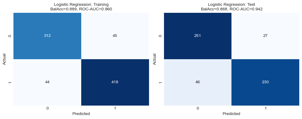

The confusion matrices show that the model performs reasonably symmetrically across the two classes, but it still makes a non-trivial number of mistakes on both sides of the boundary. In the test set, it correctly classifies 251 non-IG and 230 IG observations, but still produces 27 false positives and 46 false negatives. So the model is not simply collapsing into one class; it is genuinely attempting to distinguish the two groups.

Cross-validation performance

A single train/test split is useful, but not sufficient. Because the dataset spans several different macro-financial environments, it is important to check whether performance is stable across different historical windows within the training sample.

The next block evaluates the macro-only logistic model under the same expanding-window time-series cross-validation structure used earlier for feature selection.

cv_logit_macro = cross_validate(
    logit,
    X_train_sc,
    y_train,
    cv=tscv,
    scoring={
        "balanced_accuracy": "balanced_accuracy",
        "macro_f1": "f1_macro",
        "roc_auc": "roc_auc",
        "pr_auc": "average_precision"
    },
    n_jobs=-1
)

cv_logit_macro_df = pd.DataFrame({
    "fold": range(1, len(cv_logit_macro["test_balanced_accuracy"]) + 1),
    "balanced_accuracy": cv_logit_macro["test_balanced_accuracy"],
    "macro_f1": cv_logit_macro["test_macro_f1"],
    "roc_auc": cv_logit_macro["test_roc_auc"],
    "pr_auc": cv_logit_macro["test_pr_auc"]
})

print(cv_logit_macro_df.round(4).to_string(index=False))

cv_logit_macro_summary = pd.DataFrame({
    "Model": ["Logistic (macro only)"],
    "CV Balanced Accuracy": [cv_logit_macro_df["balanced_accuracy"].mean()],
    "CV Macro F1": [cv_logit_macro_df["macro_f1"].mean()],
    "CV ROC-AUC": [cv_logit_macro_df["roc_auc"].mean()],
    "CV PR-AUC": [cv_logit_macro_df["pr_auc"].mean()],
    "CV Balanced Accuracy SD": [cv_logit_macro_df["balanced_accuracy"].std()],
    "CV Macro F1 SD": [cv_logit_macro_df["macro_f1"].std()],
    "CV ROC-AUC SD": [cv_logit_macro_df["roc_auc"].std()],
    "CV PR-AUC SD": [cv_logit_macro_df["pr_auc"].std()]
})

print(cv_logit_macro_summary.round(4).to_string(index=False))

 fold  balanced_accuracy  macro_f1  roc_auc  pr_auc
    1             0.7212    0.7200   0.8821  0.8907
    2             0.8160    0.7612   0.9453  0.9758
    3             0.9016    0.8894   0.9679  0.9787
    4             0.8734    0.8577   0.9413  0.9574
    5             0.9272    0.9262   0.9902  0.9917

                Model  CV Balanced Accuracy  CV Macro F1  CV ROC-AUC  CV PR-AUC  CV Balanced Accuracy SD  CV Macro F1 SD  CV ROC-AUC SD  CV PR-AUC SD
Logistic (macro only)                0.8479       0.8309      0.9454     0.9588                    0.082          0.0871         0.0404          0.04

These cross-validation results add important nuance.

The fold-level metrics vary materially, especially for the threshold-based measures. Balanced accuracy ranges from 0.7212 in the weakest fold to 0.9272 in the strongest, and macro F1 ranges from 0.7200 to 0.9262. That tells us the macro-only logistic model does not deliver equally strong threshold-based classification performance in every historical window.

The ranking metrics are more stable in relative terms, though not identical across folds. ROC-AUC ranges from 0.8821 to 0.9902, and PR-AUC from 0.8907 to 0.9917. So even here there is real time variation, but the model’s ability to order sovereigns by relative IG likelihood appears more consistent than its exact 0/1 classification performance.

Three comparisons matter.

Train vs test

The train–test gaps are modest:

balanced accuracy: 0.8894 → 0.8681 (gap = −0.0213)
macro F1: 0.8895 → 0.8680 (gap = −0.0215)
ROC-AUC: 0.9604 → 0.9425 (gap = −0.0179)
PR-AUC: 0.9692 → 0.9389 (gap = −0.0303)

These are small enough to suggest that the model is not strongly overfitting the final training sample.

CV vs train

The CV–train gaps are larger:

balanced accuracy: 0.8479 vs 0.8894 (gap = −0.0415)
macro F1: 0.8309 vs 0.8895 (gap = −0.0586)
ROC-AUC: 0.9454 vs 0.9604 (gap = −0.0150)
PR-AUC: 0.9588 vs 0.9692 (gap = −0.0104)

That suggests the model looks somewhat stronger when fitted on the full training window than when repeatedly estimated on smaller expanding samples. Economically, that is plausible: the more historical sovereign environments the model sees, the easier it becomes to estimate a stable linear separation between stronger and weaker credit profiles.

CV vs test

The CV–test comparison is actually reassuring:

balanced accuracy: 0.8479 vs 0.8681 (test higher by +0.0202)
macro F1: 0.8309 vs 0.8680 (test higher by +0.0371)
ROC-AUC: 0.9454 vs 0.9425 (difference = −0.0029)
PR-AUC: 0.9588 vs 0.9389 (difference = −0.0199)

So the final holdout test set is not inconsistent with the cross-validation evidence. In particular, the ROC-AUC is extremely close between CV mean and final test. That is strong evidence that the model’s ranking ability is more stable than its exact threshold performance.

A careful summary is therefore:

The macro-only logistic regression does not beat persistence on threshold-based metrics, and its balanced accuracy varies across folds. But it shows limited train–test degradation, which argues against severe overfitting, and its CV and final test ROC-AUC are almost identical. So the model is better viewed as a tool for ranking sovereigns by relative IG likelihood than as a fully stable hard-classification rule.

Comparison with the persistence benchmark

It is useful to compare the baseline logistic regression directly with persistence.

comparison_baseline_train = pd.DataFrame({
    "Model": ["Persistence rule", "Logistic (macro only)"],
    "Balanced Accuracy": [
        balanced_accuracy_score(y_true_bench_train, y_pred_persist_train),
        balanced_accuracy_score(y_train, y_train_pred)
    ],
    "Macro F1": [
        f1_score(y_true_bench_train, y_pred_persist_train, average="macro"),
        f1_score(y_train, y_train_pred, average="macro")
    ],
    "ROC-AUC": [np.nan, roc_auc_score(y_train, y_train_prob)],
    "PR-AUC": [np.nan, average_precision_score(y_train, y_train_prob)]
})

comparison_baseline_test = pd.DataFrame({
    "Model": ["Persistence rule", "Logistic (macro only)"],
    "Balanced Accuracy": [
        balanced_accuracy_score(y_true_bench_test, y_pred_persist_test),
        balanced_accuracy_score(y_test, y_test_pred)
    ],
    "Macro F1": [
        f1_score(y_true_bench_test, y_pred_persist_test, average="macro"),
        f1_score(y_test, y_test_pred, average="macro")
    ],
    "ROC-AUC": [np.nan, roc_auc_score(y_test, y_test_prob)],
    "PR-AUC": [np.nan, average_precision_score(y_test, y_test_prob)]
})

print("Training comparison:")
print(comparison_baseline_train.round(4).to_string(index=False))

print("\nTest comparison:")
print(comparison_baseline_test.round(4).to_string(index=False))

Training comparison:
                Model  Balanced Accuracy  Macro F1  ROC-AUC  PR-AUC
     Persistence rule             0.9796    0.9803      NaN     NaN
Logistic (macro only)             0.8894    0.8895   0.9604  0.9692

Test comparison:
                Model  Balanced Accuracy  Macro F1  ROC-AUC  PR-AUC
     Persistence rule             0.9918    0.9918      NaN     NaN
Logistic (macro only)             0.8681    0.8680   0.9425  0.9389

This comparison is the key interpretive discipline for the rest of the section.

On hard class labels, the macro-only logistic regression is well below persistence. That is not a failure of estimation. It is a reflection of the data-generating environment: the persistence rule is exploiting the strongest empirical regularity in the dataset, namely that sovereign IG status almost always remains unchanged from one year to the next.

So the macro-only model should not be judged mainly on whether it beats persistence on balanced accuracy or macro F1. Instead, its value lies in two narrower but still important roles:

it provides a probability ranking through ROC-AUC and PR-AUC;
it yields interpretable coefficients on the macro and governance variables.

Distribution of predicted probabilities

Because ranking is central here, it is useful to inspect the distribution of predicted IG probabilities in the test set.

plt.figure(figsize=(8, 4))
plt.hist(y_test_prob, bins=30, alpha=0.75)
plt.axvline(0.5, color="red", linestyle="--", label="Decision threshold")
plt.title("Distribution of predicted IG probabilities (macro-only logistic regression)")
plt.xlabel("Predicted probability of investment grade")
plt.ylabel("Frequency")
plt.legend()
plt.tight_layout()
plt.show()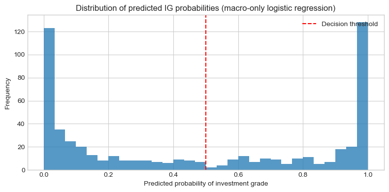

The probability distribution is strongly bimodal. Many observations are assigned probabilities very close to 0 or very close to 1, while a smaller middle mass lies around the threshold region. This is exactly what one would expect in a sovereign-rating context. Most sovereigns are clearly deep inside one regime or the other; the economically interesting cases are the smaller set of borderline sovereigns whose macro and institutional indicators place them close to the BBB− / BB+ boundary.

Coefficient interpretation

The main advantage of the baseline logistic model is interpretability.

coef_table = pd.DataFrame({
    "Feature": sov_features,
    "Coefficient": logit.coef_[0]
})

coef_table["Odds_Ratio"] = np.exp(coef_table["Coefficient"])
coef_table = coef_table.sort_values("Coefficient", ascending=False)

print(coef_table.round(4).to_string(index=False))

          Feature  Coefficient  Odds_Ratio
           GE.EST       3.1593     23.5546
           RQ.EST       2.2748      9.7257
BN.CAB.XOKA.GD.ZS       1.3379      3.8112
   NE.TRD.GNFS.ZS      -1.1141      0.3282
      GGXWDG_NGDP      -1.1614      0.3131
           CC.EST      -1.5992      0.2021

Because the predictors are standardised, the coefficients are directly comparable. A positive coefficient means that a one-standard-deviation increase in the variable is associated with a higher probability of next-year IG status, holding the other predictors fixed. A negative coefficient means the opposite.

The results are economically informative.

GE.EST is by far the strongest positive predictor. A one-standard-deviation increase in government effectiveness multiplies the odds of next-year IG status by about 23.6 times. That is a very large effect, but also a plausible one. Sovereign ratings do not only measure a country’s current macro position; they also reflect whether the state is capable of implementing policy, collecting revenue, managing debt, and reacting credibly to shocks. In sovereign-risk terms, government effectiveness captures both capacity to repay and, indirectly, the credibility of the policy framework supporting that repayment.

RQ.EST is also strongly positive, with an odds ratio of about 9.7. This reinforces the same broader message: sovereign creditworthiness is not determined by fiscal ratios alone. Rating agencies place substantial weight on policy quality and institutional credibility because these shape how countries respond when stress arrives.

BN.CAB.XOKA.GD.ZS is positive as expected. A stronger current-account balance multiplies the odds of IG by about 3.8 per standard deviation. That is economically intuitive. Countries with more favourable external balances are less dependent on foreign capital inflows and less vulnerable to sudden-stop dynamics when global financial conditions tighten.

GGXWDG_NGDP is negative, also as expected. A one-standard-deviation increase in government debt reduces the odds of IG to about 31% of their previous level. That is the classic fiscal-sustainability channel: higher debt reduces fiscal flexibility and increases vulnerability to financing shocks and interest-rate increases.

Two coefficients require more care.

NE.TRD.GNFS.ZS is negative. This is not a claim that trade openness is harmful in itself. It is a conditional multivariate effect. In this dataset, some highly open economies are small emerging or frontier sovereigns that remain non-IG despite being very integrated into trade. Once governance, current account balance, and debt are already controlled for, openness by itself is not functioning as a clean positive IG signal.

CC.EST is also negative, despite the strong positive bivariate separation seen earlier in the EDA. This is best understood as a multicollinearity effect. The governance indicators are extremely highly correlated, so once GE.EST and RQ.EST are already in the model, CC.EST is being interpreted conditionally on those other governance dimensions. This does not mean corruption control is irrelevant. It means that in this particular multivariate specification, much of its positive governance signal is already absorbed by the other governance indicators.

So the substantive conclusion from the baseline model is clear:

The macro-only logistic regression suggests that institutional quality, especially government effectiveness and regulatory quality, is the dominant structural separator between IG and non-IG sovereigns in this dataset. External balance and public debt also matter in economically plausible directions. The model is therefore useful primarily as a structural interpretation tool and as a probability-ranking model, not as a replacement for the persistence rule on hard classifications.

Q2.4.4: Logistic regression with current IG status added

The next step is to add the current-year IG label itself as a predictor.

This model addresses a sharper empirical question than the macro-only baseline:

Once current IG status is explicitly included, do the macroeconomic and governance variables add anything beyond persistence?

This is an important test because the macro-only model may partly be using governance and macro variables to proxy for current class membership. Strong-governance sovereigns tend to remain IG; weak-governance sovereigns tend to remain non-IG. If so, some of the apparent explanatory power of the macro-only model is really just persistence operating indirectly through macro and institutional variables.

Adding the current IG status separates these two channels more cleanly.

There is also an important technical point to make explicit. Including the current IG label does not create perfect separation in the strict econometric sense. If it did, the model would classify the target without error and the logistic coefficients would diverge. But that does not happen here, because there are still genuine transition cases in which current IG differs from next-year IG. So the model becomes much more predictive, but not perfectly deterministic.

The following code fits the augmented logistic model.

train_clean_v2 = train_clean.copy()
test_clean_v2  = test_clean.copy()

train_clean_v2["is_ig_current"] = train_clean_v2["is_ig"]
test_clean_v2["is_ig_current"]  = test_clean_v2["is_ig"]

sov_features_v2 = sov_features + ["is_ig_current"]

X_train_v2 = train_clean_v2[sov_features_v2]
y_train_v2 = train_clean_v2["target_ig"]

X_test_v2 = test_clean_v2[sov_features_v2]
y_test_v2 = test_clean_v2["target_ig"]

scaler_v2 = StandardScaler()
X_train_v2_sc = scaler_v2.fit_transform(X_train_v2)
X_test_v2_sc  = scaler_v2.transform(X_test_v2)

logit_v2 = LogisticRegression(
    max_iter=1000,
    class_weight="balanced",
    random_state=42
)

logit_v2.fit(X_train_v2_sc, y_train_v2)

Now evaluate it using the same metrics.

y_train_pred_v2 = logit_v2.predict(X_train_v2_sc)
y_train_prob_v2 = logit_v2.predict_proba(X_train_v2_sc)[:, 1]

y_test_pred_v2 = logit_v2.predict(X_test_v2_sc)
y_test_prob_v2 = logit_v2.predict_proba(X_test_v2_sc)[:, 1]

for y_true, y_pred, y_prob, label in [
    (y_train_v2, y_train_pred_v2, y_train_prob_v2, "Train"),
    (y_test_v2,  y_test_pred_v2,  y_test_prob_v2,  "Test")
]:
    print(f"\n{label} (macro + current IG):")
    print(f"  Balanced Accuracy: {balanced_accuracy_score(y_true, y_pred):.4f}")
    print(f"  Macro F1:          {f1_score(y_true, y_pred, average='macro'):.4f}")
    print(f"  ROC-AUC:           {roc_auc_score(y_true, y_prob):.4f}")
    print(f"  PR-AUC:            {average_precision_score(y_true, y_prob):.4f}")

Train (macro + current IG):
  Balanced Accuracy: 0.9781
  Macro F1:          0.9789
  ROC-AUC:           0.9949
  PR-AUC:            0.9956

Test (macro + current IG):
  Balanced Accuracy: 0.9892
  Macro F1:          0.9892
  ROC-AUC:           0.9960
  PR-AUC:            0.9966

To make the near-boundary mistakes easier to inspect, it is also useful to look at the confusion matrices.

fig, axes = plt.subplots(1, 2, figsize=(10, 4))

for ax, y_true, y_pred, y_prob, label in [
    (axes[0], y_train_v2, y_train_pred_v2, y_train_prob_v2, "Training"),
    (axes[1], y_test_v2,  y_test_pred_v2,  y_test_prob_v2,  "Test")
]:
    cm = confusion_matrix(y_true, y_pred)
    sns.heatmap(cm, annot=True, fmt="d", cmap="Blues", cbar=False, ax=ax)
    ax.set_xlabel("Predicted")
    ax.set_ylabel("Actual")
    ax.set_title(
        f"Logistic Regression + current IG: {label}\n"
        f"BalAcc={balanced_accuracy_score(y_true, y_pred):.3f}, "
        f"ROC-AUC={roc_auc_score(y_true, y_prob):.3f}",
        fontsize=10
    )

plt.tight_layout()
plt.show()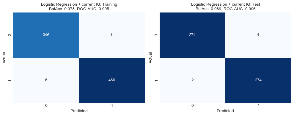

The confusion matrices make the effect of adding current IG immediately visible. In the test set, the model now makes only 6 mistakes in total: 4 false positives and 2 false negatives. That is dramatically better than the macro-only logistic regression, which made 73 mistakes in total on the same holdout sample.

Cross-validation performance

The augmented logistic model also needs to be checked across time windows.

cv_logit_full = cross_validate(
    logit_v2,
    X_train_v2_sc,
    y_train_v2,
    cv=tscv,
    scoring={
        "balanced_accuracy": "balanced_accuracy",
        "macro_f1": "f1_macro",
        "roc_auc": "roc_auc",
        "pr_auc": "average_precision"
    },
    n_jobs=-1
)

cv_logit_full_df = pd.DataFrame({
    "fold": range(1, len(cv_logit_full["test_balanced_accuracy"]) + 1),
    "balanced_accuracy": cv_logit_full["test_balanced_accuracy"],
    "macro_f1": cv_logit_full["test_macro_f1"],
    "roc_auc": cv_logit_full["test_roc_auc"],
    "pr_auc": cv_logit_full["test_pr_auc"]
})

print(cv_logit_full_df.round(4).to_string(index=False))

cv_logit_full_summary = pd.DataFrame({
    "Model": ["Logistic (macro + current IG)"],
    "CV Balanced Accuracy": [cv_logit_full_df["balanced_accuracy"].mean()],
    "CV Macro F1": [cv_logit_full_df["macro_f1"].mean()],
    "CV ROC-AUC": [cv_logit_full_df["roc_auc"].mean()],
    "CV PR-AUC": [cv_logit_full_df["pr_auc"].mean()],
    "CV Balanced Accuracy SD": [cv_logit_full_df["balanced_accuracy"].std()],
    "CV Macro F1 SD": [cv_logit_full_df["macro_f1"].std()],
    "CV ROC-AUC SD": [cv_logit_full_df["roc_auc"].std()],
    "CV PR-AUC SD": [cv_logit_full_df["pr_auc"].std()]
})

print(cv_logit_full_summary.round(4).to_string(index=False))

 fold  balanced_accuracy  macro_f1  roc_auc  pr_auc
    1             0.9773    0.9778   0.9870  0.9868
    2             0.9947    0.9913   0.9995  0.9998
    3             0.9741    0.9773   0.9956  0.9966
    4             0.9780    0.9755   0.9850  0.9888
    5             0.9773    0.9778   0.9976  0.9980

                        Model  CV Balanced Accuracy  CV Macro F1  CV ROC-AUC  CV PR-AUC  CV Balanced Accuracy SD  CV Macro F1 SD  CV ROC-AUC SD  CV PR-AUC SD
Logistic (macro + current IG)                0.9803       0.9799      0.9929      0.994                   0.0082          0.0064         0.0065        0.0058

These results are striking. Once current IG is added, performance becomes not only much stronger on average but also much more stable across historical windows. The fold dispersion is tiny compared with the macro-only model.

The gap structure confirms this.

Train vs test

balanced accuracy: 0.9781 → 0.9892 (test higher by +0.0111)
macro F1: 0.9789 → 0.9892 (test higher by +0.0103)
ROC-AUC: 0.9949 → 0.9960 (difference = +0.0011)
PR-AUC: 0.9956 → 0.9966 (difference = +0.0010)

There is effectively no sign of overfitting here.

CV vs train

balanced accuracy: 0.9803 vs 0.9781 (difference = +0.0022)
macro F1: 0.9799 vs 0.9789 (difference = +0.0010)
ROC-AUC: 0.9929 vs 0.9949 (difference = −0.0020)
PR-AUC: 0.9940 vs 0.9956 (difference = −0.0016)

CV vs test

balanced accuracy: 0.9803 vs 0.9892 (difference = +0.0089)
macro F1: 0.9799 vs 0.9892 (difference = +0.0093)
ROC-AUC: 0.9929 vs 0.9960 (difference = +0.0031)
PR-AUC: 0.9940 vs 0.9966 (difference = +0.0026)

So unlike the macro-only model, the augmented logistic specification is extremely consistent across train, CV, and test.

Comparison with the baseline logistic model

comparison_logit = pd.DataFrame({
    "Model": [
        "Logistic (macro only)",
        "Logistic (macro + current IG)"
    ],
    "Train Balanced Accuracy": [
        balanced_accuracy_score(y_train, y_train_pred),
        balanced_accuracy_score(y_train_v2, y_train_pred_v2)
    ],
    "Test Balanced Accuracy": [
        balanced_accuracy_score(y_test, y_test_pred),
        balanced_accuracy_score(y_test_v2, y_test_pred_v2)
    ],
    "Train Macro F1": [
        f1_score(y_train, y_train_pred, average="macro"),
        f1_score(y_train_v2, y_train_pred_v2, average="macro")
    ],
    "Test Macro F1": [
        f1_score(y_test, y_test_pred, average="macro"),
        f1_score(y_test_v2, y_test_pred_v2, average="macro")
    ],
    "Train ROC-AUC": [
        roc_auc_score(y_train, y_train_prob),
        roc_auc_score(y_train_v2, y_train_prob_v2)
    ],
    "Test ROC-AUC": [
        roc_auc_score(y_test, y_test_prob),
        roc_auc_score(y_test_v2, y_test_prob_v2)
    ],
    "Train PR-AUC": [
        average_precision_score(y_train, y_train_prob),
        average_precision_score(y_train_v2, y_train_prob_v2)
    ],
    "Test PR-AUC": [
        average_precision_score(y_test, y_test_prob),
        average_precision_score(y_test_v2, y_test_prob_v2)
    ]
})

print(comparison_logit.round(4).to_string(index=False))

                       Model  Train Balanced Accuracy  Test Balanced Accuracy  Train Macro F1  Test Macro F1  Train ROC-AUC  Test ROC-AUC  Train PR-AUC  Test PR-AUC
        Logistic (macro only)                   0.8894                  0.8681          0.8895         0.8680         0.9604        0.9425        0.9692       0.9389
Logistic (macro + current IG)                   0.9781                  0.9892          0.9789         0.9892         0.9949        0.9960        0.9956       0.9966

This comparison is one of the key diagnostics in the whole modelling section. Adding current IG status dramatically improves all metrics. The reason is straightforward: current IG is the single most powerful observed predictor of next-year IG because sovereign ratings are highly persistent.

The economic interpretation is important. Once current IG is included, the model is no longer asking only which macro profiles are associated with IG. It is asking a much sharper question:

given the sovereign’s current rating regime, do the macroeconomic and governance variables help identify whether that regime is likely to persist or change?

That is closer to the forecasting problem a practitioner might care about.

Comparison with the persistence benchmark

Even so, the augmented logistic model still needs to be judged relative to persistence.

persistence test balanced accuracy: 0.9918
logistic + current IG test balanced accuracy: 0.9892

So even this much stronger model remains slightly below persistence on the main threshold-based metrics. That is not paradoxical. Persistence is still an extremely strong hard-label rule. What the augmented logistic model adds is not mainly a better 0/1 rule, but a continuous probability scale that can rank sovereigns by transition risk.

Coefficients in the augmented logistic model

coef_table_v2 = pd.DataFrame({
    "Feature": sov_features_v2,
    "Coefficient": logit_v2.coef_[0]
})

coef_table_v2["Odds_Ratio"] = np.exp(coef_table_v2["Coefficient"])
coef_table_v2 = coef_table_v2.sort_values("Coefficient", ascending=False)

print(coef_table_v2.round(4).to_string(index=False))

          Feature  Coefficient  Odds_Ratio
    is_ig_current       2.8968     18.1153
           RQ.EST       1.7461      5.7322
BN.CAB.XOKA.GD.ZS       1.0049      2.7317
           GE.EST       0.9167      2.5010
      GGXWDG_NGDP      -0.3215      0.7250
           CC.EST      -0.4512      0.6369
   NE.TRD.GNFS.ZS      -0.6749      0.5092

As expected, is_ig_current becomes the largest positive coefficient. That is exactly what should happen in a persistent dataset.

What is equally important is what happens to the macro coefficients. Relative to the macro-only model, the governance coefficients shrink sharply, especially GE.EST. This tells us that part of the governance signal in the baseline model was indeed acting as a proxy for persistence. That does not mean governance is unimportant. It means the augmented model separates more clearly between two distinct forces:

mechanical persistence in current class membership;
structural macro-institutional quality.

So the augmented logistic model gives a more realistic answer to the question of what macro variables add after persistence is acknowledged.

Q2.4.5: Why a Balanced Random Forest is a plausible next step

The next question is whether a non-linear model is needed.

There are good reasons to think that sovereign credit risk may be non-linear in this dataset.

First, some macro variables are unlikely to operate additively. A debt ratio of 70% of GDP may have very different implications in a country with strong institutions than in one with weak institutions.

Second, the earlier EDA showed substantial overlap near the IG boundary. Borderline sovereigns may not be separable by a simple linear decision boundary.

Third, some variables may matter only beyond thresholds. A modest current-account deficit may be manageable, while a large one may sharply increase vulnerability. Trade openness may also have different implications in diversified advanced economies than in small, fragile, externally dependent sovereigns.

These are exactly the sorts of patterns a tree-based model can capture more naturally than logistic regression.

A Balanced Random Forest (BRF) is therefore a useful non-linear alternative because it:

can capture interactions and threshold effects automatically;
does not impose linearity in the log-odds;
is robust to differing variable scales;
uses class balancing at the tree level, which is helpful in a highly persistent setting where the interesting cases are rare.

To keep the comparison disciplined, we first estimate BRF on the same macro-only feature set as the baseline logistic model. Only after that do we add the current IG label.

Q2.4.6: Balanced Random Forest on the macro-only feature set

The first Balanced Random Forest (BRF) uses exactly the same macro-only information set as the baseline logistic regression. This keeps the comparison clean: any change in performance can be attributed to the functional form of the model, not to access to different predictors.

This is an economically meaningful comparison. Logistic regression imposes a linear decision rule in the predictors, whereas sovereign creditworthiness may involve threshold effects and interactions. For example, a debt ratio around 70% of GDP may be manageable for a sovereign with strong institutions and policy credibility, but much more problematic for one with weak governance or fragile external financing. Likewise, a current-account deficit may have different implications depending on trade integration, debt burden, and institutional strength. A tree-based model can represent these kinds of non-linear relationships more naturally than a linear logit.

The BRF is tuned using the same expanding-window time-series cross-validation used earlier. We tune on multiple metrics, but set refit="balanced_accuracy" so that the final selected model is the one that performs best on balanced accuracy, our main threshold-based metric. This is a sensible primary selection criterion in this setting: it does not solve the persistence issue, but it prevents model selection from being driven by trivial majority-pattern prediction.

rf_macro = BalancedRandomForestClassifier(random_state=42)

param_grid_rf = {
    "n_estimators": [200, 400],
    "max_depth": [4, 6, 8],
    "min_samples_leaf": [1, 3, 5]
}

grid_rf_macro = GridSearchCV(
    estimator=rf_macro,
    param_grid=param_grid_rf,
    cv=tscv,
    scoring={
        "balanced_accuracy": "balanced_accuracy",
        "macro_f1": "f1_macro",
        "roc_auc": "roc_auc",
        "pr_auc": "average_precision"
    },
    refit="balanced_accuracy",
    n_jobs=-1,
    return_train_score=False
)

grid_rf_macro.fit(X_train, y_train)

rf_macro_best = grid_rf_macro.best_estimator_

print("Best BRF parameters (macro only):", grid_rf_macro.best_params_)
print("Best CV balanced accuracy:", round(grid_rf_macro.best_score_, 4))

Best BRF parameters (macro only): {'max_depth': 6, 'min_samples_leaf': 1, 'n_estimators': 200}
Best CV balanced accuracy: 0.8126

The best-performing macro-only BRF uses 200 trees, a maximum depth of 6, and minimum leaf size 1. That is informative in itself. The selected model is not the shallowest possible specification, so some non-linearity appears useful, but neither is it the deepest candidate considered. This suggests that the data support some interaction and threshold structure, but not unlimited complexity.

Because the grid search was run with multiple scoring metrics, we can recover the full cross-validation profile for the selected hyperparameter combination directly from the tuning results.

results_rf_macro = pd.DataFrame(grid_rf_macro.cv_results_)
best_idx_rf_macro = grid_rf_macro.best_index_

cv_brf_macro_summary = pd.DataFrame({
    "Model": ["BRF (macro only)"],
    "CV Balanced Accuracy": [results_rf_macro.loc[best_idx_rf_macro, "mean_test_balanced_accuracy"]],
    "CV Macro F1": [results_rf_macro.loc[best_idx_rf_macro, "mean_test_macro_f1"]],
    "CV ROC-AUC": [results_rf_macro.loc[best_idx_rf_macro, "mean_test_roc_auc"]],
    "CV PR-AUC": [results_rf_macro.loc[best_idx_rf_macro, "mean_test_pr_auc"]],
    "CV Balanced Accuracy SD": [results_rf_macro.loc[best_idx_rf_macro, "std_test_balanced_accuracy"]],
    "CV Macro F1 SD": [results_rf_macro.loc[best_idx_rf_macro, "std_test_macro_f1"]],
    "CV ROC-AUC SD": [results_rf_macro.loc[best_idx_rf_macro, "std_test_roc_auc"]],
    "CV PR-AUC SD": [results_rf_macro.loc[best_idx_rf_macro, "std_test_pr_auc"]],
})

print(cv_brf_macro_summary.round(4).to_string(index=False))

best_row_rf_macro = results_rf_macro.loc[best_idx_rf_macro]

cv_brf_macro_df = pd.DataFrame({
    "fold": range(1, 6),
    "balanced_accuracy": [best_row_rf_macro[f"split{i}_test_balanced_accuracy"] for i in range(5)],
    "macro_f1": [best_row_rf_macro[f"split{i}_test_macro_f1"] for i in range(5)],
    "roc_auc": [best_row_rf_macro[f"split{i}_test_roc_auc"] for i in range(5)],
    "pr_auc": [best_row_rf_macro[f"split{i}_test_pr_auc"] for i in range(5)],
})

print(cv_brf_macro_df.round(4).to_string(index=False))

          Model  CV Balanced Accuracy  CV Macro F1  CV ROC-AUC  CV PR-AUC  CV Balanced Accuracy SD  CV Macro F1 SD  CV ROC-AUC SD  CV PR-AUC SD
BRF (macro only)                0.8126       0.7883       0.905     0.9387                   0.0634          0.0755         0.0533        0.0332

 fold  balanced_accuracy  macro_f1  roc_auc  pr_auc
    1             0.7349    0.7344   0.8892  0.8919
    2             0.7950    0.7336   0.9144  0.9637
    3             0.8674    0.8528   0.9478  0.9661
    4             0.7623    0.7167   0.8114  0.9047
    5             0.9033    0.9038   0.9622  0.9669

These fold-level results are important because they show that the BRF’s cross-validation performance is quite uneven across historical windows. Balanced accuracy ranges from 0.7349 in the weakest fold to 0.9033 in the strongest; ROC-AUC ranges from 0.8114 to 0.9622. So although the average ranking performance is fairly strong, the model is not uniformly reliable across time. This instability matters in a sovereign-risk setting, because it suggests that the non-linear patterns learned in one macro-financial environment do not transfer equally well to all others.

We next evaluate the tuned model on the training and final holdout test sets.

y_train_pred_rf_macro = rf_macro_best.predict(X_train)
y_train_prob_rf_macro = rf_macro_best.predict_proba(X_train)[:, 1]

y_test_pred_rf_macro = rf_macro_best.predict(X_test)
y_test_prob_rf_macro = rf_macro_best.predict_proba(X_test)[:, 1]

for y_true, y_pred, y_prob, label in [
    (y_train, y_train_pred_rf_macro, y_train_prob_rf_macro, "Train"),
    (y_test,  y_test_pred_rf_macro,  y_test_prob_rf_macro,  "Test")
]:
    print(f"\n{label} BRF (macro only):")
    print(f"  Balanced Accuracy: {balanced_accuracy_score(y_true, y_pred):.4f}")
    print(f"  Macro F1:          {f1_score(y_true, y_pred, average='macro'):.4f}")
    print(f"  ROC-AUC:           {roc_auc_score(y_true, y_prob):.4f}")
    print(f"  PR-AUC:            {average_precision_score(y_true, y_prob):.4f}")

Train BRF (macro only):
  Balanced Accuracy: 0.9693
  Macro F1:          0.9678
  ROC-AUC:           0.9964
  PR-AUC:            0.9974

Test BRF (macro only):
  Balanced Accuracy: 0.8663
  Macro F1:          0.8663
  ROC-AUC:           0.9493
  PR-AUC:            0.9487

These results are highly informative.

At first glance, the BRF looks extremely strong in sample. Its training balanced accuracy is 0.9693, compared with 0.8894 for the macro-only logistic regression, and its training ROC-AUC reaches 0.9964, which is close to perfect separation. That tells us that the BRF is able to fit much more structure in the training data than the linear baseline.

But the crucial question is whether this added flexibility actually generalises.

On the final test set, the BRF does not improve threshold-based classification relative to the simpler logistic regression:

test balanced accuracy: 0.8663 for BRF versus 0.8681 for logistic regression
test macro F1: 0.8663 for BRF versus 0.8680 for logistic regression

So in terms of the final 0/1 class decision, the non-linear model is not better.

Its advantage appears instead in the ranking metrics:

test ROC-AUC: 0.9493 for BRF versus 0.9425 for logistic regression
test PR-AUC: 0.9487 for BRF versus 0.9389 for logistic regression

This suggests that the BRF’s main out-of-sample gain lies in producing a somewhat better ordering of sovereigns by IG probability, rather than a better hard-classification rule at the 0.5 threshold. Economically, that is plausible. A non-linear tree model may capture more nuance around borderline sovereigns, even if that does not translate into many more correctly classified cases once a fixed threshold is imposed.

The gap structure helps make the model’s behaviour clearer.

Train vs test

The train–test gaps are:

balanced accuracy: 0.9693 → 0.8663 (gap = −0.1030)
macro F1: 0.9678 → 0.8663 (gap = −0.1015)
ROC-AUC: 0.9964 → 0.9493 (gap = −0.0471)
PR-AUC: 0.9974 → 0.9487 (gap = −0.0487)

These are large declines, especially for the threshold-based metrics. The BRF is therefore fitting the training data much more tightly than the holdout evidence ultimately supports.

CV vs train

The gaps between average CV performance and training performance are even more revealing:

balanced accuracy: 0.8126 vs 0.9693 (gap = −0.1567)
macro F1: 0.7883 vs 0.9678 (gap = −0.1795)
ROC-AUC: 0.9050 vs 0.9964 (gap = −0.0914)
PR-AUC: 0.9387 vs 0.9974 (gap = −0.0587)

This is strong evidence that the BRF’s training fit substantially overstates how stable the model really is across time. In other words, the model can represent very rich non-linear structure, but a meaningful part of that structure seems to be sample-specific rather than robustly generalisable.

CV vs test

Comparing the CV averages with the final test set gives a slightly different picture:

balanced accuracy: 0.8126 vs 0.8663 (difference = +0.0537)
macro F1: 0.7883 vs 0.8663 (difference = +0.0780)
ROC-AUC: 0.9050 vs 0.9493 (difference = +0.0443)
PR-AUC: 0.9387 vs 0.9487 (difference = +0.0100)

So the final holdout period turns out to be somewhat kinder to the BRF than the average cross-validation fold. That does not remove the broader stability concern, but it does suggest that the post-2020 holdout set was not unusually harsh for this model. The more important takeaway remains that the BRF’s training metrics are much too optimistic relative to either the CV evidence or the final test evidence.

For direct comparison with the macro-only logistic regression, we summarise the train and test metrics side by side.

comparison_macro_models = pd.DataFrame({
    "Model": ["Logistic (macro only)", "BRF (macro only)"],
    "Train Balanced Accuracy": [
        balanced_accuracy_score(y_train, y_train_pred),
        balanced_accuracy_score(y_train, y_train_pred_rf_macro)
    ],
    "Test Balanced Accuracy": [
        balanced_accuracy_score(y_test, y_test_pred),
        balanced_accuracy_score(y_test, y_test_pred_rf_macro)
    ],
    "Train Macro F1": [
        f1_score(y_train, y_train_pred, average="macro"),
        f1_score(y_train, y_train_pred_rf_macro, average="macro")
    ],
    "Test Macro F1": [
        f1_score(y_test, y_test_pred, average="macro"),
        f1_score(y_test, y_test_pred_rf_macro, average="macro")
    ],
    "Train ROC-AUC": [
        roc_auc_score(y_train, y_train_prob),
        roc_auc_score(y_train, y_train_prob_rf_macro)
    ],
    "Test ROC-AUC": [
        roc_auc_score(y_test, y_test_prob),
        roc_auc_score(y_test, y_test_prob_rf_macro)
    ],
    "Train PR-AUC": [
        average_precision_score(y_train, y_train_prob),
        average_precision_score(y_train, y_train_prob_rf_macro)
    ],
    "Test PR-AUC": [
        average_precision_score(y_test, y_test_prob),
        average_precision_score(y_test, y_test_prob_rf_macro)
    ]
})

print(comparison_macro_models.round(4).to_string(index=False))

               Model  Train Balanced Accuracy  Test Balanced Accuracy  Train Macro F1  Test Macro F1  Train ROC-AUC  Test ROC-AUC  Train PR-AUC  Test PR-AUC
Logistic (macro only)                   0.8894                  0.8681          0.8895         0.8680         0.9604        0.9425        0.9692       0.9389
     BRF (macro only)                   0.9693                  0.8663          0.9678         0.8663         0.9964        0.9493        0.9974       0.9487

The interpretation is therefore nuanced.

The BRF clearly captures more complexity than the linear logistic model, and that complexity shows up strongly in the training sample. But once we look at out-of-sample threshold performance, the gain disappears: test balanced accuracy and macro F1 are essentially unchanged, and slightly worse than logistic regression.

At the same time, the BRF does produce somewhat stronger test ROC-AUC and PR-AUC. So its contribution seems to lie more in probability ranking than in final hard classification. Economically, this is plausible. Sovereign risk is unlikely to be perfectly linear, and the BRF may be exploiting interactions that help sort borderline sovereigns more finely. But in the macro-only setting, that additional flexibility is still not strong enough to overcome the dominance of persistence when the ultimate goal is a binary IG/non-IG prediction.

So the macro-only BRF should be viewed as a model that adds some ranking nuance relative to the logistic baseline, but at the cost of substantially greater in-sample fitting and noticeably weaker stability across time.

Q2.4.7: Balanced Random Forest with current IG status added

The next step is to combine the two previous extensions:

explicit persistence information through is_ig_current;
flexible non-linear modelling through a Balanced Random Forest (BRF).

This specification asks a more demanding question than either of the previous models on its own:

Once current IG status is included explicitly, do non-linear macro interactions add anything beyond a persistence-augmented logistic model?

That is an important question in this dataset. The earlier results already showed that current IG status is an extremely strong predictor of next-year IG status, reflecting the extraordinary persistence of sovereign ratings. But persistence may not be the whole story. It is still plausible that macro variables interact with current status in non-linear ways. For example, two currently investment-grade sovereigns may face very different one-year-ahead risks if one combines high debt and weak governance while the other combines stronger institutions and healthier external balances. A tree-based model is a natural way to test whether such non-linear conditional effects remain useful once persistence is already explicit.

As in the macro-only BRF, the model is tuned using the same expanding-window time-series cross-validation design. We again tune on multiple metrics, but use refit="balanced_accuracy" so that the selected hyperparameter combination is the one that performs best on balanced accuracy.

rf_full = BalancedRandomForestClassifier(random_state=42)

grid_rf_full = GridSearchCV(
    estimator=rf_full,
    param_grid=param_grid_rf,
    cv=tscv,
    scoring={
        "balanced_accuracy": "balanced_accuracy",
        "macro_f1": "f1_macro",
        "roc_auc": "roc_auc",
        "pr_auc": "average_precision"
    },
    refit="balanced_accuracy",
    n_jobs=-1,
    return_train_score=False
)

grid_rf_full.fit(X_train_v2, y_train_v2)

rf_full_best = grid_rf_full.best_estimator_

print("Best BRF parameters (macro + current IG):", grid_rf_full.best_params_)
print("Best CV balanced accuracy:", round(grid_rf_full.best_score_, 4))

Best BRF parameters (macro + current IG): {'max_depth': 4, 'min_samples_leaf': 3, 'n_estimators': 200}
Best CV balanced accuracy: 0.971

The selected specification is somewhat simpler than the macro-only BRF: shallower trees (max_depth=4 rather than 6) and a larger minimum leaf size (3 rather than 1). That makes sense economically and statistically. Once is_ig_current is added, a very large share of the predictive structure is already captured directly by persistence, so the model no longer needs as much tree complexity to fit the remaining signal. In other words, once the dominant empirical regularity is made explicit, the optimal tree becomes more conservative.

Because the grid search was run with multiple scoring metrics, we can recover the full cross-validation profile of the selected model directly from cv_results_.

results_rf_full = pd.DataFrame(grid_rf_full.cv_results_)
best_idx_rf_full = grid_rf_full.best_index_

cv_brf_full_summary = pd.DataFrame({
    "Model": ["BRF (macro + current IG)"],
    "CV Balanced Accuracy": [results_rf_full.loc[best_idx_rf_full, "mean_test_balanced_accuracy"]],
    "CV Macro F1": [results_rf_full.loc[best_idx_rf_full, "mean_test_macro_f1"]],
    "CV ROC-AUC": [results_rf_full.loc[best_idx_rf_full, "mean_test_roc_auc"]],
    "CV PR-AUC": [results_rf_full.loc[best_idx_rf_full, "mean_test_pr_auc"]],
    "CV Balanced Accuracy SD": [results_rf_full.loc[best_idx_rf_full, "std_test_balanced_accuracy"]],
    "CV Macro F1 SD": [results_rf_full.loc[best_idx_rf_full, "std_test_macro_f1"]],
    "CV ROC-AUC SD": [results_rf_full.loc[best_idx_rf_full, "std_test_roc_auc"]],
    "CV PR-AUC SD": [results_rf_full.loc[best_idx_rf_full, "std_test_pr_auc"]],
})

print(cv_brf_full_summary.round(4).to_string(index=False))

best_row_rf_full = results_rf_full.loc[best_idx_rf_full]

cv_brf_full_df = pd.DataFrame({
    "fold": range(1, 6),
    "balanced_accuracy": [best_row_rf_full[f"split{i}_test_balanced_accuracy"] for i in range(5)],
    "macro_f1": [best_row_rf_full[f"split{i}_test_macro_f1"] for i in range(5)],
    "roc_auc": [best_row_rf_full[f"split{i}_test_roc_auc"] for i in range(5)],
    "pr_auc": [best_row_rf_full[f"split{i}_test_pr_auc"] for i in range(5)],
})

print(cv_brf_full_df.round(4).to_string(index=False))

                   Model  CV Balanced Accuracy  CV Macro F1  CV ROC-AUC  CV PR-AUC  CV Balanced Accuracy SD  CV Macro F1 SD  CV ROC-AUC SD  CV PR-AUC SD
BRF (macro + current IG)                 0.971       0.9694      0.9908     0.9913                   0.0203          0.0201         0.0093        0.0109

 fold  balanced_accuracy  macro_f1  roc_auc  pr_auc
    1             0.9362    0.9337   0.9754  0.9722
    2             0.9895    0.9828   0.9995  0.9998
    3             0.9741    0.9773   0.9956  0.9966
    4             0.9780    0.9755   0.9891  0.9937
    5             0.9773    0.9778   0.9941  0.9943

These CV results are strikingly different from the macro-only BRF. The fold-to-fold variation is now much smaller. Balanced accuracy ranges from 0.9362 to 0.9895, and ROC-AUC from 0.9754 to 0.9995. So once current IG status is included, the model becomes not only more accurate on average, but also substantially more stable across historical windows. That strongly suggests that the main source of instability in the macro-only BRF was the need to reconstruct persistence indirectly from the macro variables. Once persistence is observed directly, the remaining predictive task becomes much easier and much more stable.

We next evaluate the tuned model on the training and final holdout test sets.

y_train_pred_rf_full = rf_full_best.predict(X_train_v2)
y_train_prob_rf_full = rf_full_best.predict_proba(X_train_v2)[:, 1]

y_test_pred_rf_full = rf_full_best.predict(X_test_v2)
y_test_prob_rf_full = rf_full_best.predict_proba(X_test_v2)[:, 1]

for y_true, y_pred, y_prob, label in [
    (y_train_v2, y_train_pred_rf_full, y_train_prob_rf_full, "Train"),
    (y_test_v2,  y_test_pred_rf_full,  y_test_prob_rf_full,  "Test")
]:
    print(f"\n{label} BRF (macro + current IG):")
    print(f"  Balanced Accuracy: {balanced_accuracy_score(y_true, y_pred):.4f}")
    print(f"  Macro F1:          {f1_score(y_true, y_pred, average='macro'):.4f}")
    print(f"  ROC-AUC:           {roc_auc_score(y_true, y_prob):.4f}")
    print(f"  PR-AUC:            {average_precision_score(y_true, y_prob):.4f}")

Train BRF (macro + current IG):
  Balanced Accuracy: 0.9781
  Macro F1:          0.9789
  ROC-AUC:           0.9985
  PR-AUC:            0.9988

Test BRF (macro + current IG):
  Balanced Accuracy: 0.9910
  Macro F1:          0.9910
  ROC-AUC:           0.9978
  PR-AUC:            0.9978

The overall performance is extremely strong. But the interpretation should remain careful: these numbers are high largely because the model now has direct access to the most powerful predictor in the dataset, namely current IG status. So the key issue is not whether the model performs well in absolute terms — it clearly does — but whether it adds anything beyond the simpler logistic regression with current IG and beyond the persistence rule itself.

The gap structure is again useful.

Train vs test

The train–test differences are:

balanced accuracy: 0.9781 → 0.9910 (difference = +0.0129)
macro F1: 0.9789 → 0.9910 (difference = +0.0121)
ROC-AUC: 0.9985 → 0.9978 (gap = −0.0007)
PR-AUC: 0.9988 → 0.9978 (gap = −0.0010)

These are tiny. In ranking terms, the model is essentially performing at the same level in sample and out of sample. The fact that the test balanced accuracy is even slightly higher than the training value does not mean the model “improves” out of sample in any substantive sense; it simply indicates that the final holdout sample happens to be slightly easier for this specification than the average training fit would imply. The main point is that there is no sign of the large overfitting pattern seen in the macro-only BRF.

CV vs train

Comparing the average CV performance to the training fit:

balanced accuracy: 0.9710 vs 0.9781 (gap = −0.0071)
macro F1: 0.9694 vs 0.9789 (gap = −0.0095)
ROC-AUC: 0.9908 vs 0.9985 (gap = −0.0077)
PR-AUC: 0.9913 vs 0.9988 (gap = −0.0075)

These are all small gaps. So unlike the macro-only BRF, the augmented BRF’s training performance is broadly consistent with what the time-series cross-validation already suggested. That is strong evidence of stability.

CV vs test

Comparing CV to the final test set:

balanced accuracy: 0.9710 vs 0.9910 (difference = +0.0200)
macro F1: 0.9694 vs 0.9910 (difference = +0.0216)
ROC-AUC: 0.9908 vs 0.9978 (difference = +0.0070)
PR-AUC: 0.9913 vs 0.9978 (difference = +0.0065)

So the final holdout set is again slightly kinder than the average CV fold, but the difference is modest. The larger point is that the augmented BRF is strong on all three dimensions: cross-validation, training fit, and final holdout performance.

To understand what this model adds, it should be compared directly with the augmented logistic regression.

comparison_augmented_models = pd.DataFrame({
    "Model": ["Logistic (macro + current IG)", "BRF (macro + current IG)"],
    "Train Balanced Accuracy": [
        balanced_accuracy_score(y_train_v2, y_train_pred_v2),
        balanced_accuracy_score(y_train_v2, y_train_pred_rf_full)
    ],
    "Test Balanced Accuracy": [
        balanced_accuracy_score(y_test_v2, y_test_pred_v2),
        balanced_accuracy_score(y_test_v2, y_test_pred_rf_full)
    ],
    "Train Macro F1": [
        f1_score(y_train_v2, y_train_pred_v2, average="macro"),
        f1_score(y_train_v2, y_train_pred_rf_full, average="macro")
    ],
    "Test Macro F1": [
        f1_score(y_test_v2, y_test_pred_v2, average="macro"),
        f1_score(y_test_v2, y_test_pred_rf_full, average="macro")
    ],
    "Train ROC-AUC": [
        roc_auc_score(y_train_v2, y_train_prob_v2),
        roc_auc_score(y_train_v2, y_train_prob_rf_full)
    ],
    "Test ROC-AUC": [
        roc_auc_score(y_test_v2, y_test_prob_v2),
        roc_auc_score(y_test_v2, y_test_prob_rf_full)
    ],
    "Train PR-AUC": [
        average_precision_score(y_train_v2, y_train_prob_v2),
        average_precision_score(y_train_v2, y_train_prob_rf_full)
    ],
    "Test PR-AUC": [
        average_precision_score(y_test_v2, y_test_prob_v2),
        average_precision_score(y_test_v2, y_test_prob_rf_full)
    ]
})

print(comparison_augmented_models.round(4).to_string(index=False))

Model  Train Balanced Accuracy  Test Balanced Accuracy  Train Macro F1  Test Macro F1  Train ROC-AUC  Test ROC-AUC  Train PR-AUC  Test PR-AUC
Logistic (macro + current IG)                   0.9781                  0.9892          0.9789         0.9892         0.9949        0.9960        0.9956       0.9966
     BRF (macro + current IG)                   0.9781                  0.9910          0.9789         0.9910         0.9985        0.9978        0.9988       0.9978

Using the reported results, that comparison is:

Model	Train Balanced Accuracy	Test Balanced Accuracy	Train Macro F1	Test Macro F1	Train ROC-AUC	Test ROC-AUC	Train PR-AUC	Test PR-AUC
Logistic (macro + current IG)	0.9781	0.9892	0.9789	0.9892	0.9949	0.9960	0.9956	0.9966
BRF (macro + current IG)	0.9781	0.9910	0.9789	0.9910	0.9985	0.9978	0.9988	0.9978

This comparison is more revealing than the absolute performance levels alone.

Relative to the augmented logistic regression, the BRF adds only very modest gains:

test balanced accuracy: 0.9910 vs 0.9892
test macro F1: 0.9910 vs 0.9892
test ROC-AUC: 0.9978 vs 0.9960
test PR-AUC: 0.9978 vs 0.9966

So once persistence is already explicit, the extra non-linear flexibility of the BRF improves performance only slightly. That is an important substantive finding. It suggests that most of the predictive power in the augmented models comes from current class membership itself, with only a relatively small additional contribution from modelling macro interactions non-linearly.

Economically, that makes sense. Once a sovereign’s current IG status is known, the one-year-ahead prediction problem becomes much closer to asking whether that sovereign is likely to remain in its current regime. Since regime changes are rare, and since current IG status already captures a large amount of accumulated past information, there may simply not be much room left for sophisticated non-linear modelling to improve on a simpler persistence-augmented specification.

So the augmented BRF is best understood not as a radically stronger model than the augmented logistic regression, but as a useful test of whether non-linearity still matters after persistence has been made explicit. The answer appears to be: yes, but only a little.

Q2.4.8: Transition analysis i.e. which models detect the rare regime changes?

The headline metrics reported above are dominated by the overwhelming persistence of the binary target. For that reason, it is essential to isolate the small set of cases that matter most economically: the country-years in which a sovereign actually crosses the BBB− / BB+ boundary.

There are only 17 such transitions in the training sample and 5 in the test sample. So the first question is not whether a model is accurate on average, but whether it is capable of identifying the rare regime changes that are most consequential for investors, index eligibility, and sovereign borrowing costs.

The next block identifies all country-years in which current IG status differs from next year’s IG status.

# ------------------------------------------------------------
# Identify threshold transitions in the modelling samples
# ------------------------------------------------------------
train_transitions = train_clean.loc[
    train_clean["is_ig"] != train_clean["target_ig"]
].copy()

test_transitions = test_clean.loc[
    test_clean["is_ig"] != test_clean["target_ig"]
].copy()

for df in [train_transitions, test_transitions]:
    df["Direction"] = np.where(
        (df["is_ig"] == 0) & (df["target_ig"] == 1),
        "non-IG → IG",
        "IG → non-IG"
    )
    df["is_ig_current"] = df["is_ig"]

print(f"Training transitions: {len(train_transitions)}")
print(f"Test transitions:     {len(test_transitions)}")

Training transitions: 17
Test transitions:     5

The next block scores those transition cases using all four fitted models.

# ------------------------------------------------------------
# Add model predictions to transition cases
# ------------------------------------------------------------

# Macro-only logistic
train_transitions["logit_macro_pred"] = logit.predict(
    scaler.transform(train_transitions[sov_features])
)
train_transitions["logit_macro_prob"] = logit.predict_proba(
    scaler.transform(train_transitions[sov_features])
)[:, 1]

test_transitions["logit_macro_pred"] = logit.predict(
    scaler.transform(test_transitions[sov_features])
)
test_transitions["logit_macro_prob"] = logit.predict_proba(
    scaler.transform(test_transitions[sov_features])
)[:, 1]

# Logistic + current IG
train_transitions["logit_full_pred"] = logit_v2.predict(
    scaler_v2.transform(train_transitions[sov_features_v2])
)
train_transitions["logit_full_prob"] = logit_v2.predict_proba(
    scaler_v2.transform(train_transitions[sov_features_v2])
)[:, 1]

test_transitions["logit_full_pred"] = logit_v2.predict(
    scaler_v2.transform(test_transitions[sov_features_v2])
)
test_transitions["logit_full_prob"] = logit_v2.predict_proba(
    scaler_v2.transform(test_transitions[sov_features_v2])
)[:, 1]

# BRF macro only
train_transitions["brf_macro_pred"] = rf_macro_best.predict(train_transitions[sov_features])
train_transitions["brf_macro_prob"] = rf_macro_best.predict_proba(train_transitions[sov_features])[:, 1]

test_transitions["brf_macro_pred"] = rf_macro_best.predict(test_transitions[sov_features])
test_transitions["brf_macro_prob"] = rf_macro_best.predict_proba(test_transitions[sov_features])[:, 1]

# BRF + current IG
train_transitions["brf_full_pred"] = rf_full_best.predict(train_transitions[sov_features_v2])
train_transitions["brf_full_prob"] = rf_full_best.predict_proba(train_transitions[sov_features_v2])[:, 1]

test_transitions["brf_full_pred"] = rf_full_best.predict(test_transitions[sov_features_v2])
test_transitions["brf_full_prob"] = rf_full_best.predict_proba(test_transitions[sov_features_v2])[:, 1]

We can now summarise how often each model gets those rare regime changes right.

# ------------------------------------------------------------
# Transition accuracy summary
# ------------------------------------------------------------
transition_summary = pd.DataFrame({
    "Sample": ["Train", "Train", "Train", "Train", "Test", "Test", "Test", "Test"],
    "Model": [
        "Logistic (macro only)",
        "Logistic (macro + current IG)",
        "BRF (macro only)",
        "BRF (macro + current IG)",
        "Logistic (macro only)",
        "Logistic (macro + current IG)",
        "BRF (macro only)",
        "BRF (macro + current IG)"
    ],
    "Correct on transitions": [
        (train_transitions["logit_macro_pred"] == train_transitions["target_ig"]).sum(),
        (train_transitions["logit_full_pred"] == train_transitions["target_ig"]).sum(),
        (train_transitions["brf_macro_pred"] == train_transitions["target_ig"]).sum(),
        (train_transitions["brf_full_pred"] == train_transitions["target_ig"]).sum(),
        (test_transitions["logit_macro_pred"] == test_transitions["target_ig"]).sum(),
        (test_transitions["logit_full_pred"] == test_transitions["target_ig"]).sum(),
        (test_transitions["brf_macro_pred"] == test_transitions["target_ig"]).sum(),
        (test_transitions["brf_full_pred"] == test_transitions["target_ig"]).sum()
    ],
    "Total transitions": [
        len(train_transitions), len(train_transitions), len(train_transitions), len(train_transitions),
        len(test_transitions), len(test_transitions), len(test_transitions), len(test_transitions)
    ]
})

transition_summary["Accuracy on transitions"] = (
    transition_summary["Correct on transitions"] / transition_summary["Total transitions"]
)

print(transition_summary.round(4).to_string(index=False))

Sample                         Model  Correct on transitions  Total transitions  Accuracy on transitions
 Train         Logistic (macro only)                      11                 17                   0.6471
 Train Logistic (macro + current IG)                       0                 17                   0.0000
 Train              BRF (macro only)                      15                 17                   0.8824
 Train      BRF (macro + current IG)                       0                 17                   0.0000
  Test         Logistic (macro only)                       3                  5                   0.6000
  Test Logistic (macro + current IG)                       0                  5                   0.0000
  Test              BRF (macro only)                       2                  5                   0.4000
  Test      BRF (macro + current IG)                       0                  5                   0.0000

It is also useful to inspect the actual transition cases, because the raw counts alone do not reveal why the models succeed or fail.

print("Test transitions")
print(
    test_transitions[
        ["country_clean", "year", "Direction",
         "logit_macro_pred", "logit_macro_prob",
         "logit_full_pred", "logit_full_prob",
         "brf_macro_pred", "brf_macro_prob",
         "brf_full_pred", "brf_full_prob"]
    ].round(4).to_string(index=False)
)

print("\nTraining transitions")
print(
    train_transitions[
        ["country_clean", "year", "Direction",
         "logit_macro_pred", "logit_macro_prob",
         "logit_full_pred", "logit_full_prob",
         "brf_macro_pred", "brf_macro_prob",
         "brf_full_pred", "brf_full_prob"]
    ].round(4).to_string(index=False)
)

Test transitions
     country_clean  year   Direction  logit_macro_pred  logit_macro_prob  logit_full_pred  logit_full_prob  brf_macro_pred  brf_macro_prob  brf_full_pred  brf_full_prob
        Azerbaijan  2023 non-IG → IG               1.0            0.9680              0.0           0.1552             0.0          0.4558            0.0         0.1677
          Colombia  2020 IG → non-IG               0.0            0.4603              1.0           0.9334             0.0          0.4645            1.0         0.7495
            Greece  2022 non-IG → IG               0.0            0.0100              0.0           0.0057             0.0          0.2917            0.0         0.1465
            Panama  2023 IG → non-IG               0.0            0.2576              1.0           0.8776             0.0          0.2425            1.0         0.7506
Russian Federation  2021 IG → non-IG               1.0            0.7665              1.0           0.9428             1.0          0.6056            1.0         0.8353

Training transitions
country_clean  year   Direction  logit_macro_pred  logit_macro_prob  logit_full_pred  logit_full_prob  brf_macro_pred  brf_macro_prob  brf_full_pred  brf_full_prob
        Aruba  2019 IG → non-IG               1.0            0.8437              1.0           0.9791             1.0          0.6043            1.0         0.8553
   Azerbaijan  2015 IG → non-IG               0.0            0.4555              1.0           0.8717             0.0          0.2113            1.0         0.6728
      Bahrain  2015 IG → non-IG               1.0            0.6927              1.0           0.9563             0.0          0.4886            1.0         0.8172
       Brazil  2014 IG → non-IG               0.0            0.2339              1.0           0.8807             0.0          0.2894            1.0         0.6447
      Croatia  2012 IG → non-IG               1.0            0.8612              1.0           0.9668             0.0          0.2718            1.0         0.7088
      Croatia  2018 non-IG → IG               1.0            0.7821              0.0           0.0789             1.0          0.7247            0.0         0.3260
       Cyprus  2017 non-IG → IG               1.0            0.5491              0.0           0.0536             1.0          0.7649            0.0         0.3722
      Hungary  2015 non-IG → IG               1.0            0.6657              0.0           0.0682             1.0          0.7203            0.0         0.3936
      Morocco  2019 IG → non-IG               0.0            0.0769              1.0           0.7817             0.0          0.1635            1.0         0.6565
      Namibia  2016 IG → non-IG               0.0            0.3206              1.0           0.8937             0.0          0.2847            1.0         0.6865
         Oman  2017 IG → non-IG               0.0            0.1312              1.0           0.7759             0.0          0.2497            1.0         0.6406
  Philippines  2012 non-IG → IG               1.0            0.8622              0.0           0.0747             1.0          0.8337            0.0         0.2992
     Portugal  2016 non-IG → IG               1.0            0.8414              0.0           0.1451             1.0          0.7121            0.0         0.3683
   San Marino  2019 IG → non-IG               1.0            0.5688              1.0           0.8795             0.0          0.4734            1.0         0.7664
 South Africa  2016 IG → non-IG               0.0            0.4547              1.0           0.9202             0.0          0.3435            1.0         0.7101
      Türkiye  2016 IG → non-IG               1.0            0.6696              1.0           0.9441             1.0          0.5515            1.0         0.8008
      Uruguay  2012 non-IG → IG               0.0            0.4409              0.0           0.0515             1.0          0.8451            0.0         0.3944

The transition analysis sharply changes the interpretation of the earlier headline metrics.

In the training sample, the macro-only models detect a substantial share of actual threshold crossings: the macro-only logistic regression gets 11 of 17 right, while the macro-only BRF gets 15 of 17. In the test sample, where the economically relevant cases are only five in number, the macro-only logistic regression still gets 3 of 5 correct and the macro-only BRF 2 of 5.

By contrast, once current IG status is included, both augmented models get 0 of 17 training transitions and 0 of 5 test transitions correct. That result is not paradoxical. It is the natural consequence of the data structure. A model given a predictor that is correct about 98.5% of the time has a strong optimisation incentive to reproduce that signal almost mechanically. That behaviour maximises average performance, but it destroys sensitivity to the rare regime changes that matter most economically.

The five test transition cases are especially informative.

Colombia 2020 (IG → non-IG): both macro-only models correctly flag deterioration, with probabilities of 0.4603 (logit) and 0.4645 (BRF), both below the 0.5 threshold. The persistence-aware models miss it badly, assigning 0.9334 and 0.7495. Economically, this is exactly the kind of downgrade for which lagged macro fundamentals can still be informative: fiscal and external deterioration were already visible, but the persistence-aware models remain anchored to the prior IG regime.
Russian Federation 2021 (IG → non-IG): all four models miss it. This is the cleanest reminder that macro-based forecasting has hard limits. The subsequent downgrade is driven by the 2022 invasion of Ukraine, sanctions, and market-access collapse, i.e a discrete geopolitical break that is not encoded in lagged debt, current account, or governance indicators in a way the models can anticipate.
Greece 2022 (non-IG → IG): all four models miss the upgrade. The macro-only logistic model is especially pessimistic at 0.0100, and even the macro-only BRF only reaches 0.2917. This fits the economic profile: before the re-entry to investment grade, Greece still looked weak on debt and external balance relative to established IG sovereigns. In other words, the eventual rating action came after a long rehabilitation process, but the macro profile still resembled a fragile sovereign rather than a median IG one.
Azerbaijan 2023 (non-IG → IG): the macro-only logistic model gets this one right and very confidently, assigning 0.9680, while the other three models miss it. This is one of the most revealing cases in the whole exercise. The macro-only logistic model is picking up a profile strong enough to look clearly investment grade on fundamentals alone, especially through external strength. The persistence-aware models, however, remain anchored to current non-IG status and therefore fail to move.
Panama 2023 (IG → non-IG): both macro-only models get the downgrade right, with probabilities of 0.2576 and 0.2425, while both persistence-aware models miss it with very high probabilities (0.8776 and 0.7506). Again, the message is that persistence dominates the average metrics, but the macro-only models are more willing to break from the previous regime when the fundamentals look inconsistent with continued IG status.

So the transition analysis establishes a central distinction that the headline metrics alone could not show. The persistence-aware models dominate on average because they reproduce the overwhelmingly common outcome of no change. The macro-only models perform worse on aggregate metrics, but they are the only models that show meaningful sensitivity to actual upgrades and downgrades.

That distinction is economically important. In sovereign-risk work, a model that merely confirms that most countries stay in the same regime has value, but a model that is willing to signal the few cases where the regime may actually change can be more useful for monitoring and early warning.

Q2.4.9: Within-tier rating changes: do the models respect regime stability when the letter rating moves but IG status does not?

The transition analysis above focuses on the most consequential events: actual IG-threshold crossings. But most rating changes do not cross that threshold. As shown earlier in Section 2.3, 278 of the 300 raw rating changes (92.7%) are within-tier changes that leave the sovereign on the same side of the IG/non-IG boundary.

These cases are useful because they test something slightly different. They ask whether a model can remain stable at the binary-regime level when the underlying Fitch letter rating changes but the broader IG classification does not.

The next block identifies those within-tier cases and scores them with all four models.

# ------------------------------------------------------------
# Identify within-tier changes: rating changes without IG-regime change
# ------------------------------------------------------------
panel_df["rating_t1"] = panel_df.groupby("country_clean")["rating"].shift(-1)

panel_df["within_tier_change"] = (
    (panel_df["rating"] != panel_df["rating_t1"]) &
    (panel_df["is_ig"] == panel_df["target_ig"])
)

within_tier_df = panel_df.loc[
    panel_df["within_tier_change"],
    ["country_clean", "year", "rating", "rating_t1", "target_ig", "is_ig"] + sov_features
].dropna().copy()

within_tier_df["is_ig_current"] = within_tier_df["is_ig"]

train_within = within_tier_df[within_tier_df["year"] <= 2019].copy()
test_within  = within_tier_df[within_tier_df["year"] >= 2020].copy()

print(f"Within-tier changes in training: {len(train_within)}")
print(f"Within-tier changes in test:     {len(test_within)}")

Within-tier changes in training: 171
Within-tier changes in test:     80

Now add the model predictions.

# ------------------------------------------------------------
# Add model predictions to within-tier cases
# ------------------------------------------------------------

def score_within_tier(df):
    df = df.copy()

    # Logistic macro only
    df["logit_macro_pred"] = logit.predict(scaler.transform(df[sov_features]))
    df["logit_macro_prob"] = logit.predict_proba(scaler.transform(df[sov_features]))[:, 1]

    # Logistic + current IG
    df["logit_full_pred"] = logit_v2.predict(scaler_v2.transform(df[sov_features_v2]))
    df["logit_full_prob"] = logit_v2.predict_proba(scaler_v2.transform(df[sov_features_v2]))[:, 1]

    # BRF macro only
    df["brf_macro_pred"] = rf_macro_best.predict(df[sov_features])
    df["brf_macro_prob"] = rf_macro_best.predict_proba(df[sov_features])[:, 1]

    # BRF + current IG
    df["brf_full_pred"] = rf_full_best.predict(df[sov_features_v2])
    df["brf_full_prob"] = rf_full_best.predict_proba(df[sov_features_v2])[:, 1]

    return df

train_within = score_within_tier(train_within)
test_within  = score_within_tier(test_within)

Summarise the error rates.

# ------------------------------------------------------------
# Error-rate summary for within-tier changes
# ------------------------------------------------------------
within_summary = pd.DataFrame({
    "Sample": ["Train", "Train", "Train", "Train", "Test", "Test", "Test", "Test"],
    "Model": [
        "Logistic (macro only)",
        "Logistic (macro + current IG)",
        "BRF (macro only)",
        "BRF (macro + current IG)",
        "Logistic (macro only)",
        "Logistic (macro + current IG)",
        "BRF (macro only)",
        "BRF (macro + current IG)"
    ],
    "Errors": [
        (train_within["logit_macro_pred"] != train_within["target_ig"]).sum(),
        (train_within["logit_full_pred"] != train_within["target_ig"]).sum(),
        (train_within["brf_macro_pred"] != train_within["target_ig"]).sum(),
        (train_within["brf_full_pred"] != train_within["target_ig"]).sum(),
        (test_within["logit_macro_pred"] != test_within["target_ig"]).sum(),
        (test_within["logit_full_pred"] != test_within["target_ig"]).sum(),
        (test_within["brf_macro_pred"] != test_within["target_ig"]).sum(),
        (test_within["brf_full_pred"] != test_within["target_ig"]).sum()
    ],
    "Cases": [
        len(train_within), len(train_within), len(train_within), len(train_within),
        len(test_within), len(test_within), len(test_within), len(test_within)
    ]
})

within_summary["Error rate"] = within_summary["Errors"] / within_summary["Cases"]

print(within_summary.round(4).to_string(index=False))

Sample                         Model  Errors  Cases  Error rate
 Train         Logistic (macro only)      17    171      0.0994
 Train Logistic (macro + current IG)       0    171      0.0000
 Train              BRF (macro only)       5    171      0.0292
 Train      BRF (macro + current IG)       0    171      0.0000
  Test         Logistic (macro only)       9     80      0.1125
  Test Logistic (macro + current IG)       0     80      0.0000
  Test              BRF (macro only)       7     80      0.0875
  Test      BRF (macro + current IG)       0     80      0.0000

Inspecting the actual misclassified cases is also helpful.

print("Test within-tier errors")
print(
    test_within.loc[
        (test_within["logit_macro_pred"] != test_within["target_ig"]) |
        (test_within["brf_macro_pred"] != test_within["target_ig"]),
        ["country_clean", "year", "rating", "rating_t1", "target_ig",
         "logit_macro_pred", "logit_macro_prob",
         "logit_full_pred", "logit_full_prob",
         "brf_macro_pred", "brf_macro_prob",
         "brf_full_pred", "brf_full_prob"]
    ].round(4).to_string(index=False)
)

print("\nTraining within-tier errors")
print(
    train_within.loc[
        (train_within["logit_macro_pred"] != train_within["target_ig"]) |
        (train_within["brf_macro_pred"] != train_within["target_ig"]),
        ["country_clean", "year", "rating", "rating_t1", "target_ig",
         "logit_macro_pred", "logit_macro_prob",
         "logit_full_pred", "logit_full_prob",
         "brf_macro_pred", "brf_macro_prob",
         "brf_full_pred", "brf_full_prob"]
    ].round(4).to_string(index=False)
)

Test within-tier errors
country_clean  year rating rating_t1  target_ig  logit_macro_pred  logit_macro_prob  logit_full_pred  logit_full_prob  brf_macro_pred  brf_macro_prob  brf_full_pred  brf_full_prob
        Aruba  2022     BB       BB+        0.0               1.0            0.9318              0.0           0.2045             1.0          0.9349            0.0         0.4401
      Croatia  2020   BBB-       BBB        1.0               0.0            0.4559              1.0           0.9381             0.0          0.2176            1.0         0.7122
       Cyprus  2022   BBB-       BBB        1.0               0.0            0.2080              1.0           0.8521             1.0          0.5188            1.0         0.8755
       Cyprus  2023    BBB        A-        1.0               0.0            0.2432              1.0           0.8425             1.0          0.5455            1.0         0.8741
        Italy  2020   BBB-       BBB        1.0               0.0            0.2101              1.0           0.9585             1.0          0.7202            1.0         0.8509
         Oman  2022     BB       BB+        0.0               1.0            0.6584              0.0           0.0716             1.0          0.6029            0.0         0.2142
   San Marino  2021    BB+        BB        0.0               1.0            0.5604              0.0           0.0245             1.0          0.8440            0.0         0.4187
   San Marino  2023     BB       BB+        0.0               1.0            0.9238              0.0           0.2255             1.0          0.8617            0.0         0.4738
     Slovakia  2022      A        A-        1.0               0.0            0.1464              1.0           0.8188             0.0          0.3937            1.0         0.7975
      Türkiye  2021    BB-         B        0.0               0.0            0.3706              0.0           0.0240             1.0          0.5017            0.0         0.1181

Training within-tier errors
  country_clean  year rating rating_t1  target_ig  logit_macro_pred  logit_macro_prob  logit_full_pred  logit_full_prob  brf_macro_pred  brf_macro_prob  brf_full_pred  brf_full_prob
     Costa Rica  2016    BB+        BB        0.0               1.0            0.6311              0.0           0.0632             0.0          0.3150            0.0         0.1464
     Costa Rica  2018     BB        B+        0.0               1.0            0.6121              0.0           0.0535             0.0          0.3054            0.0         0.1444
     Costa Rica  2019     B+         B        0.0               1.0            0.6457              0.0           0.0694             0.0          0.4093            0.0         0.1763
        Croatia  2013    BB+        BB        0.0               1.0            0.7693              0.0           0.0639             0.0          0.1746            0.0         0.1450
        Croatia  2017     BB       BB+        0.0               1.0            0.7807              0.0           0.0793             0.0          0.3307            0.0         0.2000
         Cyprus  2012    BB-        B-        0.0               1.0            0.9433              0.0           0.1535             1.0          0.5402            0.0         0.3402
         Cyprus  2014     B-        B+        0.0               1.0            0.6660              0.0           0.0783             0.0          0.3425            0.0         0.2249
         Cyprus  2015     B+       BB-        0.0               1.0            0.7114              0.0           0.1004             0.0          0.4304            0.0         0.2166
         Cyprus  2016    BB-        BB        0.0               1.0            0.5834              0.0           0.0650             0.0          0.4520            0.0         0.2610
        Georgia  2018    BB-        BB        0.0               1.0            0.7602              0.0           0.0737             0.0          0.2733            0.0         0.1483
         Mexico  2018   BBB+       BBB        1.0               0.0            0.3415              1.0           0.8972             0.0          0.3781            1.0         0.7418
         Mexico  2019    BBB      BBB-        1.0               0.0            0.3604              1.0           0.9055             0.0          0.3476            1.0         0.7346
North Macedonia  2018     BB       BB+        0.0               1.0            0.6548              0.0           0.0520             1.0          0.5104            0.0         0.1728
   Saudi Arabia  2015     AA       AA-        1.0               0.0            0.4807              1.0           0.8626             1.0          0.6865            1.0         0.8190
       Thailand  2012    BBB      BBB+        1.0               0.0            0.4012              1.0           0.8869             1.0          0.5931            1.0         0.8211
        Türkiye  2017    BB+        BB        0.0               1.0            0.5077              0.0           0.0276             0.0          0.4905            0.0         0.1510
        Türkiye  2018     BB       BB-        0.0               1.0            0.5242              0.0           0.0311             1.0          0.5254            0.0         0.1250

This within-tier exercise gives a useful complement to the transition analysis.

The persistence-aware models make zero within-tier errors in both training and test. That is exactly what we should expect: because they rely heavily on current IG status, they almost mechanically preserve the current regime when the realised target does not cross the threshold.

The macro-only models behave differently. They remain stable in most within-tier cases, but not perfectly so. The macro-only logistic regression makes errors on about 10–11% of within-tier changes, while the macro-only BRF reduces that rate to about 3% in training and 9% in test.

That pattern is substantively informative. It means the macro-only models are not merely noisy; they are sometimes willing to signal a change in broad regime even when Fitch only changes the letter grade within the same regime. In some cases that is an error by the binary target definition, but it is also evidence that the models are sensitive to a weaker or stronger macro-institutional profile than the official regime label implies.

The test within-tier errors make this especially clear:

Greece 2022 and Romania / Slovakia / Mexico / Cyprus on the IG side are cases where the macro-only models view the sovereign as relatively weak for its regime.
San Marino, Aruba, and Oman on the non-IG side are cases where the macro-only models view the sovereign as relatively strong for its regime.

So the within-tier analysis shows that the macro-only models are not just making arbitrary mistakes. They are often reacting to real tension between the macro profile and the realised binary regime. That tension becomes central in the next subsection.

Q2.4.10: Economically ambiguous sovereigns: borderline cases, strong-Looking non-IG, and weak-Looking IG

Transition cases are rare. But even when no actual threshold crossing occurs, the model probabilities still contain useful information about which sovereigns look economically ambiguous.

Three groups are especially informative:

Borderline sovereigns, i.e probabilities close to 0.5
Strong-looking non-IG sovereigns i.e non-IG outcomes assigned unusually high IG probability
Weak-looking IG sovereigns i.e IG outcomes assigned unusually low IG probability

These are not the same thing. A borderline sovereign is simply close to the classification threshold. A strong-looking non-IG or weak-looking IG case is more substantively interesting: it suggests a tension between the realised rating regime and the macro-institutional profile seen by the model.

The next block constructs those objects using the augmented logistic model as the main ranking device. That choice is deliberate. The augmented logistic model combines persistence information with a transparent parametric structure, so it provides a useful reference ranking without the additional local irregularity of the tree-based probabilities.

# ------------------------------------------------------------
# Build the main test-set results frame
# ------------------------------------------------------------
results_test = test_clean_v2.copy()

results_test["logit_full_prob"] = y_test_prob_v2
results_test["brf_full_prob"]   = y_test_prob_rf_full

results_test["logit_macro_prob"] = y_test_prob
results_test["brf_macro_prob"]   = y_test_prob_rf_macro

results_test["logit_full_distance"] = np.abs(results_test["logit_full_prob"] - 0.5)
results_test["brf_full_distance"]   = np.abs(results_test["brf_full_prob"] - 0.5)

results_test["logit_macro_distance"] = np.abs(results_test["logit_macro_prob"] - 0.5)
results_test["brf_macro_distance"]   = np.abs(results_test["brf_macro_prob"] - 0.5)

We begin by inspecting the sovereigns that lie nearest to the threshold in the persistence-aware models.

# ------------------------------------------------------------
# Borderline cases in the persistence-aware models
# ------------------------------------------------------------
borderline_logit_full = results_test.sort_values("logit_full_distance")
borderline_brf_full   = results_test.sort_values("brf_full_distance")

print("Borderline countries: Logistic (macro + current IG):")
print(
    borderline_logit_full[
        ["country_clean", "year", "is_ig", "target_ig",
         "logit_full_prob", "logit_full_distance"]
    ].head(20).round(4).to_string(index=False)
)

print("\nBorderline countries: BRF (macro + current IG):")
print(
    borderline_brf_full[
        ["country_clean", "year", "is_ig", "target_ig",
         "brf_full_prob", "brf_full_distance"]
    ].head(20).round(4).to_string(index=False)
)

Borderline countries: Logistic (macro + current IG):
country_clean  year  is_ig  target_ig  logit_full_prob  logit_full_distance
   Azerbaijan  2022      0        0.0           0.6475               0.1475
      Bahrain  2022      0        0.0           0.3217               0.1783
   Azerbaijan  2021      0        0.0           0.2643               0.2357
      Hungary  2022      1        1.0           0.7512               0.2512
   San Marino  2024      0        0.0           0.2323               0.2677
   San Marino  2023      0        0.0           0.2255               0.2745
        Aruba  2022      0        0.0           0.2045               0.2955
       Greece  2023      1        1.0           0.8009               0.3009
       Greece  2024      1        1.0           0.8150               0.3150
     Slovakia  2022      1        1.0           0.8188               0.3188
      Romania  2022      1        1.0           0.8201               0.3201
      Romania  2021      1        1.0           0.8293               0.3293
      Bahrain  2023      0        0.0           0.1623               0.3377
       Mexico  2021      1        1.0           0.8388               0.3388
      Romania  2024      1        1.0           0.8417               0.3417
       Cyprus  2023      1        1.0           0.8425               0.3425
        Aruba  2024      0        0.0           0.1570               0.3430
   Azerbaijan  2023      0        1.0           0.1552               0.3448
      Romania  2023      1        1.0           0.8478               0.3478
      Bahrain  2024      0        0.0           0.1503               0.3497

Borderline countries: BRF (macro + current IG):
country_clean  year  is_ig  target_ig  brf_full_prob  brf_full_distance
   San Marino  2024      0        0.0         0.4745             0.0255
   San Marino  2023      0        0.0         0.4738             0.0262
        Aruba  2024      0        0.0         0.4479             0.0521
        Aruba  2022      0        0.0         0.4401             0.0599
   San Marino  2022      0        0.0         0.4329             0.0671
        Aruba  2023      0        0.0         0.4284             0.0716
   San Marino  2020      0        0.0         0.4233             0.0767
   San Marino  2021      0        0.0         0.4187             0.0813
      Bahrain  2024      0        0.0         0.3821             0.1179
      Bahrain  2023      0        0.0         0.3790             0.1210
        Aruba  2021      0        0.0         0.3620             0.1380
      Bahrain  2022      0        0.0         0.3556             0.1444
      Bahrain  2021      0        0.0         0.3551             0.1449
      Romania  2024      1        1.0         0.6698             0.1698
       Mexico  2021      1        1.0         0.6725             0.1725
      Romania  2023      1        1.0         0.6727             0.1727
      Romania  2022      1        1.0         0.6782             0.1782
       Mexico  2022      1        1.0         0.6819             0.1819
      Hungary  2023      1        1.0         0.7013             0.2013
      Hungary  2024      1        1.0         0.7041             0.2041

We then identify the strongest-looking non-IG and weakest-looking IG cases.

# ------------------------------------------------------------
# Strong-looking non-IG and weak-looking IG
# ------------------------------------------------------------
strong_nonig_logit = (
    results_test[results_test["target_ig"] == 0]
    .sort_values("logit_full_prob", ascending=False)
)

weak_ig_logit = (
    results_test[results_test["target_ig"] == 1]
    .sort_values("logit_full_prob", ascending=True)
)

print("Strongest-looking non-IG sovereigns (by augmented logistic probability):")
print(
    strong_nonig_logit[
        ["country_clean", "year", "logit_full_prob", "brf_full_prob"]
    ].head(15).round(4).to_string(index=False)
)

print("\nWeakest-looking IG sovereigns (by augmented logistic probability):")
print(
    weak_ig_logit[
        ["country_clean", "year", "logit_full_prob", "brf_full_prob"]
    ].head(15).round(4).to_string(index=False)
)

Strongest-looking non-IG sovereigns (by augmented logistic probability):
     country_clean  year  logit_full_prob  brf_full_prob
Russian Federation  2021           0.9428         0.8353
          Colombia  2020           0.9334         0.7495
            Panama  2023           0.8776         0.7506
        Azerbaijan  2022           0.6475         0.2020
           Bahrain  2022           0.3217         0.3556
        Azerbaijan  2021           0.2643         0.2443
        San Marino  2024           0.2323         0.4745
        San Marino  2023           0.2255         0.4738
             Aruba  2022           0.2045         0.4401
           Bahrain  2023           0.1623         0.3790
             Aruba  2024           0.1570         0.4479
           Bahrain  2024           0.1503         0.3821
             Aruba  2023           0.1433         0.4284
           Georgia  2022           0.1324         0.2177
             Aruba  2021           0.1312         0.3620

Weakest-looking IG sovereigns (by augmented logistic probability):
country_clean  year  logit_full_prob  brf_full_prob
       Greece  2022           0.0057         0.1465
   Azerbaijan  2023           0.1552         0.1677
      Hungary  2022           0.7512         0.7094
       Greece  2023           0.8009         0.7233
       Greece  2024           0.8150         0.7251
     Slovakia  2022           0.8188         0.7975
      Romania  2022           0.8201         0.6782
      Romania  2021           0.8293         0.7056
       Mexico  2021           0.8388         0.6725
      Romania  2024           0.8417         0.6698
       Cyprus  2023           0.8425         0.8741
      Romania  2023           0.8478         0.6727
     Thailand  2022           0.8504         0.7694
       Cyprus  2022           0.8521         0.8755
       Cyprus  2024           0.8522         0.8723

The raw lists already reveal a fairly intuitive set of economically ambiguous cases.

On the strong-looking non-IG side, the most informative cases are Colombia 2020, Panama 2023, Azerbaijan 2021–2022, and Bahrain 2022–2024. These remain non-IG in the realised target, but the model assigns them relatively high probabilities of next-year IG status.

On the weak-looking IG side, the most informative cases are Greece 2022–2024, Romania 2021–2024, Mexico 2021, Slovakia 2022, and Cyprus 2022–2024. These sovereigns remain IG in the target, but the model treats them as comparatively fragile within the IG universe.

That evidence is already useful, but the probability tables alone do not show whether these sovereigns really sit in a mixed region of feature space or simply appear unusual because of the model’s functional form. To make that point more concrete, it is useful to place the ambiguous cases back into an economically interpretable two-dimensional map of the sovereign universe.

The next plot does exactly that.

Rather than using a purely statistical projection, it constructs two axes with direct substantive meaning:

Governance strength = the average of CC.EST, GE.EST, and RQ.EST
Macro vulnerability = standardised debt pressure minus standardised external strength, where higher values indicate a weaker debt/external profile

This design is deliberate. The earlier feature-selection showed that the most important predictors repeatedly came from three broad channels: institutions, external balance, and debt sustainability¹. The plot therefore collapses the retained variables into two dimensions that correspond closely to those same underlying mechanisms. The horizontal axis summarises the institutional side of sovereign creditworthiness; the vertical axis summarises the fiscal/external side. That makes the figure much easier to interpret economically than a generic latent projection.

# ------------------------------------------------------------
# Interpretable 2D grey-zone plot
# ------------------------------------------------------------

# ------------------------------------------------------------
# Cleaner interactive plot:
# two panels + faint background + only a few anchor labels
# ------------------------------------------------------------


# ---------------------------
# 1. Build plotting dataset
# ---------------------------
plot_df = results_test.copy()

plot_df["governance_strength"] = plot_df[["CC.EST", "GE.EST", "RQ.EST"]].mean(axis=1)

macro_z = plot_df[["BN.CAB.XOKA.GD.ZS", "NE.TRD.GNFS.ZS", "GGXWDG_NGDP"]].copy()
macro_z = (macro_z - macro_z.mean()) / macro_z.std()

plot_df["macro_vulnerability"] = (
    macro_z["GGXWDG_NGDP"]
    - macro_z["BN.CAB.XOKA.GD.ZS"]
    - macro_z["NE.TRD.GNFS.ZS"]
)

# Highlighted groups
weak_ig_cases = weak_ig_logit.head(10).copy()
strong_nonig_cases = strong_nonig_logit.head(10).copy()

weak_plot = plot_df.loc[weak_ig_cases.index].copy()
strong_plot = plot_df.loc[strong_nonig_cases.index].copy()

# A few anchor cases only
anchor_cases = [
    ("Japan", 2021, "Clear IG"),
    ("Germany", 2021, "Clear IG"),
    ("Lebanon", 2021, "Clear non-IG"),
    ("Venezuela", 2020, "Clear non-IG"),
]

anchor_rows = []
for country, year, group in anchor_cases:
    tmp = plot_df[(plot_df["country_clean"] == country) & (plot_df["year"] == year)].copy()
    if len(tmp) > 0:
        tmp["anchor_group"] = group
        anchor_rows.append(tmp)

anchor_plot = pd.concat(anchor_rows, axis=0) if anchor_rows else pd.DataFrame()

# Class medians
median_ig = pd.DataFrame({
    "label": ["Median IG"],
    "governance_strength": [plot_df.loc[plot_df["target_ig"] == 1, "governance_strength"].median()],
    "macro_vulnerability": [plot_df.loc[plot_df["target_ig"] == 1, "macro_vulnerability"].median()]
})

median_nonig = pd.DataFrame({
    "label": ["Median non-IG"],
    "governance_strength": [plot_df.loc[plot_df["target_ig"] == 0, "governance_strength"].median()],
    "macro_vulnerability": [plot_df.loc[plot_df["target_ig"] == 0, "macro_vulnerability"].median()]
})

# ---------------------------
# 2. Build side-by-side figure
# ---------------------------
fig = make_subplots(
    rows=1, cols=2,
    shared_xaxes=True, shared_yaxes=True,
    subplot_titles=[
        "Weak-looking IG sovereigns",
        "Strong-looking non-IG sovereigns"
    ]
)

# ---------------------------
# 3. Background clouds
# ---------------------------
for col in [1, 2]:
    # Actual non-IG
    sub0 = plot_df[plot_df["target_ig"] == 0]
    fig.add_trace(
        go.Scatter(
            x=sub0["governance_strength"],
            y=sub0["macro_vulnerability"],
            mode="markers",
            name="Actual non-IG" if col == 1 else None,
            legendgroup="bg_nonig",
            showlegend=(col == 1),
            marker=dict(size=7, color="lightgrey", opacity=0.35),
            hoverinfo="skip"
        ),
        row=1, col=col
    )

    # Actual IG
    sub1 = plot_df[plot_df["target_ig"] == 1]
    fig.add_trace(
        go.Scatter(
            x=sub1["governance_strength"],
            y=sub1["macro_vulnerability"],
            mode="markers",
            name="Actual IG" if col == 1 else None,
            legendgroup="bg_ig",
            showlegend=(col == 1),
            marker=dict(size=7, color="#9ecae1", opacity=0.35),
            hoverinfo="skip"
        ),
        row=1, col=col
    )

# ---------------------------
# 4. Left panel: weak-looking IG
# ---------------------------
fig.add_trace(
    go.Scatter(
        x=weak_plot["governance_strength"],
        y=weak_plot["macro_vulnerability"],
        mode="markers",
        name="Weak-looking IG",
        legendgroup="weak",
        marker=dict(
            size=14,
            color="#fdd835",
            symbol="circle",
            line=dict(color="black", width=1.6)
        ),
        customdata=np.stack([
            weak_plot["country_clean"],
            weak_plot["year"],
            weak_plot["logit_full_prob"],
            weak_plot["brf_full_prob"]
        ], axis=1),
        hovertemplate=(
            "<b>%{customdata[0]}</b> %{customdata[1]}<br>"
            "Logit+IG prob: %{customdata[2]:.3f}<br>"
            "BRF+IG prob: %{customdata[3]:.3f}<br>"
            "x=%{x:.2f}, y=%{y:.2f}<extra></extra>"
        )
    ),
    row=1, col=1
)

# ---------------------------
# 5. Right panel: strong-looking non-IG
# ---------------------------
fig.add_trace(
    go.Scatter(
        x=strong_plot["governance_strength"],
        y=strong_plot["macro_vulnerability"],
        mode="markers",
        name="Strong-looking non-IG",
        legendgroup="strong",
        marker=dict(
            size=14,
            color="#ef6c00",
            symbol="x",
            line=dict(color="black", width=1.4)
        ),
        customdata=np.stack([
            strong_plot["country_clean"],
            strong_plot["year"],
            strong_plot["logit_full_prob"],
            strong_plot["brf_full_prob"]
        ], axis=1),
        hovertemplate=(
            "<b>%{customdata[0]}</b> %{customdata[1]}<br>"
            "Logit+IG prob: %{customdata[2]:.3f}<br>"
            "BRF+IG prob: %{customdata[3]:.3f}<br>"
            "x=%{x:.2f}, y=%{y:.2f}<extra></extra>"
        )
    ),
    row=1, col=2
)

# ---------------------------
# 6. Add medians to both panels
# ---------------------------
for col in [1, 2]:
    fig.add_trace(
        go.Scatter(
            x=median_ig["governance_strength"],
            y=median_ig["macro_vulnerability"],
            mode="markers+text",
            name="Median IG" if col == 1 else None,
            legendgroup="median_ig",
            showlegend=(col == 1),
            marker=dict(size=16, color="#1f77b4", symbol="cross", line=dict(color="black", width=1.2)),
            text=["Median IG"],
            textposition="top center",
            hoverinfo="skip"
        ),
        row=1, col=col
    )

    fig.add_trace(
        go.Scatter(
            x=median_nonig["governance_strength"],
            y=median_nonig["macro_vulnerability"],
            mode="markers+text",
            name="Median non-IG" if col == 1 else None,
            legendgroup="median_nonig",
            showlegend=(col == 1),
            marker=dict(size=16, color="#d62728", symbol="cross", line=dict(color="black", width=1.2)),
            text=["Median non-IG"],
            textposition="top center",
            hoverinfo="skip"
        ),
        row=1, col=col
    )

# ---------------------------
# 7. Add anchors (label only a few)
# ---------------------------
if len(anchor_plot) > 0:
    left_anchor = anchor_plot[anchor_plot["anchor_group"] == "Clear IG"]
    right_anchor = anchor_plot[anchor_plot["anchor_group"] == "Clear non-IG"]

    if len(left_anchor) > 0:
        fig.add_trace(
            go.Scatter(
                x=left_anchor["governance_strength"],
                y=left_anchor["macro_vulnerability"],
                mode="markers+text",
                name="Clear IG anchors",
                marker=dict(size=13, color="#2ca02c", symbol="star", line=dict(color="black", width=1.2)),
                text=left_anchor["country_clean"] + " " + left_anchor["year"].astype(str),
                textposition="middle right",
                customdata=np.stack([left_anchor["country_clean"], left_anchor["year"]], axis=1),
                hovertemplate="<b>%{customdata[0]}</b> %{customdata[1]}<extra></extra>"
            ),
            row=1, col=1
        )

    if len(right_anchor) > 0:
        fig.add_trace(
            go.Scatter(
                x=right_anchor["governance_strength"],
                y=right_anchor["macro_vulnerability"],
                mode="markers+text",
                name="Clear non-IG anchors",
                marker=dict(size=13, color="#7f0000", symbol="star", line=dict(color="black", width=1.2)),
                text=right_anchor["country_clean"] + " " + right_anchor["year"].astype(str),
                textposition="middle right",
                customdata=np.stack([right_anchor["country_clean"], right_anchor["year"]], axis=1),
                hovertemplate="<b>%{customdata[0]}</b> %{customdata[1]}<extra></extra>"
            ),
            row=1, col=2
        )

# ---------------------------
# 8. Reference lines
# ---------------------------
for col in [1, 2]:
    fig.add_hline(y=0, line_dash="dash", line_color="grey", opacity=0.6, row=1, col=col)
    fig.add_vline(x=0, line_dash="dash", line_color="grey", opacity=0.6, row=1, col=col)

# ---------------------------
# 9. Layout
# ---------------------------
fig.update_xaxes(title_text="Governance strength (mean of CC.EST, GE.EST, RQ.EST)", row=1, col=1)
fig.update_xaxes(title_text="Governance strength (mean of CC.EST, GE.EST, RQ.EST)", row=1, col=2)

fig.update_yaxes(title_text="Macro vulnerability (higher = weaker debt/external profile)", row=1, col=1)

fig.update_layout(
    title="Ambiguous sovereigns relative to the two class regimes",
    width=1200,
    height=620,
    legend_title="Groups",
    template="plotly_white"
)

fig.show()

Note on alternative visualisations

A more purely statistical projection could also have been used here, for example PCA or UMAP.

PCA would produce a linear projection that maximises explained variance.
UMAP would produce a non-linear embedding that may separate local clusters more sharply.

Those methods can be useful, especially when the goal is exploratory visualisation. However, they produce latent axes that are harder to interpret directly in sovereign-credit terms. The approach used here is more transparent: it sacrifices some geometric flexibility in order to preserve clear economic meaning on both axes. In other words, instead of asking the data to generate abstract components, we deliberately summarise the retained predictors into two dimensions that correspond to the substantive mechanisms already identified in the modelling: institutional quality and debt/external vulnerability.

This plot sharpens the interpretation of the borderline tables.

The median IG and non-IG sovereigns occupy distinct regions: IG sovereigns cluster to the right because they have stronger institutions, and generally lower on macro vulnerability because they combine lower debt pressure with stronger external positions. Non-IG sovereigns cluster more to the left and, on average, higher on vulnerability.

The two ambiguous groups sit clearly between those centres, but in different ways.

The weak-looking IG group lies well below the median IG point on governance strength and above it on macro vulnerability. In other words, these sovereigns remain inside the IG regime, but they sit on its weaker edge.
The strong-looking non-IG group lies much closer to the IG region than the median non-IG point does, especially because many of those sovereigns combine better governance with unusually strong external positions.

The economically informative highlighted cases fit that picture well.

Colombia 2020 and Panama 2023 sit in the mixed zone rather than deep inside the distressed non-IG cloud.
Azerbaijan 2022 is particularly striking because it combines a very strong external profile with less convincing governance.
Bahrain 2022 also occupies the mixed zone, with a stronger external and governance profile than a typical non-IG sovereign.
Greece 2022 and Romania 2022 lie on the weaker side of the IG cloud rather than near the stronger IG centre.

The benchmark anchors reinforce that interpretation. Japan 2021 sits deep in the IG area because very strong institutions offset high debt. Lebanon 2021 and Venezuela 2020 sit deep in the distressed non-IG region. So the real modelling challenge is not separating the obvious extremes. It is separating the strong-looking speculative sovereigns from the weak-looking investment-grade sovereigns in the grey zone near the threshold.

The profile comparison from the previous subsection makes that point even more concrete. The strong-looking non-IG group is being pulled upward mainly by better governance than typical non-IG sovereigns and exceptionally strong external metrics, while the weak-looking IG group is being pulled downward mainly by weaker governance, very weak current-account positions, and higher debt burdens.

So the borderline analysis leads to a clear substantive conclusion: the ambiguous sovereigns are not random anomalies. They are sovereigns whose institutional and macro-financial signals point in different directions, placing them in the economically meaningful grey zone between the two regimes.

Q2.4.11: Global SHAP Analysis: which variables drive the predictions?

The profile comparison above used raw feature values. SHAP adds something different: a model-based decomposition of predicted probabilities into variable-level contributions.

The first step is to construct robust SHAP explanations for all four fitted models. The code below is written to be stable across the different object shapes that SHAP may return for binary tree models.

# ------------------------------------------------------------
# SHAP setup: robust extraction of class-1 explanations
# ------------------------------------------------------------
# Logistic models: explain standardised design matrices
X_train_sc_df = pd.DataFrame(X_train_sc, columns=sov_features, index=X_train.index)
X_test_sc_df  = pd.DataFrame(X_test_sc,  columns=sov_features, index=X_test.index)

X_train_v2_sc_df = pd.DataFrame(X_train_v2_sc, columns=sov_features_v2, index=X_train_v2.index)
X_test_v2_sc_df  = pd.DataFrame(X_test_v2_sc,  columns=sov_features_v2, index=X_test_v2.index)

logit_explainer = shap.LinearExplainer(logit, X_train_sc_df)
logit_shap_vals = logit_explainer(X_test_sc_df)

logit_full_explainer = shap.LinearExplainer(logit_v2, X_train_v2_sc_df)
logit_full_shap_vals = logit_full_explainer(X_test_v2_sc_df)

# Tree models: robust extraction of class-1 SHAP values
brf_macro_explainer = shap.TreeExplainer(rf_macro_best)
brf_macro_raw = brf_macro_explainer(X_test)

brf_full_explainer = shap.TreeExplainer(rf_full_best)
brf_full_raw = brf_full_explainer(X_test_v2)

def extract_class1_explanation(shap_obj):
    vals = shap_obj.values
    base = shap_obj.base_values
    data = shap_obj.data
    names = shap_obj.feature_names

    if vals.ndim == 2:
        return shap.Explanation(
            values=vals,
            base_values=base if np.ndim(base) == 1 else np.array(base).reshape(-1),
            data=data,
            feature_names=names
        )

    if vals.ndim == 3 and vals.shape[-1] == 2:
        return shap.Explanation(
            values=vals[:, :, 1],
            base_values=base[:, 1] if np.ndim(base) == 2 else base[1],
            data=data,
            feature_names=names
        )

    raise ValueError(f"Unexpected SHAP shape: {vals.shape}")

brf_macro_shap_exp = extract_class1_explanation(brf_macro_raw)
brf_full_shap_exp  = extract_class1_explanation(brf_full_raw)

Now plot the global SHAP summaries.

# ------------------------------------------------------------
# Global SHAP summary plots
# ------------------------------------------------------------
shap.summary_plot(
    logit_shap_vals.values,
    X_test_sc_df,
    feature_names=sov_features,
    show=False
)
plt.title("SHAP summary — Logistic regression (macro only): governance and external balance dominate")
plt.tight_layout()
plt.show()

shap.summary_plot(
    logit_full_shap_vals.values,
    X_test_v2_sc_df,
    feature_names=sov_features_v2,
    show=False
)
plt.title("SHAP summary — Logistic regression (macro + current IG): persistence becomes the main driver")
plt.tight_layout()
plt.show()

shap.summary_plot(
    brf_macro_shap_exp.values,
    X_test,
    feature_names=sov_features,
    show=False
)
plt.title("SHAP summary — BRF (macro only): RQ, GE, and current-account strength dominate")
plt.tight_layout()
plt.show()

shap.summary_plot(
    brf_full_shap_exp.values,
    X_test_v2,
    feature_names=sov_features_v2,
    show=False
)
plt.title("SHAP summary — BRF (macro + current IG): current IG status dominates the prediction")
plt.tight_layout()
plt.show()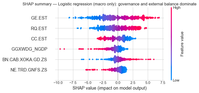

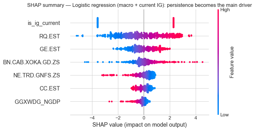
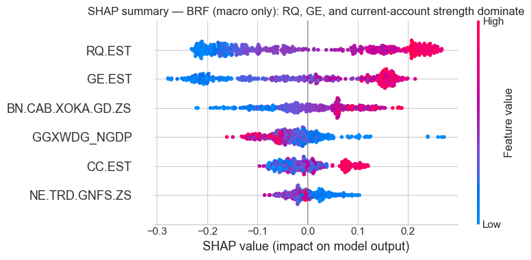
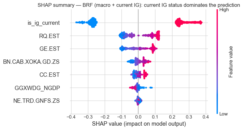
To complement the plots, the next block reports mean absolute SHAP importance.

# ------------------------------------------------------------
# Mean absolute SHAP importance tables
# ------------------------------------------------------------
shap_importance_logit = pd.DataFrame({
    "Feature": sov_features,
    "Mean |SHAP|": np.abs(logit_shap_vals.values).mean(axis=0)
}).sort_values("Mean |SHAP|", ascending=False)

shap_importance_logit_full = pd.DataFrame({
    "Feature": sov_features_v2,
    "Mean |SHAP|": np.abs(logit_full_shap_vals.values).mean(axis=0)
}).sort_values("Mean |SHAP|", ascending=False)

shap_importance_brf = pd.DataFrame({
    "Feature": sov_features,
    "Mean |SHAP|": np.abs(brf_macro_shap_exp.values).mean(axis=0)
}).sort_values("Mean |SHAP|", ascending=False)

shap_importance_brf_full = pd.DataFrame({
    "Feature": sov_features_v2,
    "Mean |SHAP|": np.abs(brf_full_shap_exp.values).mean(axis=0)
}).sort_values("Mean |SHAP|", ascending=False)

print("Mean absolute SHAP importance — Logistic (macro only):")
print(shap_importance_logit.round(4).to_string(index=False))

print("\nMean absolute SHAP importance — Logistic (macro + current IG):")
print(shap_importance_logit_full.round(4).to_string(index=False))

print("\nMean absolute SHAP importance — BRF (macro only):")
print(shap_importance_brf.round(4).to_string(index=False))

print("\nMean absolute SHAP importance — BRF (macro + current IG):")
print(shap_importance_brf_full.round(4).to_string(index=False))

Mean absolute SHAP importance — Logistic (macro only):
          Feature  Mean |SHAP|
           GE.EST       2.7084
           RQ.EST       1.9328
           CC.EST       1.3325
      GGXWDG_NGDP       0.9243
BN.CAB.XOKA.GD.ZS       0.8966
   NE.TRD.GNFS.ZS       0.8621

Mean absolute SHAP importance — Logistic (macro + current IG):
          Feature  Mean |SHAP|
    is_ig_current       2.9257
           RQ.EST       1.4836
           GE.EST       0.7859
BN.CAB.XOKA.GD.ZS       0.6734
   NE.TRD.GNFS.ZS       0.5222
           CC.EST       0.3759
      GGXWDG_NGDP       0.2559

Mean absolute SHAP importance — BRF (macro only):
          Feature  Mean |SHAP|
           RQ.EST       0.1589
           GE.EST       0.1287
BN.CAB.XOKA.GD.ZS       0.0618
      GGXWDG_NGDP       0.0459
           CC.EST       0.0431
   NE.TRD.GNFS.ZS       0.0265

Mean absolute SHAP importance — BRF (macro + current IG):
          Feature  Mean |SHAP|
    is_ig_current       0.2756
           RQ.EST       0.0846
           GE.EST       0.0666
BN.CAB.XOKA.GD.ZS       0.0253
           CC.EST       0.0189
      GGXWDG_NGDP       0.0127
   NE.TRD.GNFS.ZS       0.0058

These SHAP results are strikingly coherent across model classes.

In the macro-only logistic model, the dominant variables are the governance indicators, especially GE.EST and RQ.EST, followed by debt and current-account balance. So when the model must infer next-year IG status from fundamentals alone, it relies primarily on institutional quality, then on fiscal sustainability and external balance.

The macro-only BRF tells almost the same story, though with a different ordering: RQ.EST, GE.EST, and BN.CAB.XOKA.GD.ZS dominate. That is substantively important. It means that allowing non-linearity does not overturn the economic interpretation. The tree model is more flexible, but it is still relying on the same broad channels: institutions, external strength, and debt.

Once current IG status is added, the picture changes sharply. In both augmented models, is_ig_current becomes the dominant SHAP feature by a wide margin. That matches the earlier performance metrics exactly. Persistence is the strongest empirical regularity in the dataset, and the SHAP values make that visible directly rather than only through overall accuracy.

However, the fundamentals do not disappear. Even after controlling for current regime, the next most important variables remain RQ.EST, GE.EST, and current-account balance. So the augmented models are not saying that fundamentals are irrelevant. They are saying that fundamentals matter conditional on a very strong persistence anchor.

This is one of the clearest substantive conclusions in the whole modelling section. Across all four models, the economic story is stable:

without persistence, the models are driven mainly by governance, then by external balance and debt;
with persistence, current regime dominates, but governance remains the most important secondary signal.

Q2.4.12: Local SHAP Explanations: concrete sovereign narratives

Global SHAP tells us what matters on average. Local SHAP is more useful for understanding specific sovereign-year cases.

The benchmark cases below are chosen deliberately:

Azerbaijan 2023:actual upgrade missed by the persistence-aware models
Bahrain 2022: strong-looking non-IG case
Greece 2022: weak-looking IG-side candidate before re-entry to IG
Romania 2022: lower-end IG benchmark
Japan 2021: high-debt but clearly IG benchmark
Venezuela 2020 and Lebanon 2021: clear non-IG distress anchors

# ------------------------------------------------------------
# Local SHAP waterfall plots for benchmark sovereigns
# ------------------------------------------------------------
benchmark_cases = [
    ("Azerbaijan", 2023),
    ("Bahrain", 2022),
    ("Greece", 2022),
    ("Romania", 2022),
    ("Japan", 2021),
    ("Venezuela", 2020),
    ("Lebanon", 2021)
]

for country, year in benchmark_cases:
    idx_list = test_clean_v2.index[
        (test_clean_v2["country_clean"] == country) &
        (test_clean_v2["year"] == year)
    ].tolist()

    if not idx_list:
        continue

    idx = idx_list[0]
    row_pos = list(X_test_v2.index).index(idx)

    expl = shap.Explanation(
        values=brf_full_shap_exp.values[row_pos],
        base_values=brf_full_shap_exp.base_values[row_pos],
        data=X_test_v2.iloc[row_pos].values,
        feature_names=X_test_v2.columns.tolist()
    )

    plt.figure(figsize=(8, 5))
    shap.plots.waterfall(expl, max_display=10, show=False)
    plt.title(f"Local SHAP explanation — BRF (macro + current IG): {country}, {year}")
    plt.tight_layout()
    plt.show()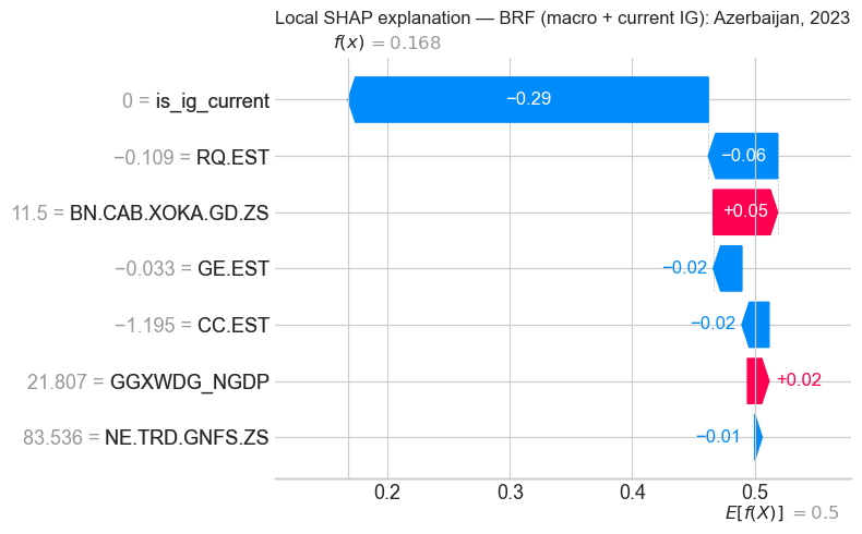

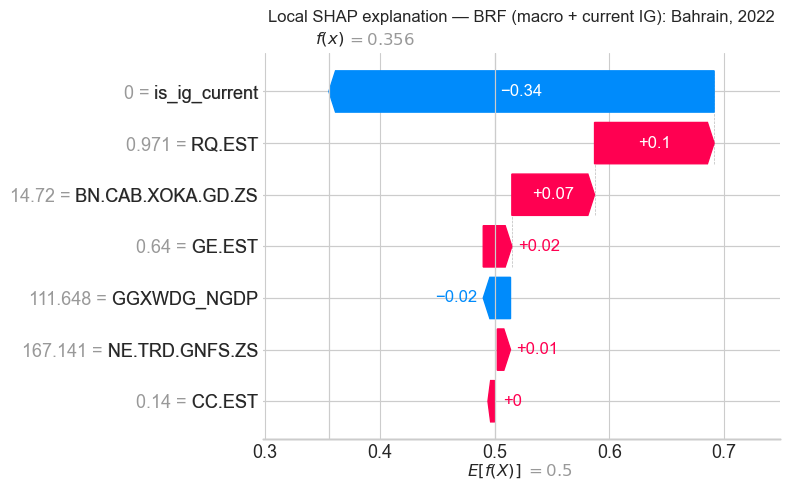
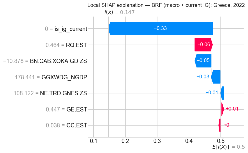
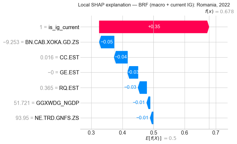
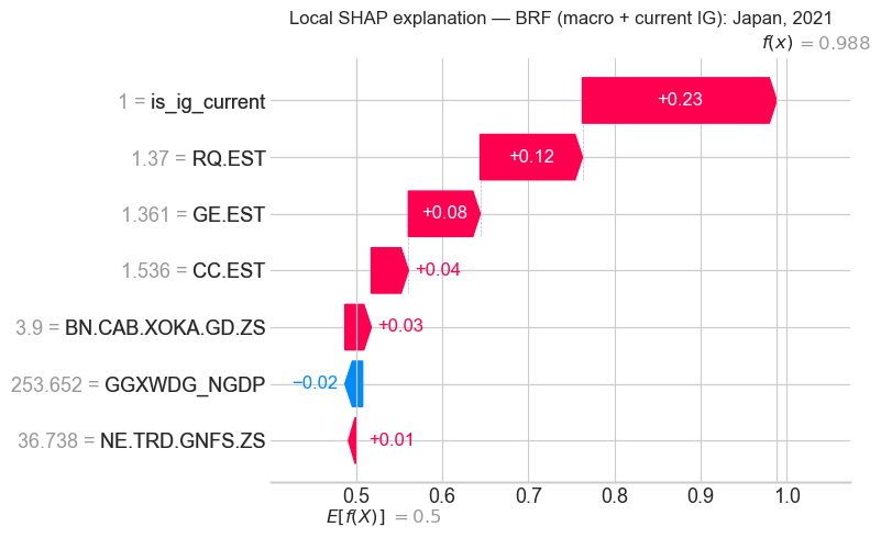
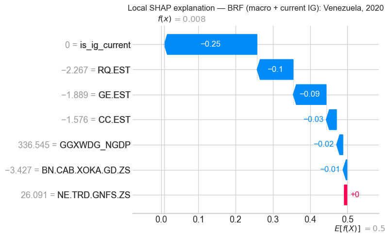
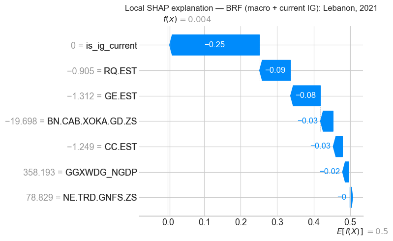
These local explanations are where the model becomes most interpretable in economic terms.

Azerbaijan 2023

Azerbaijan 2023 is especially informative because it is a genuine upgrade case that the persistence-aware models miss. The local SHAP plot shows that the largest negative contribution is simply current non-IG status, which pulls the probability down strongly. That drag is partly offset by a very strong current-account position and some support from governance, but not enough to push the persistence-aware prediction above the threshold.

This aligns closely with the earlier transition table. The macro-only logistic model gave Azerbaijan 2023 a probability of 0.9680, recognising that the sovereign’s fundamentals already looked strong enough to support IG re-entry. The persistence-aware models, however, remained anchored to the prior regime. So Azerbaijan is not a random miss. It is a case where external strength was strong enough to justify the upgrade on macro grounds, but not strong enough to overcome a model built to value persistence above all else.

Bahrain 2022

Bahrain 2022 is one of the clearest strong-looking non-IG cases. The local SHAP plot shows why. Even after the negative pull from current non-IG status, positive contributions from RQ.EST, current-account strength, and GE.EST lift the probability substantially. This matches the earlier feature-profile comparison almost perfectly: the strong-looking non-IG group was shown to have a much stronger external profile and much better governance than the median non-IG sovereign.

So Bahrain looks strong not because one variable is extreme in isolation, but because it combines better-than-usual institutions for a speculative sovereign with very strong external metrics.

Greece 2022

Greece 2022 is a useful weak-looking IG-side case. The local SHAP plot shows that the largest negative force is still current non-IG status, which is unsurprising because the country had not yet re-entered the IG regime at that point. But even beyond that, the plot shows sizeable negative pressure from current-account weakness and very high debt, with only modest positive contributions from governance.

That interpretation matches the broader evidence. In the profile comparison, weak-looking IG cases were characterised by very weak external balances and high debt burdens. Greece is a particularly clear example: although the institutional story had improved materially after the sovereign-debt crisis, the country still looked weak relative to the centre of the IG universe.

Romania 2022

Romania 2022 illustrates a different mechanism. Here, current IG status provides the main positive push. Most of the other features either contribute only modestly or pull the probability downward. This is exactly what the earlier “weak-looking IG” group comparison suggested: countries such as Romania remain IG, but their contemporaneous macro profile looks weak relative to stronger IG peers.

In that sense, the model is not denying Romania’s IG status. It is saying that Romania sits on the lower-quality edge of the IG group.

Japan 2021

Japan is not a borderline case, but it is a very useful benchmark. It combines very high public debt with an overwhelmingly strong IG probability. The local SHAP plot makes the reason explicit: the negative contribution from debt is more than offset by strong positive contributions from current IG status, RQ.EST, GE.EST, and CC.EST.

This is exactly the kind of case that shows why debt cannot be interpreted in isolation. Very high debt is not automatically incompatible with investment-grade status if it sits alongside exceptional institutional credibility, policy capacity, and domestic funding strength.

Venezuela 2020 and Lebanon 2021

These two cases are valuable for the opposite reason. They are not ambiguous at all. Their SHAP decompositions show that almost every major variable pushes in the same negative direction: current non-IG status, weak governance, weak external position, and very high debt vulnerability.

They serve as useful anchors. The real modelling difficulty is not distinguishing Japan from Venezuela or Lebanon. The real difficulty is separating the strong-looking speculative sovereigns from the weak-looking investment-grade sovereigns near the threshold.

Q2.4.13: What the supplementary analysis adds beyond the headline metrics

At this point, the post-model analysis has added several things that the raw metrics alone could not show.

First, the transition analysis shows that the persistence-aware models achieve extremely high average performance precisely because they fail to deviate from the current regime. They are excellent at reproducing no change, but they are unable to detect the rare threshold crossings that matter most economically.

Second, the within-tier analysis shows that the persistence-aware models also preserve the broad regime perfectly when the Fitch letter grade changes but the IG classification does not. The macro-only models are slightly less stable there, but that “instability” often reflects genuine tension between the macro profile and the official regime rather than random noise.

Third, the feature-profile comparison shows that the ambiguous sovereigns are not arbitrary curiosities. The weak-looking IG group and the strong-looking non-IG group occupy a genuinely mixed macro-institutional space between the two class centres.

Fourth, the grey-zone plot shows that these groups really do sit between the regimes in an interpretable feature space, rather than just near 0.5 in a black-box probability scale.

Fifth, the SHAP analysis identifies the variables doing the work. Across models, the same economic channels recur:

institutional quality
external balance
debt sustainability
and, when included, current IG status

So the disagreement between models is not really about the substantive economics. It is mainly about how much weight to place on persistence, and about how flexibly to model the remaining fundamentals.

Q2.4.14: Comparative synthesis of the models

Now that the metrics, transition results, profile comparisons, and SHAP evidence are all in place, the comparison can be made much more cleanly.

The next code blocks gather the main quantitative results in one place.

# ------------------------------------------------------------
# Overall model comparisons: train, CV, test
# ------------------------------------------------------------
comparison_all_train = pd.DataFrame({
    "Model": [
        "Persistence rule",
        "Logistic (macro only)",
        "Logistic (macro + current IG)",
        "BRF (macro only)",
        "BRF (macro + current IG)"
    ],
    "Balanced Accuracy": [
        balanced_accuracy_score(y_true_bench_train, y_pred_persist_train),
        balanced_accuracy_score(y_train, y_train_pred),
        balanced_accuracy_score(y_train_v2, y_train_pred_v2),
        balanced_accuracy_score(y_train, y_train_pred_rf_macro),
        balanced_accuracy_score(y_train_v2, y_train_pred_rf_full)
    ],
    "Macro F1": [
        f1_score(y_true_bench_train, y_pred_persist_train, average="macro"),
        f1_score(y_train, y_train_pred, average="macro"),
        f1_score(y_train_v2, y_train_pred_v2, average="macro"),
        f1_score(y_train, y_train_pred_rf_macro, average="macro"),
        f1_score(y_train_v2, y_train_pred_rf_full, average="macro")
    ],
    "ROC-AUC": [
        np.nan,
        roc_auc_score(y_train, y_train_prob),
        roc_auc_score(y_train_v2, y_train_prob_v2),
        roc_auc_score(y_train, y_train_prob_rf_macro),
        roc_auc_score(y_train_v2, y_train_prob_rf_full)
    ],
    "PR-AUC": [
        np.nan,
        average_precision_score(y_train, y_train_prob),
        average_precision_score(y_train_v2, y_train_prob_v2),
        average_precision_score(y_train, y_train_prob_rf_macro),
        average_precision_score(y_train_v2, y_train_prob_rf_full)
    ]
})

comparison_all_cv = pd.DataFrame({
    "Model": [
        "Persistence rule",
        "Logistic (macro only)",
        "Logistic (macro + current IG)",
        "BRF (macro only)",
        "BRF (macro + current IG)"
    ],
    "Balanced Accuracy": [
        np.nan,
        cv_logit_macro_summary["CV Balanced Accuracy"].iloc[0],
        cv_logit_full_summary["CV Balanced Accuracy"].iloc[0],
        cv_brf_macro_summary["CV Balanced Accuracy"].iloc[0],
        cv_brf_full_summary["CV Balanced Accuracy"].iloc[0]
    ],
    "Macro F1": [
        np.nan,
        cv_logit_macro_summary["CV Macro F1"].iloc[0],
        cv_logit_full_summary["CV Macro F1"].iloc[0],
        cv_brf_macro_summary["CV Macro F1"].iloc[0],
        cv_brf_full_summary["CV Macro F1"].iloc[0]
    ],
    "ROC-AUC": [
        np.nan,
        cv_logit_macro_summary["CV ROC-AUC"].iloc[0],
        cv_logit_full_summary["CV ROC-AUC"].iloc[0],
        cv_brf_macro_summary["CV ROC-AUC"].iloc[0],
        cv_brf_full_summary["CV ROC-AUC"].iloc[0]
    ],
    "PR-AUC": [
        np.nan,
        cv_logit_macro_summary["CV PR-AUC"].iloc[0],
        cv_logit_full_summary["CV PR-AUC"].iloc[0],
        cv_brf_macro_summary["CV PR-AUC"].iloc[0],
        cv_brf_full_summary["CV PR-AUC"].iloc[0]
    ]
})

comparison_all_test = pd.DataFrame({
    "Model": [
        "Persistence rule",
        "Logistic (macro only)",
        "Logistic (macro + current IG)",
        "BRF (macro only)",
        "BRF (macro + current IG)"
    ],
    "Balanced Accuracy": [
        balanced_accuracy_score(y_true_bench_test, y_pred_persist_test),
        balanced_accuracy_score(y_test, y_test_pred),
        balanced_accuracy_score(y_test_v2, y_test_pred_v2),
        balanced_accuracy_score(y_test, y_test_pred_rf_macro),
        balanced_accuracy_score(y_test_v2, y_test_pred_rf_full)
    ],
    "Macro F1": [
        f1_score(y_true_bench_test, y_pred_persist_test, average="macro"),
        f1_score(y_test, y_test_pred, average="macro"),
        f1_score(y_test_v2, y_test_pred_v2, average="macro"),
        f1_score(y_test, y_test_pred_rf_macro, average="macro"),
        f1_score(y_test_v2, y_test_pred_rf_full, average="macro")
    ],
    "ROC-AUC": [
        np.nan,
        roc_auc_score(y_test, y_test_prob),
        roc_auc_score(y_test_v2, y_test_prob_v2),
        roc_auc_score(y_test, y_test_prob_rf_macro),
        roc_auc_score(y_test_v2, y_test_prob_rf_full)
    ],
    "PR-AUC": [
        np.nan,
        average_precision_score(y_test, y_test_prob),
        average_precision_score(y_test_v2, y_test_prob_v2),
        average_precision_score(y_test, y_test_prob_rf_macro),
        average_precision_score(y_test_v2, y_test_prob_rf_full)
    ]
})

print("Training metrics:")
print(comparison_all_train.round(4).to_string(index=False))

print("\nCV metrics:")
print(comparison_all_cv.round(4).to_string(index=False))

print("\nTest metrics:")
print(comparison_all_test.round(4).to_string(index=False))

Training metrics:
                        Model  Balanced Accuracy  Macro F1  ROC-AUC  PR-AUC
             Persistence rule             0.9796    0.9803      NaN     NaN
        Logistic (macro only)             0.8894    0.8895   0.9604  0.9692
Logistic (macro + current IG)             0.9781    0.9789   0.9949  0.9956
             BRF (macro only)             0.9693    0.9678   0.9964  0.9974
     BRF (macro + current IG)             0.9781    0.9789   0.9985  0.9988

CV metrics:
                        Model  Balanced Accuracy  Macro F1  ROC-AUC  PR-AUC
             Persistence rule                NaN       NaN      NaN     NaN
        Logistic (macro only)             0.8474    0.8308   0.9455  0.9587
Logistic (macro + current IG)             0.9803    0.9799   0.9931  0.9941
             BRF (macro only)             0.8126    0.7883   0.9050  0.9387
     BRF (macro + current IG)             0.9710    0.9694   0.9908  0.9913

Test metrics:
                        Model  Balanced Accuracy  Macro F1  ROC-AUC  PR-AUC
             Persistence rule             0.9918    0.9918      NaN     NaN
        Logistic (macro only)             0.8681    0.8680   0.9425  0.9389
Logistic (macro + current IG)             0.9892    0.9892   0.9960  0.9966
             BRF (macro only)             0.8663    0.8663   0.9493  0.9487
     BRF (macro + current IG)             0.9910    0.9910   0.9978  0.9978

A visual comparison helps as well.

# ------------------------------------------------------------
# Visual comparison of train / CV / test metrics
# ------------------------------------------------------------
metrics = ["Balanced Accuracy", "Macro F1", "ROC-AUC", "PR-AUC"]

train_long = comparison_all_train[["Model"] + metrics].copy()
train_long["Sample"] = "Train"

cv_long = comparison_all_cv[["Model"] + metrics].copy()
cv_long["Sample"] = "CV mean"

test_long = comparison_all_test[["Model"] + metrics].copy()
test_long["Sample"] = "Test"

comparison_long = pd.concat([train_long, cv_long, test_long], ignore_index=True)

comparison_plot = comparison_long.melt(
    id_vars=["Model", "Sample"],
    value_vars=metrics,
    var_name="Metric",
    value_name="Value"
)

model_order = [
    "Persistence rule",
    "Logistic (macro only)",
    "Logistic (macro + current IG)",
    "BRF (macro only)",
    "BRF (macro + current IG)"
]

sample_order = ["Train", "CV mean", "Test"]

fig, axes = plt.subplots(4, 1, figsize=(10, 16))

for ax, metric in zip(axes, metrics):
    sub = comparison_plot[comparison_plot["Metric"] == metric].copy()
    sub["Model"] = pd.Categorical(sub["Model"], categories=model_order, ordered=True)
    sub["Sample"] = pd.Categorical(sub["Sample"], categories=sample_order, ordered=True)
    sub = sub.sort_values(["Model", "Sample"])

    sns.barplot(
        data=sub,
        x="Model",
        y="Value",
        hue="Sample",
        ax=ax,
        hue_order=sample_order
    )

    ax.set_title(metric, loc="left", fontweight="bold")
    ax.set_xlabel("")
    ax.set_ylabel("Score")
    ax.tick_params(axis="x", rotation=0)
    ax.grid(axis="y", linestyle="--", alpha=0.3)

    if ax.get_legend() is not None:
        ax.get_legend().remove()

handles, labels = axes[0].get_legend_handles_labels()
fig.legend(
    handles, labels,
    title="Sample",
    loc="center left",
    bbox_to_anchor=(1.02, 0.5),
    frameon=True
)

plt.tight_layout(rect=[0, 0, 0.95, 1])
plt.show()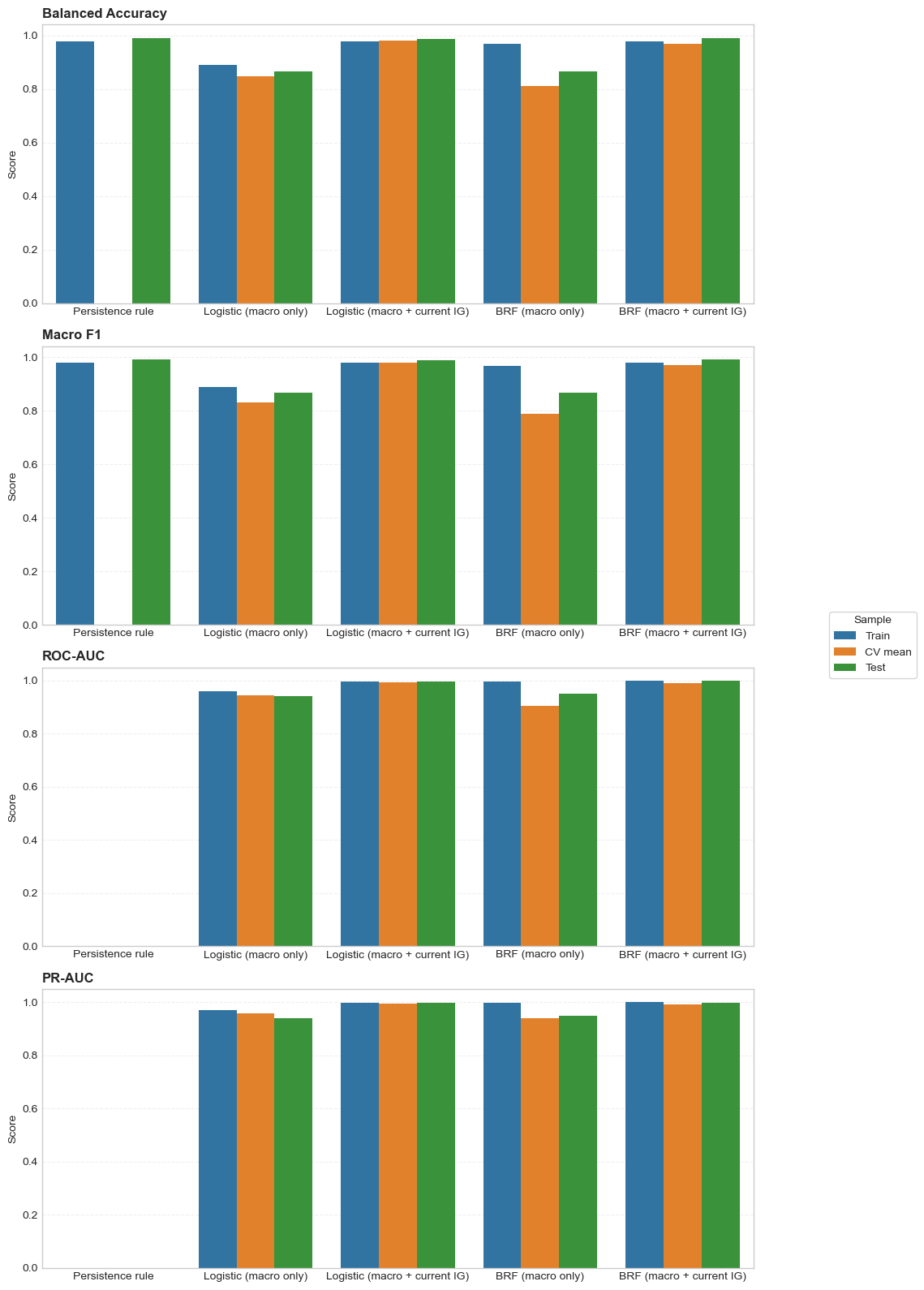

To make the generalisation pattern explicit, it is helpful to compute simple train–test and CV–test gaps.

# ------------------------------------------------------------
# Gap tables: train-test and CV-test
# ------------------------------------------------------------
gap_table = comparison_all_test.copy()
gap_table = gap_table.rename(columns={
    "Balanced Accuracy": "Test Balanced Accuracy",
    "Macro F1": "Test Macro F1",
    "ROC-AUC": "Test ROC-AUC",
    "PR-AUC": "Test PR-AUC"
})

gap_table["Train Balanced Accuracy"] = comparison_all_train["Balanced Accuracy"]
gap_table["Train Macro F1"] = comparison_all_train["Macro F1"]
gap_table["Train ROC-AUC"] = comparison_all_train["ROC-AUC"]
gap_table["Train PR-AUC"] = comparison_all_train["PR-AUC"]

gap_table["CV Balanced Accuracy"] = comparison_all_cv["Balanced Accuracy"]
gap_table["CV Macro F1"] = comparison_all_cv["Macro F1"]
gap_table["CV ROC-AUC"] = comparison_all_cv["ROC-AUC"]
gap_table["CV PR-AUC"] = comparison_all_cv["PR-AUC"]

gap_table["Train-Test Gap (BalAcc)"] = gap_table["Test Balanced Accuracy"] - gap_table["Train Balanced Accuracy"]
gap_table["Train-Test Gap (Macro F1)"] = gap_table["Test Macro F1"] - gap_table["Train Macro F1"]
gap_table["Train-Test Gap (ROC-AUC)"] = gap_table["Test ROC-AUC"] - gap_table["Train ROC-AUC"]
gap_table["Train-Test Gap (PR-AUC)"] = gap_table["Test PR-AUC"] - gap_table["Train PR-AUC"]

gap_table["CV-Test Gap (BalAcc)"] = gap_table["Test Balanced Accuracy"] - gap_table["CV Balanced Accuracy"]
gap_table["CV-Test Gap (Macro F1)"] = gap_table["Test Macro F1"] - gap_table["CV Macro F1"]
gap_table["CV-Test Gap (ROC-AUC)"] = gap_table["Test ROC-AUC"] - gap_table["CV ROC-AUC"]
gap_table["CV-Test Gap (PR-AUC)"] = gap_table["Test PR-AUC"] - gap_table["CV PR-AUC"]

print(gap_table.round(4).to_string(index=False))

Model  Test Balanced Accuracy  Test Macro F1  Test ROC-AUC  Test PR-AUC  Train Balanced Accuracy  Train Macro F1  Train ROC-AUC  Train PR-AUC  CV Balanced Accuracy  CV Macro F1  CV ROC-AUC  CV PR-AUC  Train-Test Gap (BalAcc)  Train-Test Gap (Macro F1)  Train-Test Gap (ROC-AUC)  Train-Test Gap (PR-AUC)  CV-Test Gap (BalAcc)  CV-Test Gap (Macro F1)  CV-Test Gap (ROC-AUC)  CV-Test Gap (PR-AUC)
             Persistence rule                  0.9918         0.9918           NaN          NaN                   0.9796          0.9803            NaN           NaN                   NaN          NaN         NaN        NaN                   0.0122                     0.0114                       NaN                      NaN                   NaN                     NaN                    NaN                   NaN
        Logistic (macro only)                  0.8681         0.8680        0.9425       0.9389                   0.8894          0.8895         0.9604        0.9692                0.8474       0.8308      0.9455     0.9587                  -0.0213                    -0.0214                   -0.0179                  -0.0303                0.0207                  0.0372                -0.0031               -0.0198
Logistic (macro + current IG)                  0.9892         0.9892        0.9960       0.9966                   0.9781          0.9789         0.9949        0.9956                0.9803       0.9799      0.9931     0.9941                   0.0111                     0.0103                    0.0011                   0.0009                0.0089                  0.0092                 0.0029                0.0025
             BRF (macro only)                  0.8663         0.8663        0.9493       0.9487                   0.9693          0.9678         0.9964        0.9974                0.8126       0.7883      0.9050     0.9387                  -0.1030                    -0.1015                   -0.0470                  -0.0487                0.0537                  0.0781                 0.0444                0.0100
     BRF (macro + current IG)                  0.9910         0.9910        0.9978       0.9978                   0.9781          0.9789         0.9985        0.9988                0.9710       0.9694      0.9908     0.9913                   0.0129                     0.0121                   -0.0007                  -0.0009                0.0200                  0.0216                 0.0071                0.0065

The comparison now supports a much more disciplined interpretation than a simple list of metric values.

1. Persistence is the dominant signal in the dataset

This is the central structural fact. The persistence benchmark achieves 0.9796 balanced accuracy in training and 0.9918 in testing. So any model given current regime has a very strong incentive to reproduce it.

That is exactly what the augmented models do. Their test metrics are extremely high:

Logistic (macro + current IG): balanced accuracy 0.9892, macro F1 0.9892, ROC-AUC 0.9960, PR-AUC 0.9966
BRF (macro + current IG): balanced accuracy 0.9910, macro F1 0.9910, ROC-AUC 0.9978, PR-AUC 0.9978

But the transition analysis showed the cost of that success: both augmented models get 0 of 5 test transitions right. So those excellent average metrics are achieved largely by reproducing the overwhelmingly common outcome of no change.

2. The macro-only models are weaker on average metrics, but more informative for actual regime change

The macro-only logistic regression achieves:

train balanced accuracy 0.8894, ROC-AUC 0.9604
CV mean balanced accuracy 0.8479, ROC-AUC 0.9454
test balanced accuracy 0.8681, ROC-AUC 0.9425

The macro-only BRF achieves:

train balanced accuracy 0.9693, ROC-AUC 0.9964
CV mean balanced accuracy 0.8126, ROC-AUC 0.9050
test balanced accuracy 0.8663, ROC-AUC 0.9493

So both macro-only models are clearly informative in a ranking sense, but neither comes close to persistence on threshold-based metrics. That is exactly what we would expect in a dataset where current regime already predicts next regime about 98.5% of the time.

However, the transition analysis showed that the macro-only models do something the persistence-aware models do not: they identify at least some actual upgrades and downgrades. The macro-only logistic gets 3 of 5 test transitions right; the macro-only BRF gets 2 of 5. That makes them more useful for signalling possible regime changes, even if their average classification metrics are lower.

3. BRF captures additional flexibility, but that flexibility is not equally stable across periods

In the macro-only setting, BRF fits the training data much more strongly than logistic regression. But the gap structure shows that this extra flexibility is not fully stable.

For the macro-only BRF:

train balanced accuracy = 0.9693
CV balanced accuracy = 0.8126
test balanced accuracy = 0.8663

and

train ROC-AUC = 0.9964
CV ROC-AUC = 0.9050
test ROC-AUC = 0.9493

So the BRF’s training performance is much stronger than the cross-validation evidence would justify. That is classic evidence of a flexible model fitting the training sample more tightly than its generalisation pattern supports.

Economically, that instability is plausible. The expanding-window folds do not represent identical environments. Earlier folds use shorter training windows and validate on smaller historical slices; later folds benefit from much longer training histories and include different macro-financial environments. The fact that the macro-only logistic model improves steadily across folds — balanced accuracy rising from 0.7212 in Fold 1 to 0.9272 in Fold 5 — suggests that a simpler linear mapping becomes more stable as more historical information accumulates. By contrast, the macro-only BRF is more erratic, with balanced accuracy ranging from 0.7349 to 0.9033 and ROC-AUC dipping as low as 0.8114 in one fold. That is exactly the kind of fold pattern one would expect when a flexible model is sensitive to regime-dependent interactions that are not equally stable across time.

4. Once persistence is included, model instability largely disappears

The augmented models look very different in cross-validation.

For logistic + current IG:

CV balanced accuracy 0.9803
CV ROC-AUC 0.9929
very small fold dispersion

For BRF + current IG:

CV balanced accuracy 0.9710
CV ROC-AUC 0.9908
again, very small fold dispersion

So once current regime is explicitly included, performance becomes both very high and much more stable across folds. This is not because the macro relationships suddenly become easier. It is because persistence overwhelms them. The current regime is so informative that differences in macro-financial environment matter much less for overall classification performance.

5. The economic story is stable across models even when the functional form changes

The SHAP results show that the models disagree less about the underlying economics than about the role of persistence.

Across the macro-only models, the same variables dominate:

GE.EST
RQ.EST
current-account balance
government debt

This is entirely consistent with the earlier EDA and with sovereign-credit intuition. The models are repeatedly telling the same substantive story: investment-grade status is shaped first by institutional quality, then by external strength, and then by fiscal sustainability.

So the move from logistic regression to BRF changes the functional form and the generalisation pattern, but not the broad economic narrative.

6. The real grey zone is between weak-looking IG and strong-looking non-IG sovereigns

This is where the profile comparison, grey-zone plot, and local SHAP analysis become essential.

The models are not confused by obvious extremes such as Japan on the clear IG side or Lebanon and Venezuela on the clear non-IG side. Those cases are economically coherent and model-consistent once interpreted in context.

The real ambiguity lies in sovereigns such as:

Greece, Romania, Mexico, Slovakia, Cyprus on the weak-looking IG side
Bahrain, Azerbaijan, Colombia, Panama on the strong-looking non-IG side

The profile comparison showed exactly why. The weak-looking IG group combines weaker governance, worse external balances, and higher debt than the median IG sovereign. The strong-looking non-IG group combines stronger governance and much stronger external metrics than the median non-IG sovereign.

That is a much more economically meaningful conclusion than simply saying that some sovereigns are “close to 0.5”. The models are identifying a substantive grey zone in the sovereign universe, not just producing noisy probabilities.

Q2.4.15: Conclusions so far

At this stage, the modelling results support four broad conclusions.

First, persistence dominates the binary prediction problem. That is why models with current IG status perform so well on average metrics and why the persistence benchmark is so hard to beat.

Second, macroeconomic and governance variables still contain meaningful information, especially for ranking sovereigns and identifying the grey zone closest to the IG threshold.

Third, the macro-only models reveal a stable and interpretable economic structure: institutions, current-account strength, and debt sustainability are the main channels associated with next-year IG status.

Fourth, the main difficulty of the exercise is not distinguishing obvious safe sovereigns from obvious distressed ones. It is distinguishing the relatively small set of strong-looking non-IG sovereigns from weak-looking IG sovereigns near the BBB− / BB+ boundary.

That is precisely where the binary rating problem is economically most consequential and where a macro-based model can still add value even when it cannot beat persistence on headline classification metrics.

2.5 Discussion

How predictable does sovereign IG status appear to be?

The first conclusion is that sovereign IG status is highly predictable in a mechanical sense, but much less predictable in the economically interesting sense.

At the broadest level, the binary target is extraordinarily persistent. The persistence benchmark achieves 0.9796 balanced accuracy in training and 0.9918 in testing, simply by predicting that next year’s IG status will be the same as the current year’s status. This is possible because only 22 out of 1,487 observations (1.5%) involve an actual crossing of the BBB− / BB+ threshold. So for the overwhelming majority of country-years, “no change” is the correct prediction.

That result immediately changes how predictability should be interpreted. If the question is merely “can we correctly predict next year’s IG label most of the time?”, the answer is yes, but largely because the target itself is so persistent. In that narrow sense, sovereign IG status appears highly predictable.

However, that is not the most economically meaningful question. The more important question is whether the model can identify the relatively small set of sovereigns that are at risk of crossing the threshold. On that harder task, predictability is much lower.

This is visible in the transition analysis. The persistence-aware models, i.e logistic regression with current IG status and BRF with current IG status, achieve extremely strong headline metrics, but they get 0 out of 17 training transitions and 0 out of 5 test transitions correct. They are excellent at reproducing the dominant outcome of no change, but essentially useless for identifying the rare regime changes that matter most for index inclusion, forced selling, and sovereign financing conditions.

By contrast, the macro-only models perform much worse on headline classification metrics, but they are the only ones that show meaningful sensitivity to actual threshold crossings. The macro-only logistic regression correctly identifies 11 of 17 training transitions and 3 of 5 test transitions; the macro-only BRF identifies 15 of 17 training transitions and 2 of 5 test transitions. So once the question is reframed from “can the model reproduce the dominant class?” to “can the model detect actual regime change?”, predictability becomes much more limited and much more uncertain.

The evidence therefore supports a nuanced conclusion: sovereign IG status is highly predictable as a persistent binary label, but much less predictable as a transition process. That distinction is central to the whole exercise.

Are macroeconomic variables alone sufficient to explain rating dynamics?

The answer is no, not fully.

The macroeconomic and institutional variables used here clearly contain meaningful information. Across the exploratory analysis, the macro-only logistic regression, the macro-only BRF, the profile comparisons, and the SHAP analysis, the same broad drivers recur:

institutional quality, especially government effectiveness and regulatory quality
external strength, especially the current-account balance
fiscal sustainability, especially government debt

So macroeconomic and governance indicators are clearly sufficient to explain an important part of the cross-sectional structure of sovereign credit risk. They help distinguish strong sovereigns from weak ones, and they help identify the “grey zone” between strong-looking non-IG and weak-looking IG sovereigns.

But they are not sufficient to explain all rating dynamics, especially near the threshold.

There are several reasons for this.

First, sovereign ratings are not based only on current or lagged macro outcomes. Rating agencies also incorporate more qualitative and forward-looking judgements about policy credibility, institutional reform, political stability, financing access, and the likely trajectory of risk rather than only its current level. Some of that is partially proxied by governance indicators, but much of it is not directly observed in the feature set used here.

Second, actual transitions are often triggered by discrete events that annual macro data cannot capture well. The clearest example is Russia 2021/2022: the downgrade is driven by geopolitical rupture and sanctions, not by gradual deterioration in lagged annual fundamentals. More generally, sovereign downgrades can be driven by sudden political crises, abrupt loss of market access, or event risk that is hard to anticipate from a small annual macro panel.

Third, the supplementary analysis showed that some sovereigns sit in mixed territory. Bahrain and Azerbaijan can look strong on external and governance dimensions while still remaining below IG. Romania, Greece, and Mexico can remain IG while looking weak relative to stronger IG peers. That means a model based only on macro and governance indicators may capture the broad structural logic of ratings, but still miss how agencies interpret borderline cases in practice.

So macro variables alone are informative, but not sufficient. They explain much of the long-run structure of sovereign creditworthiness, but not the full set of forces that drive actual rating actions.

What are the implications of treating panel observations as independent?

Treating the 1,487 country-year observations as if they were fully independent is a useful simplification for prediction, but it is not literally true, and that matters for interpretation.

The first issue is within-country temporal dependence. Sovereign ratings evolve slowly, and macro fundamentals also evolve gradually. So adjacent observations for the same country are highly correlated. A country rated IG in one year is very likely to remain close to that state in the next year unless a major shock occurs. This means the effective amount of information in the panel is smaller than the raw observation count suggests.

The second issue is cross-country dependence. Countries are jointly exposed to common global shocks, for example the COVID shock, the post-2021 inflation surge, tighter global financial conditions, or commodity-price shocks. So even observations from different countries are not fully independent when they occur in the same global environment.

These dependence structures have several implications.

First, they mean that the modelling results should be interpreted primarily as a predictive exercise, not as if each row were an independent experimental unit supporting strong causal claims.

Second, they mean that the apparent sample size can overstate the true amount of independent information. That is one reason why the persistence benchmark is so dominant and why it is dangerous to over-interpret headline performance metrics without the transition analysis and cross-validation evidence.

Third, they imply that coefficient interpretation in the logistic models must be handled cautiously. The coefficients are still useful descriptively — they tell us which variables are associated with higher or lower IG probability conditional on the others — but they should not be treated as if they came from a setting with independent observations and clean structural identification.

Finally, the panel structure also helps explain why time-aware validation was so important. A random split would have mixed closely related country-years across training and test sets and produced an over-optimistic assessment. The chronological split and expanding-window cross-validation are therefore not minor technical choices; they are essential to making the evaluation meaningful.

What are the main limitations of the modelling approach?

Several limitations are important.

First, the number of actual regime changes is very small. The panel contains 1,487 observations, but only 22 IG threshold crossings. That means the models are being asked to learn a rare event from relatively few examples. It also means that any conclusion about transition detection should be stated cautiously, because a difference of one or two correctly classified cases can materially change the apparent transition performance.

Second, the models rely on annual macroeconomic and governance data. That makes the framework transparent and manageable, but it also limits responsiveness. Annual data may miss short-run financial stress, sudden political deterioration, and market-based warning signals that appear much earlier than official macro releases.

Third, the binary target compresses a richer rating scale into a single threshold. That simplification is economically justified because the BBB− / BB+ boundary is institutionally important, but it also discards information. A movement from BBB to BBB− and a movement from AAA to AA+ are both treated as “still IG”, even though they may reflect different degrees of deterioration. Likewise, a sovereign just below the boundary and one deep in distress are both coded as non-IG.

Fourth, the feature set is incomplete. The selected predictors cover major channels of sovereign risk, but they do not include some potentially important determinants such as market-based funding conditions, debt maturity structure, reserve adequacy, contingent liabilities, electoral shocks, sanctions, or more direct measures of political instability.

Fifth, the panel structure complicates inference. As discussed above, country-years are not independent, and common shocks affect many observations at once. That does not invalidate the predictive exercise, but it does limit how strongly the results can be interpreted as evidence about stable structural parameters.

Sixth, the persistence-aware models illustrate a genuine modelling trade-off. Including current IG status produces excellent overall predictive performance, but it also causes the model to collapse toward persistence and lose sensitivity to actual threshold changes. So “better” headline metrics do not automatically mean a better model for every objective.

What extensions would be worth considering next?

Several extensions would be natural.

1. Model the full rating scale rather than only the binary IG/non-IG split. An ordinal model would preserve more information from the original Fitch scale and might distinguish better between sovereigns that are close to the threshold and those far from it.

2. Focus directly on transition risk rather than next-year class labels alone. A model designed explicitly for rare threshold crossings, or a survival / hazard framework modelling time until upgrade or downgrade, may be better aligned with the economically interesting part of the problem than a standard classifier.

3. Add market-based variables. Sovereign bond spreads, CDS spreads, exchange-rate stress, and financing-cost indicators are more forward-looking than annual macro variables and may improve detection of impending rating changes.

4. Add richer political and institutional information. The governance indicators used here are useful, but relatively broad. More specific measures of political instability, government turnover, conflict, sanctions exposure, or reform momentum could help explain cases where macro fundamentals alone are not enough.

5. Extend the time dimension. A longer historical panel would provide more threshold crossings and a richer range of crises, recoveries, and rating cycles. That would be especially valuable for learning the dynamics of rare transitions rather than only the persistence of the current regime.

6. Explore panel-specific methods. Approaches such as country fixed effects, random effects, hierarchical models, or clustered inference would better reflect the structure of the data, especially if the goal shifts from pure prediction toward more structural interpretation.

Overall conclusion

Taken together, the results suggest that sovereign IG status is easy to predict in the trivial sense that it is highly persistent, but much harder to predict in the economically meaningful sense of identifying actual regime changes.

Macroeconomic and governance variables are clearly informative. They capture a stable and interpretable structure centred on institutions, external strength, and debt sustainability, and they are useful for identifying the grey zone between weak-looking IG and strong-looking non-IG sovereigns.

But they are not sufficient on their own to explain all rating dynamics. Actual rating changes, especially threshold crossings, depend partly on event risk, political developments, market access, and qualitative agency judgement that are only imperfectly captured by the available predictors.

So the main contribution of the modelling exercise is not that it “solves” sovereign rating prediction. Rather, it shows that macro and institutional variables provide a meaningful and interpretable framework for organising sovereign credit risk, while also revealing the limits of a purely macro-based approach in a highly persistent panel setting.

References

Arena, Marco, Jaime Guajardo, Juan Yepez, Gerardo Peraza, Jorge Alvarez, Alain Brousseau, Emilio Fernandez Corugedo, and Hamid Faruqee. 2022. “Regional Spillovers from the Venezuelan Crisis.” Departmental Papers 2022 (019): 1. https://doi.org/10.5089/9798400224478.087.

Baur, Dirk G., Brian M. Lucey, and Thomas K. McDermott. 2010. “Is Gold a Safe Haven? International Evidence.” Journal of Banking and Finance 34 (8): 1886–98.

Cantor, Richard, and Frank Packer. 1996. “Determinants and Impact of Sovereign Credit Ratings.” Economic Policy Review 2 (2): 37–53.

Erb, Claude B., and Campbell R. Harvey. 2013. “The Golden Dilemma.” Financial Analysts Journal 69 (4): 10–42.

International Monetary Fund. Middle East and Central Asia Dept. 2023. “Lebanon.” IMF Staff Country Reports 2023 (237): 1. https://doi.org/10.5089/9798400247668.002.

Jaramillo, Laura, and Catalina Michelle Tejada. 2011. “Sovereign Credit Ratings and Spreads in Emerging Markets: Does Investment Grade Matter?” IMF Working Paper 11/44. Washington, DC: International Monetary Fund.

Saito, Ikuo. 2015. “Chapter 4. Japan’s Fiscal Risks.” In Can Abenomics Succeed?, ch004. USA: International Monetary Fund. https://doi.org/10.5089/9781498324687.071.ch004.

World Bank. 2023. “Lebanon Economic Monitor - Spring 2023 : The Normalization of Crisis Is No Road for Stabilization.” Text/{HTML}. World Bank. https://documents.worldbank.org/en/publication/documents-reports/documentdetail/099027005152320346.

Footnotes

The subsequent SHAP analysis also confirms these findings.↩︎