💻 Week 08 - Lab Roadmap (90 min)

DS202 - Data Science for Social Scientists

Author

Dr. Stuart Bramwell/Dr. Jon Cardoso-Silva

Published

14 November 2022

Context

This lab session draws on 🗓️ Week 04 lecture/workshop and 🗓️ Week 05 lecture content.

It also reuses elements of tidymodels introduced in previous labs where we used functions from library(broom) or library(rsample). These packages are part of tidymodels. For the record, tidymodel’s ‘Get Started’ tutorials are really good.

Important

Download this page as an RMarkdown file from Moodle.

Topics

More specifically, these are the things we will explore or revisit:

Difference between Classification vs Regression (🗓️ Week 03 lecture)
k-fold cross-validation
Support Vector Machine (SVM)
Hyperparameters

Setup

Setup

💡 Some of you have mentioned that your R version cannot handle tidymodels. We recommend you update R to version 4.2.0 or above.

Packages you will need

library('ISLR2')       # for the data
library('tidyverse')   # to use things like the pipe (%>%)
library('e1071')       # for SVM model
library('tidymodels')  # for model tuning, cross-validation etc.

# Vanity packages:
library('GGally')      # for pretty correlation plot
library('ggsci')       # for pretty plot colours
library('cvms')        # for pretty confusion matrix plots

The Data (10 min)

🍊Orange Juice

This week we will use a different ISLR2 dataset: OJ . We will perform a classification task with the goal to predict the Purchase column.

The data contains 1070 purchases where the customer either purchased Citrus Hill or Minute Maid Orange Juice. A number of characteristics of the customer and product are recorded.

ISLR2::OJ %>% head()

  Purchase WeekofPurchase StoreID PriceCH PriceMM DiscCH DiscMM SpecialCH
1       CH            237       1    1.75    1.99   0.00    0.0         0
2       CH            239       1    1.75    1.99   0.00    0.3         0
3       CH            245       1    1.86    2.09   0.17    0.0         0
4       MM            227       1    1.69    1.69   0.00    0.0         0
5       CH            228       7    1.69    1.69   0.00    0.0         0
6       CH            230       7    1.69    1.99   0.00    0.0         0
  SpecialMM  LoyalCH SalePriceMM SalePriceCH PriceDiff Store7 PctDiscMM
1         0 0.500000        1.99        1.75      0.24     No  0.000000
2         1 0.600000        1.69        1.75     -0.06     No  0.150754
3         0 0.680000        2.09        1.69      0.40     No  0.000000
4         0 0.400000        1.69        1.69      0.00     No  0.000000
5         0 0.956535        1.69        1.69      0.00    Yes  0.000000
6         1 0.965228        1.99        1.69      0.30    Yes  0.000000
  PctDiscCH ListPriceDiff STORE
1  0.000000          0.24     1
2  0.000000          0.24     1
3  0.091398          0.23     1
4  0.000000          0.00     1
5  0.000000          0.00     0
6  0.000000          0.30     0

To understand what each variable represent, open the R Console, type the following and hit ENTER:

?ISLR2::OJ

Which variables can help us distinguish the two different brands?

To simplify our plots later on, let’s focus on just two predictors:

plot_df <- ISLR2::OJ %>% select(Purchase, LoyalCH, PriceDiff)

g = (
  ggpairs(plot_df, aes(colour=Purchase))
  
  # Customizing the plot
  + scale_colour_startrek()
  + scale_fill_startrek()
  + theme_bw()
)
g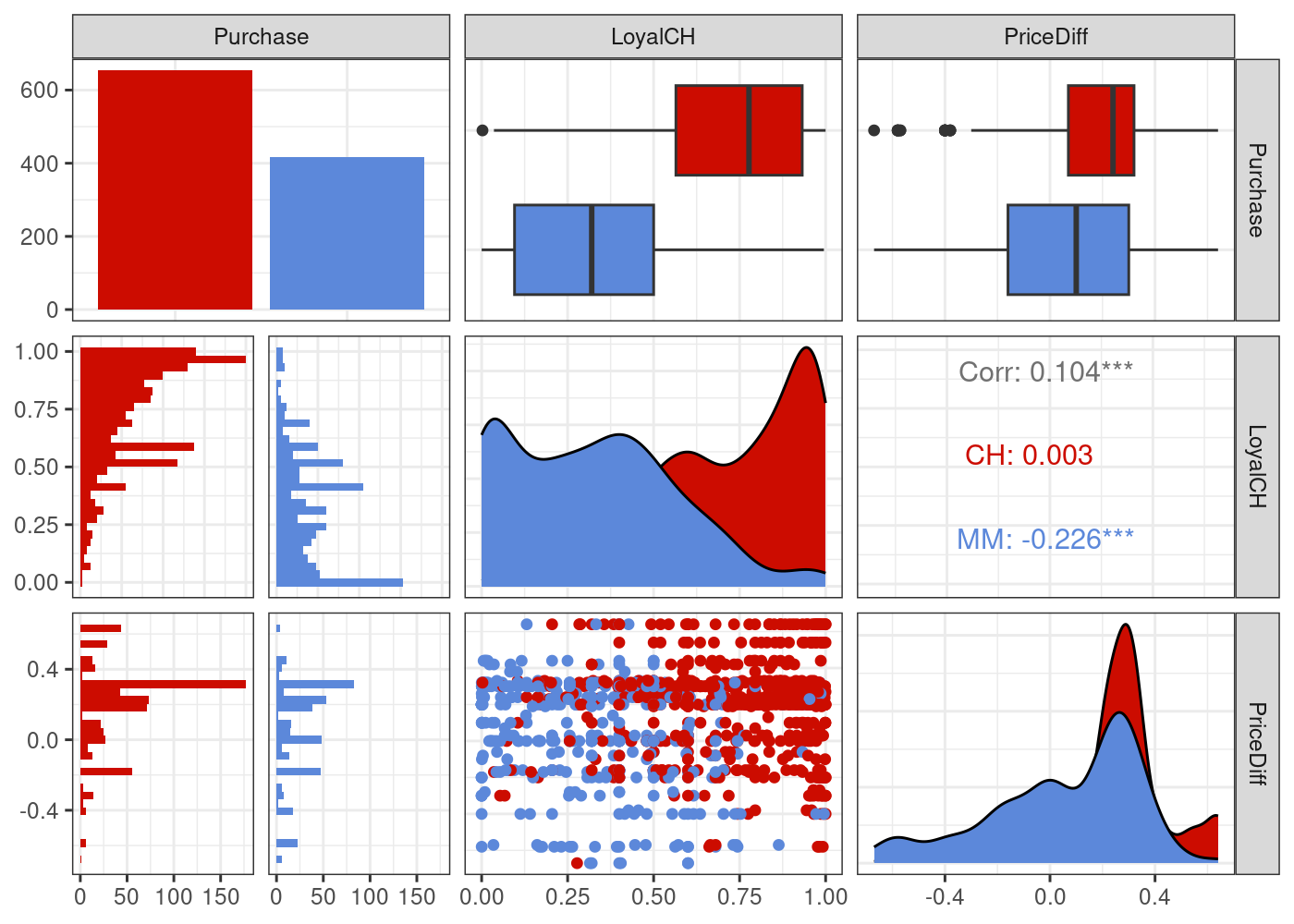

📈 Stock Market

We will also use the Smarket dataset from the ISLR2 package. We will perform a regression task with the goal to predict the percentage of return of the S&P 500 stock index on any given day, as represented by the Today column.

Daily percentage returns for the S&P 500 stock index between 2001 and 2005.

ISLR2::Smarket %>% head()

  Year   Lag1   Lag2   Lag3   Lag4   Lag5 Volume  Today Direction
1 2001  0.381 -0.192 -2.624 -1.055  5.010 1.1913  0.959        Up
2 2001  0.959  0.381 -0.192 -2.624 -1.055 1.2965  1.032        Up
3 2001  1.032  0.959  0.381 -0.192 -2.624 1.4112 -0.623      Down
4 2001 -0.623  1.032  0.959  0.381 -0.192 1.2760  0.614        Up
5 2001  0.614 -0.623  1.032  0.959  0.381 1.2057  0.213        Up
6 2001  0.213  0.614 -0.623  1.032  0.959 1.3491  1.392        Up

plot_df <- ISLR2::Smarket %>% select(Today, Volume, Lag1, Lag2)

g = (
  ggpairs(plot_df)
  
  # Customizing the plot
  + scale_colour_startrek()
  + scale_fill_startrek()
  + theme_bw()
)
g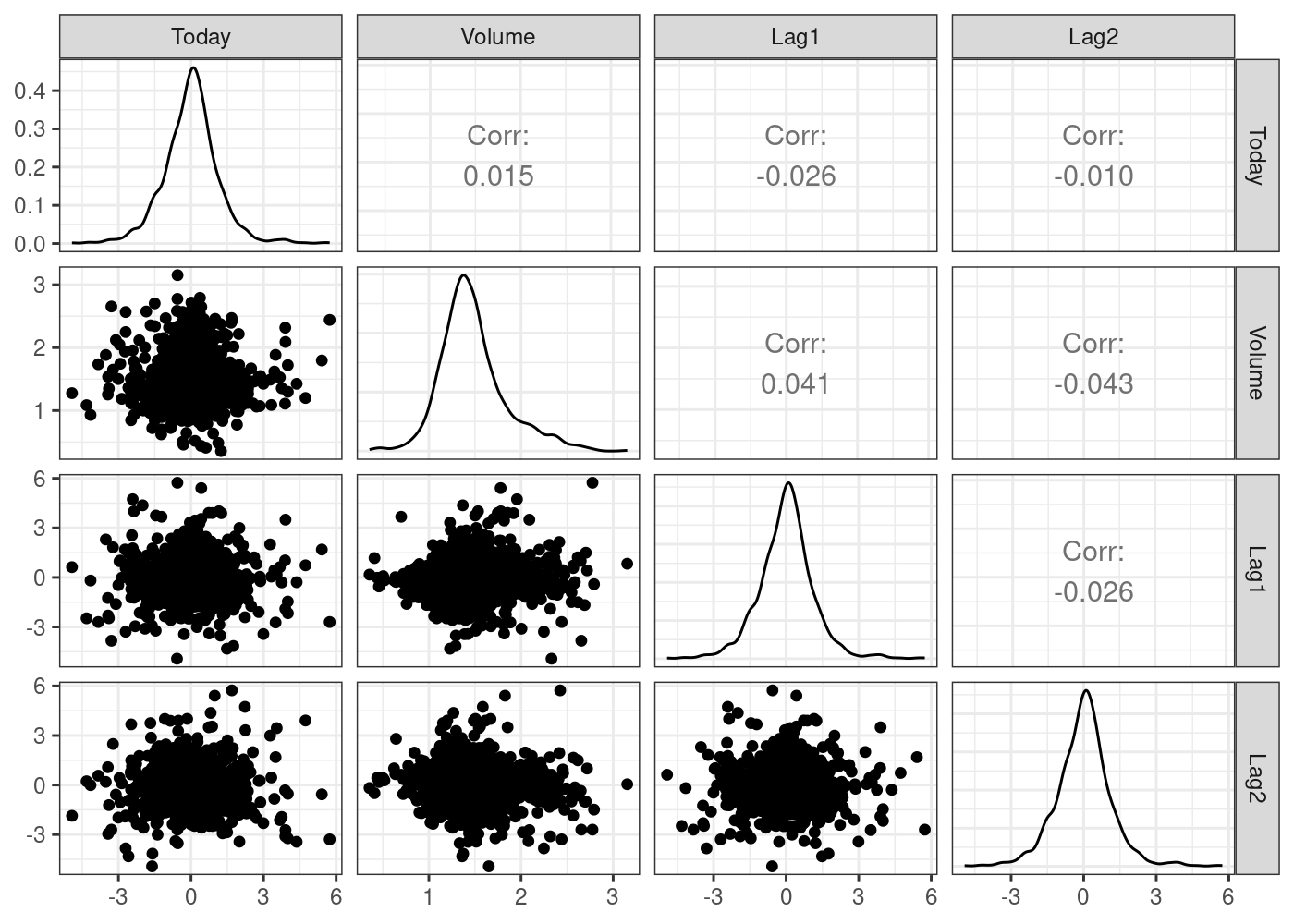

To understand what each variable represent, open the R Console, type the following and hit ENTER:

?ISLR2::Smarket

Step 1: SVM models for classification (30 min)

SVM stands for Support Vector Machines. Revisit 🗓️ Week 05 lecture or Chapter 9 of our textbook to understand more about this algorithm.

R does not come with SVM, so we need to import it from a library. Let’s start with the function svm we used in the Week 05 lecture, imported from the e1071 package. Here are a few things to know about the svm function:

The svm command is largely similar to other commands such as lm and glm in that the first parameter is an R formula and the second is the data set.
There are a few other options, but we will focus on specifying a radial kernel using kernel = 'radial'.
We can specify the type of machine learning task we are performing. Since we are doing classification, we use the option type = 'C-classification'.

Step 1.1: Train a SVM model

filtered_data <- ISLR2::OJ %>% select(Purchase, LoyalCH, PriceDiff)

orange_svm_model <- svm(Purchase ~ .,
                        data=filtered_data,
                        kernel='radial', 
                        type='C-classification')
orange_svm_model


Call:
svm(formula = Purchase ~ ., data = filtered_data, kernel = "radial", 
    type = "C-classification")


Parameters:
   SVM-Type:  C-classification 
 SVM-Kernel:  radial 
       cost:  1 

Number of Support Vectors:  427

🎯 ACTION POINT: What does the ‘Number of Support Vectors’ represent?

your text here

🎯 ACTION POINT: What would happened if we changed kernel to kernel="linear"?

your text here

Step 1.2: Goodness-of-Fit of the SVM

Let’s investigate how well our model fits the data. Let’s reuse the model we trained (orange_svm_model) and predict the same samples we used to train it. To avoid modifying our original dataframe, let’s save the output of the prediction in an auxiliary df (plot_df):

plot_df <- 
    filtered_data %>% 
    mutate(class_pred = predict(orange_svm_model, newdata = .))
head(plot_df)

Add a is_correct column to indicate whether the prediction was correct or not:

plot_df <- plot_df %>% mutate(is_correct = class_pred == Purchase)
head(plot_df)

  Purchase  LoyalCH PriceDiff class_pred is_correct
1       CH 0.500000      0.24         CH       TRUE
2       CH 0.600000     -0.06         CH       TRUE
3       CH 0.680000      0.40         CH       TRUE
4       MM 0.400000      0.00         MM       TRUE
5       CH 0.956535      0.00         CH       TRUE
6       CH 0.965228      0.30         CH       TRUE

Remember what we did in the Decision Tree example last week!

Simple confusion matrix:

confusion_matrix <- 
    table(expected=plot_df$Purchase, class_pred=plot_df$class_pred)
print(confusion_matrix)

Nicer looking confusion matrix:

plot_confusion_matrix(as_tibble(confusion_matrix), 
                      target_col = "expected", 
                      prediction_col = "class_pred",
                      
                      # Customizing the plot
                      add_normalized = TRUE,
                      add_col_percentages = FALSE,
                      add_row_percentages = FALSE,
                      counts_col = "n",
                      )

🎯 ACTION POINT: How well does the model fit the data? What is your opinion?

Measure: Precision

Remember from Week 04 Lecture/Workshop (notebook can be found under📥W04 Lecture Files on Moodle):

PRECISION: Given all predictions for a specific class, how many were True Positives? In other words, Precision = True Positives/(True Positives + False Positives).

Let’s calculate the score for the CH class. That is, as if CH=“Yes” and MM=“No”.

# expected == CH & predicted == CH
total_correct_CH   <- confusion_matrix["CH", "CH"]  

# sum of samples predicted == CH
total_predicted_CH <- sum(confusion_matrix[, "CH"]) 

precision          <- total_correct_CH/total_predicted_CH
cat(sprintf("%.2f%%", 100*precision))

85.27%

Measure: Recall

Also called True Positive Rate = True Positive/(True Positives + False Negatives)

# number of samples of brand CH
total_real_CH      <- sum(confusion_matrix["CH", ]) 

recall <- total_correct_CH/total_real_CH
cat(sprintf("%.2f%%", 100*recall))

87.75%

Measure: F1-SCORE

F1-SCORE: A combination of Precision and Recall

\[ \operatorname{F1-score} = \frac{2 \times \operatorname{Precision} \times \operatorname{Recall}}{(\operatorname{Precision} + \operatorname{Recall})} \]

f1_score <- (2*precision*recall)/(precision + recall)

cat(f1_score)

0.8649057

Step 1.3: Visualize the SVM decision space

Here we will demonstrate how you could simulate some data to cover the entire feature space of the data we are modelling. What do we mean by that? By inspecting LoyalCH and PriceDiff, we see the range values these variables can assume:

filtered_data %>% 
    select(c(LoyalCH, PriceDiff)) %>%
    summary()

    LoyalCH           PriceDiff      
 Min.   :0.000011   Min.   :-0.6700  
 1st Qu.:0.325257   1st Qu.: 0.0000  
 Median :0.600000   Median : 0.2300  
 Mean   :0.565782   Mean   : 0.1465  
 3rd Qu.:0.850873   3rd Qu.: 0.3200  
 Max.   :0.999947   Max.   : 0.6400

💡 We can simulate data to account for all possible combinations of LoyalCH and PriceDiff. We achieve this using crossing, another tidyverse function:

We feed crossing a sequence of numbers that range from the minimal and maximal values of both variables, incremented by 0.1 values.
We then create a new variable class_pred which uses the SVM model object to predict the brand of orange juice purchased by the customer
Note that we say newdata = . to indicate that we simply want to use the data set created with crossing as our new data.

sim.data <- 
  crossing(LoyalCH   = seq(0,1,0.05),
           PriceDiff = seq(-1,1,0.1)) %>% 
  mutate(class_pred = predict(orange_svm_model, newdata = .))
head(sim.data)

# A tibble: 6 × 3
  LoyalCH PriceDiff class_pred
    <dbl>     <dbl> <fct>     
1       0      -1   MM        
2       0      -0.9 MM        
3       0      -0.8 MM        
4       0      -0.7 MM        
5       0      -0.6 MM        
6       0      -0.5 MM

The data above is all synthetic (“fake”)! But it is very useful to colour the background of our plot.

We use geom_tile to show the area the SVM model identifies as Chinstrap penguins. We then use geom_point to overlay the actual data. Red dots in blue areas and vice versa indicate cases where the SVM model makes errors.

g <- (
  plot_df %>%   
    ggplot()
  
    # Tile the background of the plot with SVM predictions
    + geom_tile(data = sim.data, aes(x=LoyalCH, y=PriceDiff, fill = class_pred), alpha = 0.25)
  
    # Actual data
    + geom_point(aes(x=LoyalCH, y=PriceDiff, colour = Purchase, shape = is_correct), size=2.5, stroke=0.95, alpha=0.7)
  
    # Define X and Os
    + scale_shape_manual(values = c(4, 1))
    
    # (OPTIONAL) Customizing the colours and theme of the plot
    + scale_x_continuous(labels=scales::percent)
    + scale_colour_startrek()
    + scale_fill_startrek()
    + theme_minimal()
    + theme(panel.grid = element_blank(), legend.position = 'bottom', plot.title = element_text(hjust = 0.5))
    + labs(x = 'Customer brand loyalty for CH', y = 'Sale price of MM less sale price of CH', fill = 'Brand', colour = 'Brand', shape = 'Correct prediction?', title = sprintf('Overall Training Accuracy = %.2f %%', 100*(sum(plot_df$correct)/nrow(plot_df))))
)

g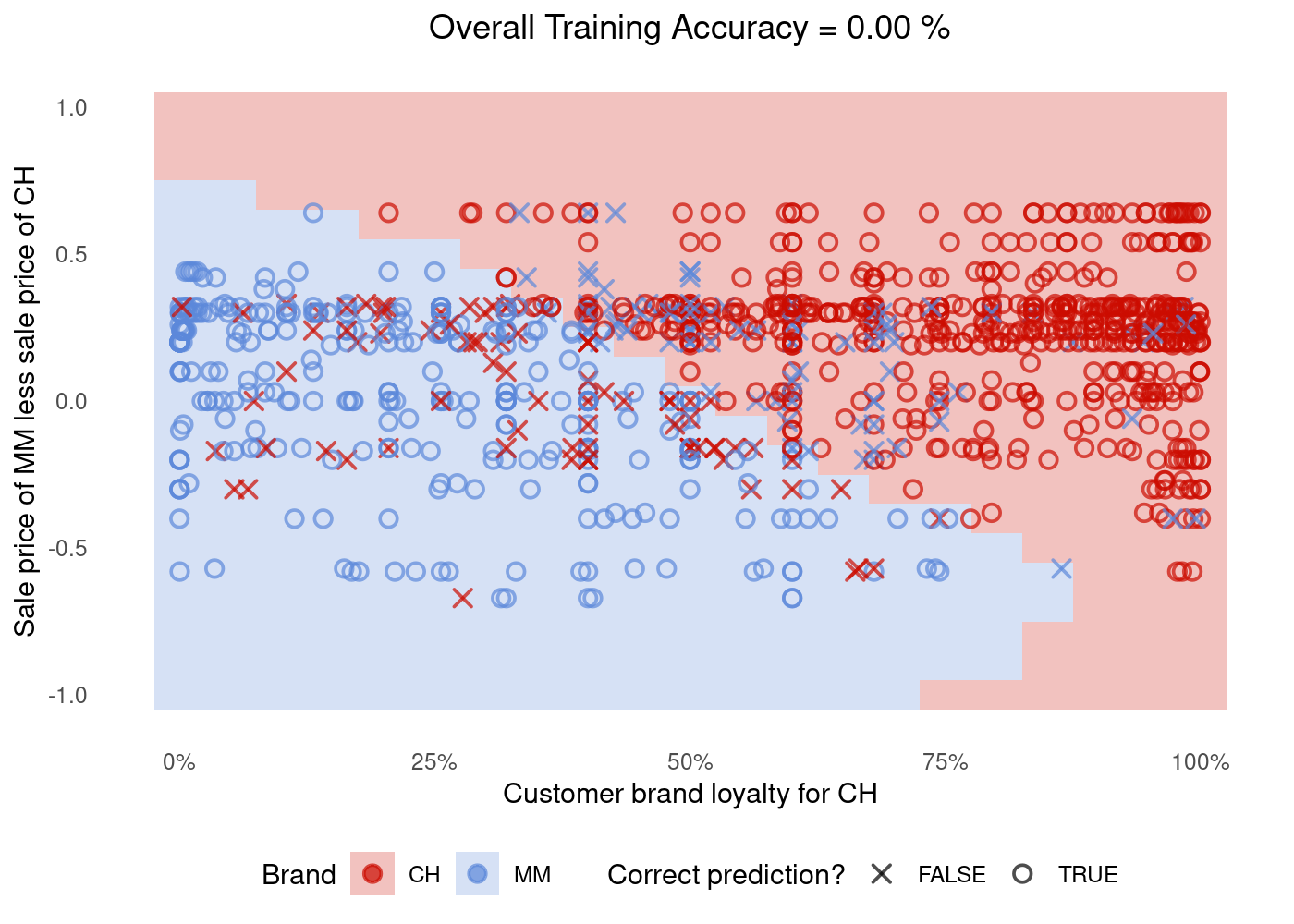

🤝 WORKING TOGETHER In pairs, discuss what you see in the plot:

What do the shape of dots represent? The X and Os?

your text here

What do the colours of the dots represent?

your text here

What do the background colour in the plot represent?

your text here

Can you point in the plot roughly which dots you would expect to be the support vectors?

Step 2: Doing the same with tidymodels (20 min)

Step 2: Doing the same with `tidymodels` (20 min)

The function svm from library(e1071) package is not the only way to run SVM in R. The package parsnip also have its own SVM functions. The functionality is roughly the same but there are differences in how you write the code.

parsnip already comes installed in tidymodels, so we do not need to import or install anything else.

Step 2.1 Training the SVM model

We specify a radial basis function SVM (see the part about kernels in the 🗓️ Week 05 lecture) with the function svm_rbf.

In the spirit of tidyverse, we pipe the SVM algorithm into the fit function, where we can define the R formula like we have been doing with other algorithms:

orange_tidymodel <-
  svm_rbf() %>% 
  set_mode('classification') %>% 
  fit(Purchase ~ ., data = filtered_data)

orange_tidymodel

parsnip model object

Support Vector Machine object of class "ksvm" 

SV type: C-svc  (classification) 
 parameter : cost C = 1 

Gaussian Radial Basis kernel function. 
 Hyperparameter : sigma =  1.65374574360967 

Number of Support Vectors : 432 

Objective Function Value : -386.8495 
Training error : 0.170093 
Probability model included.

🎯 ACTION POINT: Compare the output above to that of another colleague. Why don’t you get the exact same output?

your personal notes go here

💡 If you want to try different kernels, you will need to replace svm_rbf() by svm_linear() or svm_poly().

Step 2.2: Goodness-of-Fit of the SVM

Let’s investigate how well our model fits the data. Let’s reuse the model we trained (orange_tidymodel) and predict the same samples we used to train it.

Function augment(<model>, <df>) of tidymodels applies a model to a dataframe and return the same data plus a few columns:

plot_df <- augment(orange_tidymodel, filtered_data)
head(plot_df)

🎯 ACTION POINT: How is the plot_df data frame above different to the first plot_df we created in Step 1.2?

your notes go here

Add a is_correct column to indicate whether the prediction was correct or not:

plot_df <- plot_df %>% mutate(is_correct = .pred_class == Purchase)
head(plot_df)

# A tibble: 6 × 7
  Purchase LoyalCH PriceDiff .pred_class .pred_CH .pred_MM is_correct
  <fct>      <dbl>     <dbl> <fct>          <dbl>    <dbl> <lgl>     
1 CH         0.5        0.24 CH             0.862    0.138 TRUE      
2 CH         0.6       -0.06 CH             0.718    0.282 TRUE      
3 CH         0.68       0.4  CH             0.876    0.124 TRUE      
4 MM         0.4        0    MM             0.174    0.826 TRUE      
5 CH         0.957      0    CH             0.879    0.121 TRUE      
6 CH         0.965      0.3  CH             0.876    0.124 TRUE

Measure: Precision

You don’t need to calculate precision by hand, just use the precision() function from tidymodels:

plot_df %>% precision(Purchase, .pred_class) %>% head()

# A tibble: 1 × 3
  .metric   .estimator .estimate
  <chr>     <chr>          <dbl>
1 precision binary         0.856

Measure: Recall

You don’t need to calculate recall by hand, just use the recall() function from tidymodels:

plot_df %>% recall(Purchase, .pred_class) %>% head()

# A tibble: 1 × 3
  .metric .estimator .estimate
  <chr>   <chr>          <dbl>
1 recall  binary         0.867

Measure: F1-score

You don’t need to calculate F1-score by hand, just use the f_meas() function from tidymodels:

plot_df %>% f_meas(Purchase, .pred_class) %>% head()

# A tibble: 1 × 3
  .metric .estimator .estimate
  <chr>   <chr>          <dbl>
1 f_meas  binary         0.861

(Optional) ROC curve

Plot the ROC curve for class Purchase=="CH" :

plot_df %>% 
  roc_curve(Purchase, .pred_CH) %>% 
  autoplot

Warning: Returning more (or less) than 1 row per `summarise()` group was deprecated in
dplyr 1.1.0.
ℹ Please use `reframe()` instead.
ℹ When switching from `summarise()` to `reframe()`, remember that `reframe()`
  always returns an ungrouped data frame and adjust accordingly.
ℹ The deprecated feature was likely used in the yardstick package.
  Please report the issue at <https://github.com/tidymodels/yardstick/issues>.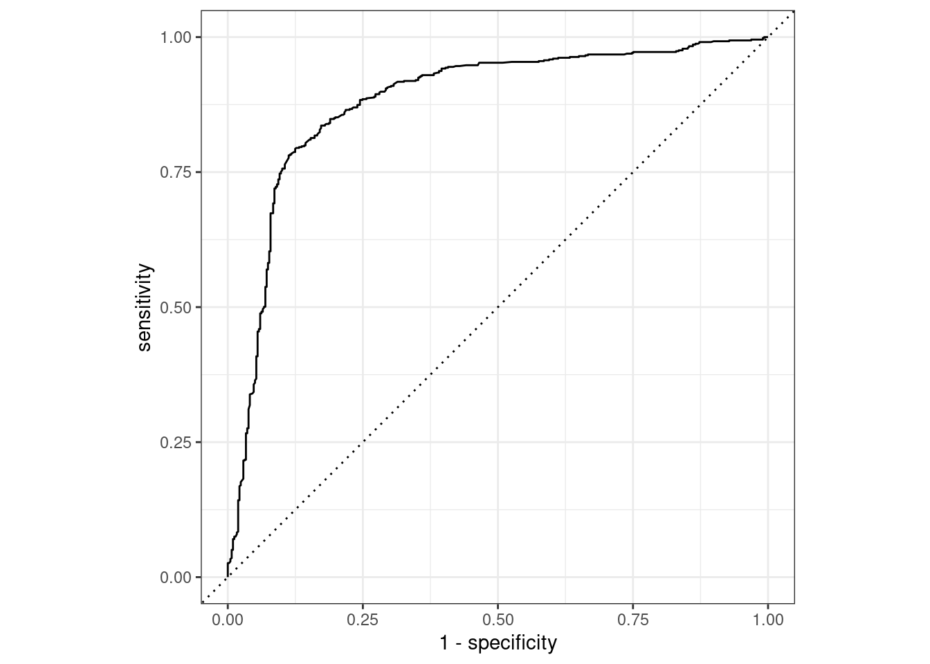

🏠 Take-home exercise Q1:

Edit the cell below modifying event_level from "second" to "first". Why do you get different results? What do you think is going on?

plot_df %>% f_meas(Purchase, .pred_class, event_level=...)

💡Tip: Read the documentation of f_meas to understand what event_level represents. (Type ?f_meas)

💡 Gold Tip: note the Levels of the factor variable called Purchase:

plot_df$Purchase

🏠 Take-home exercise Q2:

Create a plot of the confusion matrix for the orange_tidymodel like we did in Step 1.

## your code goes here

🏠 Take-home exercise Q3:

Create a plot of SVM decision space for the orange_tidymodel like we did in Step 1.

## your code goes here

🎯 ACTION POINT: If you were to run the SVM algorithm by yourself in another dataset, which version would you prefer, the one in Step 1 or the one in Step 2?

your notes go here

Step 3: What about regression? (30 min)

Here we will be using the 📈 SMarket data.

Step 3.1: Train the model

Let’s select just the predictors Volume and Lag1 and fit a regression model to predict Today:

# Remove Direction, otherwise we would be "cheating" 
filtered_data <- ISLR2::Smarket %>% select(Today, Volume, Lag1)

smarket_tidymodel <-
  svm_rbf() %>% 
  set_mode('regression') %>% 
  fit(Today ~ ., data = filtered_data)

smarket_tidymodel

parsnip model object

Support Vector Machine object of class "ksvm" 

SV type: eps-svr  (regression) 
 parameter : epsilon = 0.1  cost C = 1 

Gaussian Radial Basis kernel function. 
 Hyperparameter : sigma =  1.79706099888903 

Number of Support Vectors : 1117 

Objective Function Value : -760.8719 
Training error : 0.927028

Step 3.2: Goodness-of-Fit of the SVM

Since the target variable is continuous, not discrete, we cannot plot confusion matrix nor anything like that. We will have to go back to the idea of residuals (🗓️ Week 02 Lecture & 💻 Week 03 - Lab).

plot_df <- 
  augment(smarket_tidymodel, filtered_data) %>% 
  mutate(row_number=row_number()) # adding this here just to make our plot easier
plot_df %>% head()

# A tibble: 6 × 6
   Today Volume   Lag1   .pred .resid row_number
   <dbl>  <dbl>  <dbl>   <dbl>  <dbl>      <int>
1  0.959   1.19  0.381 -0.0565  1.02           1
2  1.03    1.30  0.959 -0.256   1.29           2
3 -0.623   1.41  1.03  -0.263  -0.360          3
4  0.614   1.28 -0.623  0.261   0.353          4
5  0.213   1.21  0.614 -0.153   0.366          5
6  1.39    1.35  0.213 -0.149   1.54           6

🎯 ACTION POINT: What do the different columns mean?

your text go here

Now, let’s look at the distribution of residuals and let’s mark the absolute residuals above 2 to flag the worst predictions (2 was an arbitrary choice, it all depends on the context):

g <- (
  ggplot(plot_df, aes(x=row_number, y=.resid))
  + geom_point(alpha=0.6)
  
  + theme_bw()
  + geom_hline(yintercept = c(-2,2), color="red", linetype="dashed")
  + labs(title="Distribution of residuals (the closer to zero the better)")
)

g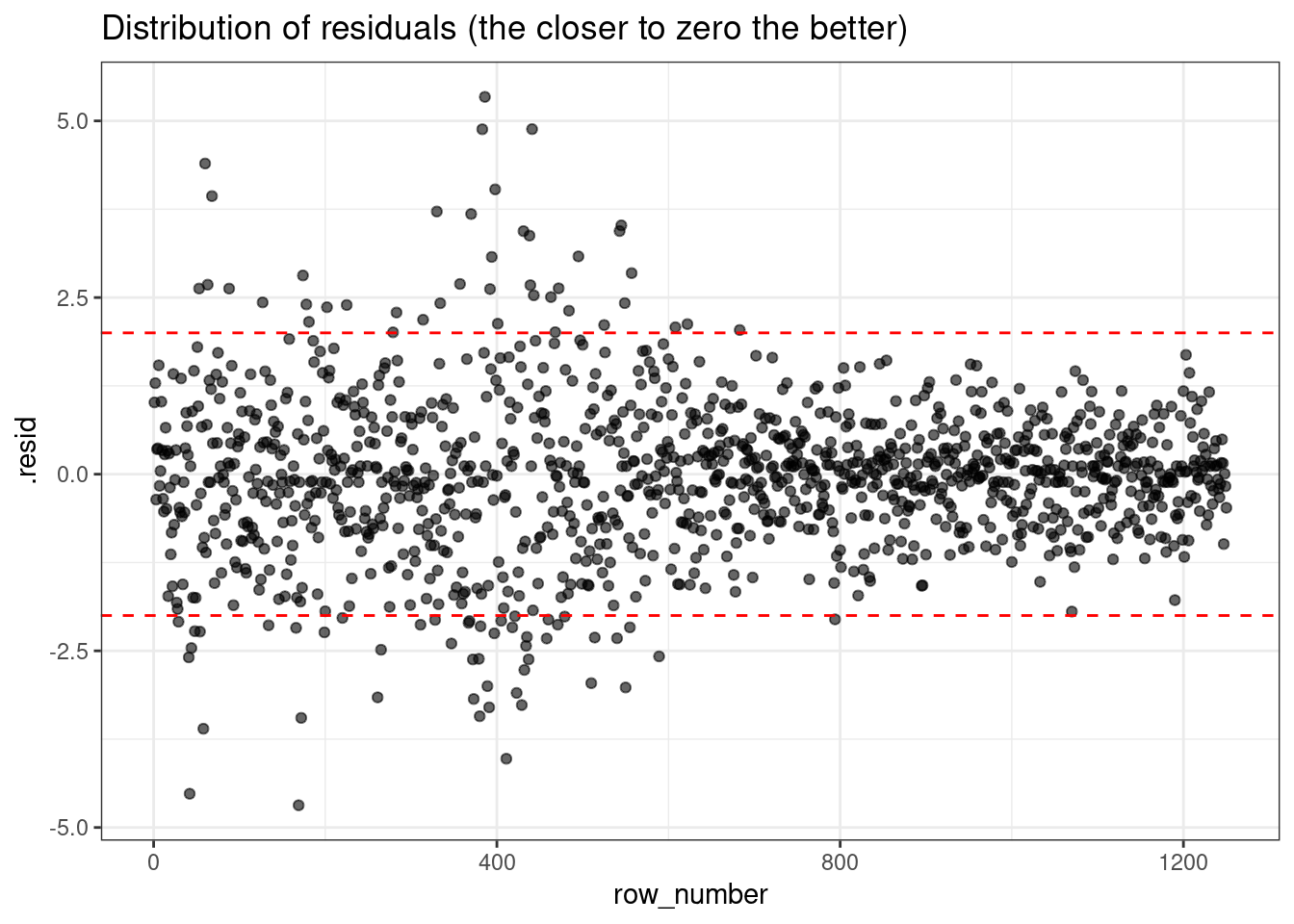

Measure: Mean Absolute Error (MAE)

\[ MAE = \frac{\sum_{i=1}^{n}{|y_i - \hat{y}_i|}}{n} \]

plot_df %>% mae(Today, .pred)

# A tibble: 1 × 3
  .metric .estimator .estimate
  <chr>   <chr>          <dbl>
1 mae     standard       0.789

Measure: Root Mean Squared Error (RMSE)

\[ RMSE = \frac{\sum_{i=1}^{n}{(y_i - \hat{y}_i)^2}}{n} \]

plot_df %>% rmse(Today, .pred)

# A tibble: 1 × 3
  .metric .estimator .estimate
  <chr>   <chr>          <dbl>
1 rmse    standard        1.09

🎯 ACTION POINT: Would a better model have a larger or smaller value of MAE/RMSE?

your text goes here

Step 3.3 Visualize the SVM decision space (Regression)

Now, let’s replicate what we did in Step 1.3 only this time for the Smarket data and using predictions from the smarket_tidymodel.

We start by summarising the data. We want to find out the minimum and maximal values that the columns Volumn and Lag1 reach:

filtered_data %>% 
    select(c(Volume, Lag1)) %>%
    summary()

     Volume            Lag1          
 Min.   :0.3561   Min.   :-4.922000  
 1st Qu.:1.2574   1st Qu.:-0.639500  
 Median :1.4229   Median : 0.039000  
 Mean   :1.4783   Mean   : 0.003834  
 3rd Qu.:1.6417   3rd Qu.: 0.596750  
 Max.   :3.1525   Max.   : 5.733000

Then, we create a simulated dataset with combinations of the Volume and Lag1 columns:

sim.data <- 
  crossing(Volume   = seq(0,3.5,0.1),
           Lag1 = seq(-5,6,0.2))
sim.data <- augment(smarket_tidymodel, sim.data)
head(sim.data)

# A tibble: 6 × 3
  Volume  Lag1   .pred
   <dbl> <dbl>   <dbl>
1      0  -5   -0.0103
2      0  -4.8 -0.0103
3      0  -4.6 -0.0103
4      0  -4.4 -0.0103
5      0  -4.2 -0.0103
6      0  -4   -0.0103

💡 Look at the entire dataset with View(sim.data)

Looking back at the plot of residuals, let’s flag the worst predictions, those with an absolute residual above 2.

plot_df$residual_above_2 <- (plot_df$.resid) > 2

g <- (
  plot_df %>%   
    ggplot()
  
    ## Tile the background of the plot with SVM predictions
    + geom_tile(data = sim.data, aes(x=Volume, y=Lag1, fill = .pred), alpha = 0.45)
  
    ## Actual data
    + geom_point(aes(x=Volume, y=Lag1, colour = residual_above_2, shape = residual_above_2, alpha=residual_above_2), size=2.5, stroke=0.95)
  
    ## Define X and Os
    + scale_shape_manual(values = c(4, 1))
    + scale_fill_viridis_c()
    + scale_color_manual(values=c("black", "red"))
    + scale_alpha_manual(values=c(0.1, 0.7))
    
    ## (OPTIONAL) Customizing the colours and theme of the plot
    + theme_minimal()
    + theme(panel.grid = element_blank(), legend.position = 'bottom', plot.title = element_text(hjust = 0.5))
    + labs(x = 'Volume', y = 'Lag 1', fill = "Today's Prediction", colour = 'Residual above 2?', shape = 'Residual above 2?', alpha='Residual above 2?', title='Worst predictions are marked as red circles')
)

g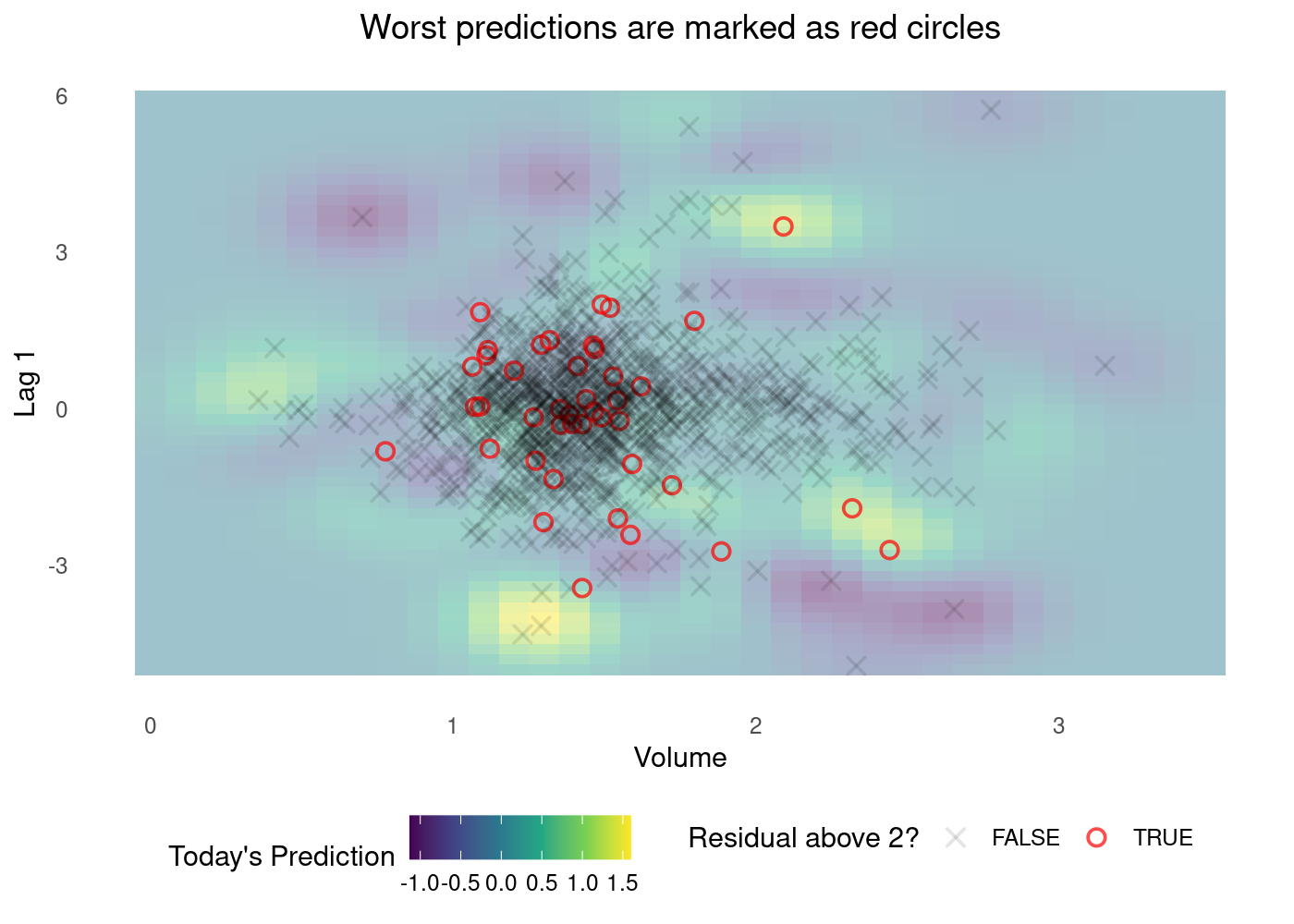

💡 The plot above might not be as easy to understand as the one for classification.

Step 3.3: Understand the parameters of `svm_rbf`

The svm_rbf function has three parameters you can tune:

cost
rbf_sigma
margin

🎯 ACTION POINT: Train your abilities to interact with code documentation. Type ?svm_rbf and hit ENTER. What do these parameters represent?

💡 Tip: At the bottom of the help page, you will find a link to kernlab engine details that has more useful info about SVM RBF.

your text goes here

Step 3.4: Tweak the parameters

🤝 WORKING TOGETHER In pairs, change the values of cost, rbf_sigma and margin in the chunk below and run the other two chunks of code to look at the distribution of residuals and summary metrics.

Discuss your findings. Can you find any combination of values that makes the model better? Or any that makes it worse?

alternative_smarket_model <-
  svm_rbf(cost=1, rbf_sigma=10, margin=0.9) %>% 
  set_mode('regression') %>% 
  fit(Today ~ ., data = filtered_data)

alternative_smarket_model

parsnip model object

Support Vector Machine object of class "ksvm" 

SV type: eps-svr  (regression) 
 parameter : epsilon = 0.9  cost C = 1 

Gaussian Radial Basis kernel function. 
 Hyperparameter : sigma =  10 

Number of Support Vectors : 401 

Objective Function Value : -195.7568 
Training error : 0.832623

Residuals plot

plot_df <- 
  augment(alternative_smarket_model, filtered_data) %>% 
  mutate(row_number=row_number()) ## adding this here just to make our plot easier

g <- (
  ggplot(plot_df, aes(x=row_number, y=.resid))
  + geom_point(alpha=0.6)
  
  + theme_bw()
  + geom_hline(yintercept = c(-2,2), color="red")
)

g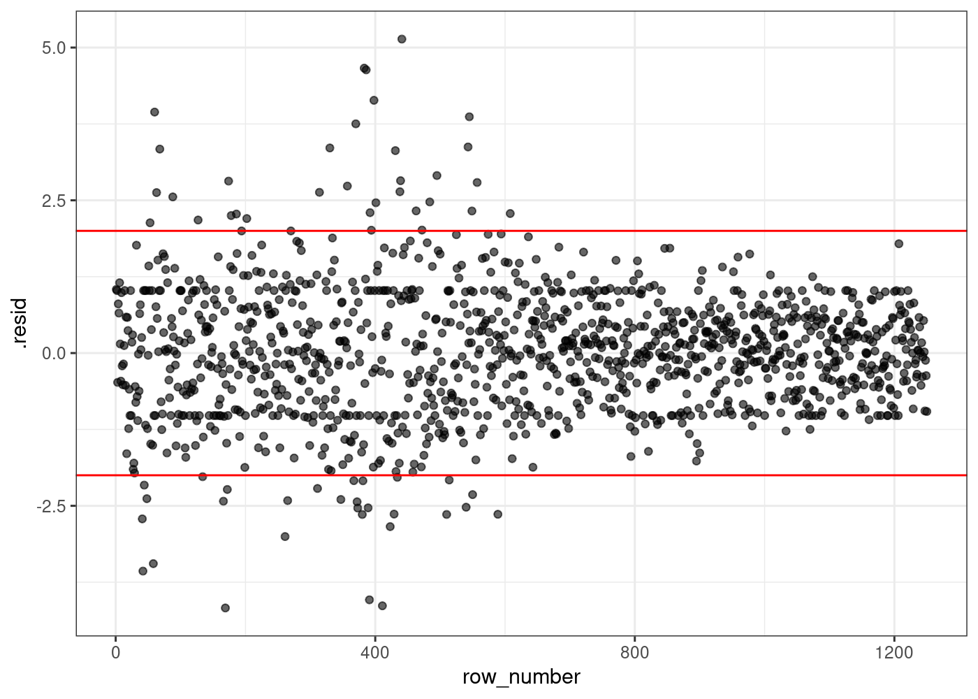

Metrics

## Use the vectorized version of MAE and RMSE functions
plot_df %>% summarise(mae=mae_vec(Today, .pred),
                      rmse=rmse_vec(Today, .pred))

# A tibble: 1 × 2
    mae  rmse
  <dbl> <dbl>
1 0.787  1.04

🏠 Take-home exercise Q4:

Retrain the model in Step 3 for Smarket, this time using svm_linear instead of svm_rbf.
Reuse the code in Step 3.4 to replicate the plots and metric calculations for this new model.
Which model fits the target variable (Today) better?

# your code goes here

your text goes here

Want to take it to the next level? (Optional)

Want to take it to the next level? (Optional)

In a separate, more advanced, bonus lab roadmap we show how to perform k-fold cross-validation using tidymodels to tune the parameters of SVM automatically.

It is optional, you don’t need to read it, but it might be the best way to solidify your knowledge of SVM and its parameters.

Setup

The Data (10 min)

🍊Orange Juice

📈 Stock Market

Step 1: SVM models for classification (30 min)

Step 1.1: Train a SVM model

Step 1.2: Goodness-of-Fit of the SVM

Simple confusion matrix:

Nicer looking confusion matrix:

Measure: Precision

Measure: Recall

Measure: F1-SCORE

Step 1.3: Visualize the SVM decision space

Step 2: Doing the same with tidymodels (20 min)

Step 2.1 Training the SVM model

Step 2.2: Goodness-of-Fit of the SVM

Measure: Precision

Measure: Recall

Measure: F1-score

(Optional) ROC curve

🏠 Take-home exercise Q1:

🏠 Take-home exercise Q2:

🏠 Take-home exercise Q3:

Step 3: What about regression? (30 min)

Step 3.1: Train the model

Step 3.2: Goodness-of-Fit of the SVM

Measure: Mean Absolute Error (MAE)

Measure: Root Mean Squared Error (RMSE)

Step 3.3 Visualize the SVM decision space (Regression)

Step 3.3: Understand the parameters of svm_rbf

Step 3.4: Tweak the parameters

🏠 Take-home exercise Q4:

Want to take it to the next level? (Optional)

Step 2: Doing the same with `tidymodels` (20 min)

Step 3.3: Understand the parameters of `svm_rbf`