Identifying outliers in linear model

DS202 Blog Post

TLDR

Here you will find R code to single out points with high “studentized” residuals

During Week 03 lab, we looked at diagnostic plots we can generate in R to obtain insights about the fit of a linear model.

Import required libraries

library(ISLR2)
library(tidyverse)

Fit a linear model then produce diagnostic plots

lm.fit <- lm(medv ~ lstat * age , data = ISLR2::Boston)

par(mfrow=c(2,2))
plot(lm.fit)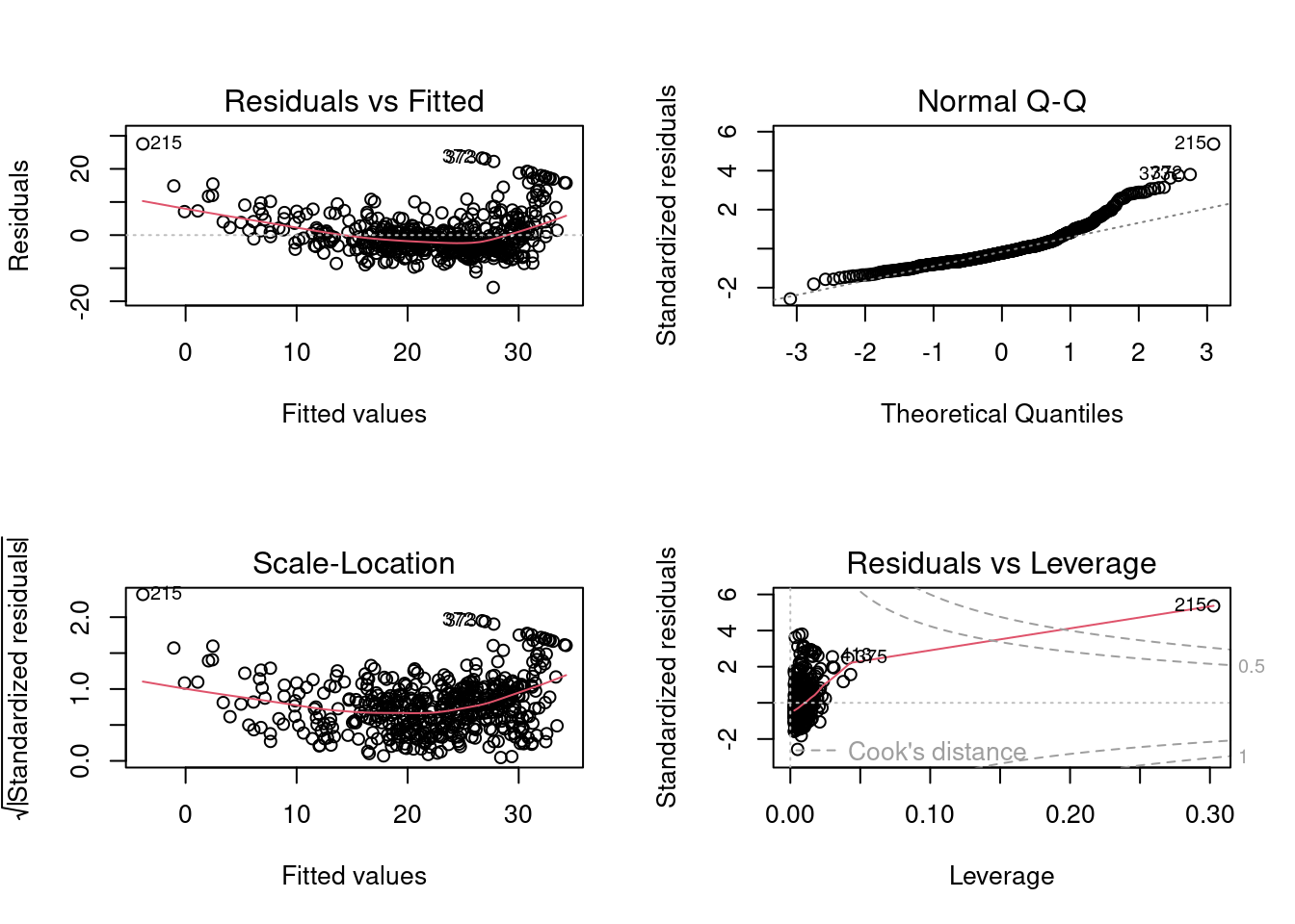

A frequent question we got in the labs was about the first of these plots, “Residuals vs Fitted”.

Residual vs Fitted plot

Ideally, the residual plot, also called the null residual plot, should show a random scatter of points centered around 0 and forming an approximately constant width band.

base R

Code

# Add dots
plot(predict(lm.fit), rstudent(lm.fit), 
     xlab="Fitted values",
     ylab="Residuals",
     main="Residuals vs Fitted")

# Add lines
abline(h = 3, lwd = 5,col = 'red')
abline(h = 0, lwd = 5,col = 'yellow')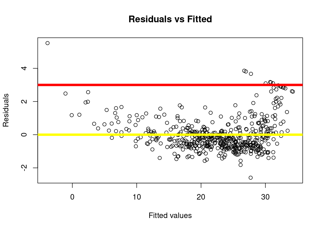

tidyverse

Code

plot_df <- data.frame(fitted_vals=predict(lm.fit),
                      residuals=rstudent(lm.fit))

g <- ggplot(plot_df, aes(x=fitted_vals, y=residuals)) +

    # Add dots
     geom_point(alpha=0.4, size=3.5) +
     xlab("Fitted values") +
     ylab("Residuals") +
     ggtitle("Residuals vs Fitted") +

    # Add lines
    geom_hline(yintercept=0, size=1.5, color='yellow') +
    geom_hline(yintercept=3, size=1.5, color='red') +

    # Customising the plot +
     theme_bw()

Warning: Using `size` aesthetic for lines was deprecated in ggplot2 3.4.0.
ℹ Please use `linewidth` instead.

Code

g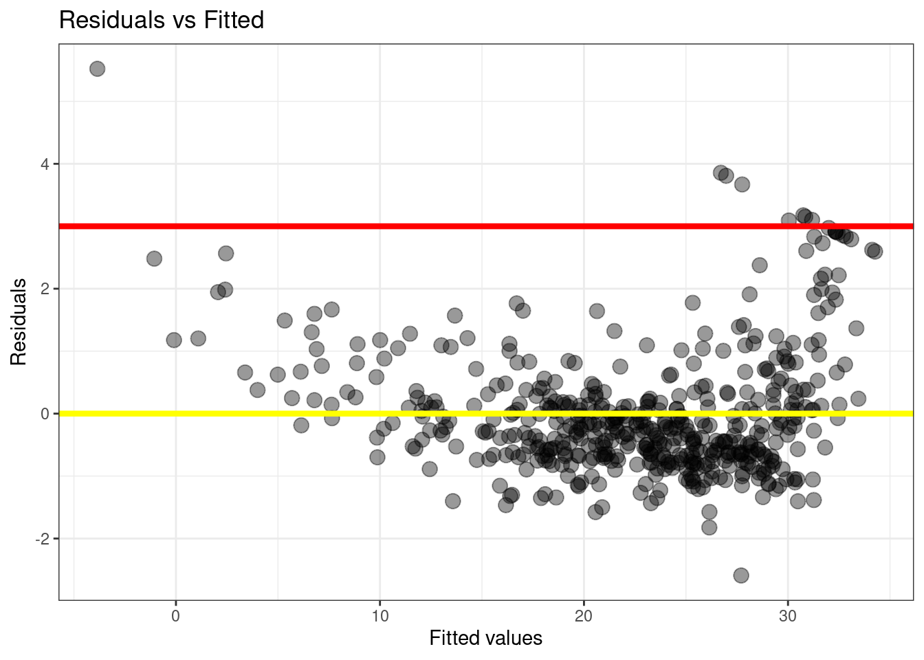

Selecting outliers

How do you identify the data points that have a high value of residuals (potential outliers)?

To produce this plot, we used the function rstudent() to calculate the so-called “studentized” residuals. This function returns a vector with the same length as the number of data points:

studentized_residuals <- rstudent(lm.fit)
length(studentized_residuals)

[1] 506

nrow(Boston)

[1] 506

We can use this information to filter and select those data points that produced a studentized-residual above 3:

df_potential_outliers <- Boston[studentized_residuals > 3, ]
df_potential_outliers

       crim zn indus chas   nox    rm   age    dis rad tax ptratio lstat medv
187 0.05602  0  2.46    0 0.488 7.831  53.6 3.1992   3 193    17.8  4.45 50.0
215 0.28955  0 10.59    0 0.489 5.412   9.8 3.5875   4 277    18.6 29.55 23.7
226 0.52693  0  6.20    0 0.504 8.725  83.0 2.8944   8 307    17.4  4.63 50.0
258 0.61154 20  3.97    0 0.647 8.704  86.9 1.8010   5 264    13.0  5.12 50.0
263 0.52014 20  3.97    0 0.647 8.398  91.5 2.2885   5 264    13.0  5.91 48.8
268 0.57834 20  3.97    0 0.575 8.297  67.0 2.4216   5 264    13.0  7.44 50.0
372 9.23230  0 18.10    0 0.631 6.216 100.0 1.1691  24 666    20.2  9.53 50.0
373 8.26725  0 18.10    1 0.668 5.875  89.6 1.1296  24 666    20.2  8.88 50.0

Data frame df_potential_outliers above contain all potential outliers according to this criteria. In a real-life setting, you would check the values of these data points in comparison with the rest of the dataset to understand what makes them different.

What to do next?

If the process that generated the dataset is indeed linear, it is possible that these are “true” outliers, rare cases that deviate from the norm. But often, this indicates that a linear model is not able to capture all the nuances present in the data. Maybe the data generating procedure is nonlinear? Or maybe it depends on other features that are not present in your dataset?

As for your next actions, it all depends on what you plan to do with this model or how much risk you can take by predicting data similar to these edge cases. If you do not want or cannot afford to ignore these errors, you can try to collect more data, fit more complex algorithms, or talk to domain experts to try to understand these cases a bit more.