✔️ Summative Problem Set 03 | Solutions

DS202 - Data Science for Social Scientists

Author

Dr. Jon Cardoso-Silva

Here you will find model solutions to the third Summative Problem Set of DS202 (2022/23).

🥇 It is not uncommon that we are more pleased with solutions provided by the students than the template ones we created. The answers on this page were compiled and adapted from a student submission and shared here with their permission.

Q1. Linear Regression (5 points)

Click to remember the question

> What metric does Ordinary Least Square (OLS) optimise? And how does OLS estimate regression coefficients?

OLS minimises the sum of the squared residuals. Thus, it optimises mean squared error (MSE) and root mean squared error (RMSE). RMSE is often used over MSE because it is standardised to the same unit as the outcome variable, facilitating interpretation.

Assuming this is a simple regression predicting the outcome variable y from the predictor x:

the OLS method first calculates the mean of y and the mean of x
then, for every data point, it deducts the corresponding mean from every true value of x and y (e.g., y - mean of y), which results in the error of every data point
then, for every data point, it multiplies the error for y and the corresponding error of x and subsequently sums the result of the multiplications, which is the absolute error: \[ A = \sum{ [(y_i - \bar{y}) \times (x_i - \bar{x})]} \]
then, it calculates the error for x (the residual), squares these values, and calculates the sum of these squared residuals \[ B = \sum{ [(x_i - \bar{x})^2]} \]
with that information, it can calculate the slope estimate B1 by dividing A by B, or it can combine steps 3 and 4 into one formula (see full formula below) \[ \beta_1 = \frac{A}{B} \] \[ \beta_1 = \frac{\sum{ [(y_i - \bar{y}) \times (x_i - \bar{x})]}}{\sum{ [(x_i - \bar{x})^2]}} \]
After having a value for \(\beta_1\) and the means of y and x, it can calculate the intercept coefficient \(\beta_0\) with the following formula: \[ \beta_0 = \bar{y} - \beta_1 \times \bar{x} \]

And this is how OLS estimates coefficients.

These formulas aim to find the coefficients \(\beta_0\) and \(\beta_1\) that minimise the residual sum of squares (the sum of the squared error of all data points, RSS). The same logic (minimising the RSS) is applied when estimating coefficients for multiple regression, but the math becomes more complicated and necessitates statistical software.

📑 What we liked about this response

Although points 1-2 could have been shortened (if we were to nitpick), and there was no need to mention RMSE, the explanation is very clear.
The markdown formatting is excellent and is not there to “show off”. The structure and layout of this response make the explanation easier to follow.

Q2. Confusion Matrices (10 points)

Click to remember the question

> The two figures below shows the goodness-of-fit of two separate classifiers trained to predict the brand of Orange Juice sales per brand (ISLR2::OJ). Considering we do not have a preference for a particular brand, we want both to be identified correctly, which Classifier performed best? > > Classifier 1 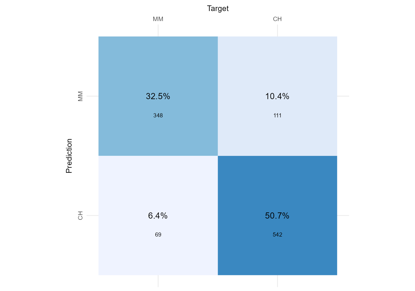> >Classifier 2

First, I calculate our total sample size from figure 1 by adding all data points together (I could also sum it from figure 2; the result should be the same). The total sample size is 1070:

sample_size = 348 + 111 + 69 + 542
sample_size

## [1] 1070

Then, I calculate the accuracy of both figures by summing the data points each model predicts correctly (.e.g., the model predicts MM when the true value is MM, and it predicts CH when the true value is CH) and divide that by the total sample size.

# Accuracy
accuracy_test_1 <- (348 + 542) /sample_size
cat("The accuracy of the model corresponding to figure 1 is", 
    sprintf("%.2f %%", accuracy_test_1*100), ". ", fill = TRUE)

## The accuracy of the model corresponding to figure 1 is 83.18 % .

accuracy_test_2 <- (307 + 559) /sample_size
cat("The accuracy of the model corresponding to figure 2 is", 
    sprintf("%.2f %%", accuracy_test_2*100), ". ", fill = TRUE)

## The accuracy of the model corresponding to figure 2 is 80.93 % .

As we do not have a preference for any particular brand, we will not calculate the specificity (true negative rate). The specificity would become relevant if we had a preference for predicting CH correctly (the “negative” value here). We could stop here and use accuracy as our final metric to evaluate model fit. Accuracy is the best metric to use when focusing on correctly identified variables (True Positives and True Negatives).

(It continues on the next tab ➡️)

On the other hand, the F1-score is the best metric to use when we focus on the incorrectly identified variables (False Negatives and False Positives). The question didn’t precisely indicate what rate the potential client was most interested in.

However, we know F1-score is a better metric if the class distribution is imbalanced. Thus, I will check the class distribution based on figure 1 (the total MM data points in the dataset (total_real_yes) and the total CH data points in the dataset (total_real_no)).

total_real_yes <- 348 + 69
total_real_no <- 111 + 542
total_real_yes/sample_size

    ## [1] 0.3897196

total_real_no/sample_size

## [1] 0.6102804

The class distribution is slightly imbalanced (39% of the total observed data points are MM, whereas 61% are CH). Thus I will choose to calculate the F1 scores for both models. To do so, I need to calculate the recall (true positive rate) and the precision (the rate of true positives from all the real positive).

Recall

Sensitivity or Recall: True Positive Rate

Figure 1

# Sensitivity or Recall: True Positive Rate
total_correct_yes_1 <- 348
TPR_test_1 <- total_correct_yes_1/total_real_yes
cat("The recall (true positive rate) of the model corresponding to figure 1 is", 
    sprintf("%.2f %%", TPR_test_1*100), ". ", fill = FALSE)

## The recall (true positive rate) of the model corresponding to figure 1 is 83.45 % .

Figure 2

total_correct_yes_2 <- 307
TPR_test_2 <- total_correct_yes_2/total_real_yes
cat("The recall (true positive rate) of the model corresponding to figure 2 is", 
    sprintf("%.2f %%", TPR_test_2*100), ".", fill = FALSE)

## The recall (true positive rate) of the model corresponding to figure 2 is 73.62 % .

Precision

Figure 1

## Precision: How many True Positives over all predicted="MM"? 
total_predicted_yes_1 <- 348 + 111
precision_test_1 <- total_correct_yes_1/total_predicted_yes_1
cat("The precision of the model corresponding to figure 1 is", 
    sprintf("%.2f %%", precision_test_1*100), ". ", fill = FALSE)

## The precision of the model corresponding to figure 1 is 75.82 % .

Figure 2

total_predicted_yes_2 <- 307 + 94
precision_test_2 <- total_correct_yes_2/total_predicted_yes_2
cat("The precision of the model corresponding to figure 2 is", 
    sprintf("%.2f %%", precision_test_2*100), ".", fill = FALSE)

## The precision of the model corresponding to figure 2 is 76.56 % .

F1-score

Figure 1

f1_test_1 <- (2*precision_test_1*TPR_test_1)/(precision_test_1 + TPR_test_1)
cat("The f1-score of the model corresponding to figure 1 is", 
    f1_test_1, ". ", fill = FALSE)

## The f1-score of the model corresponding to figure 1 is 0.7945205 .

Figure 2

f1_test_2 <- (2*precision_test_2*TPR_test_2)/(precision_test_2 + TPR_test_2)
cat("The f1-score of the model corresponding to figure 2 is", 
    f1_test_2, ".", fill = FALSE)

## The f1-score of the model corresponding to figure 2 is 0.7506112 .

(It continues on the next tab ➡️)

Based on our chosen metric, the f1-score, Classifier 1 is better at predicting Orange Juice Sales per brand as the f1-score is slightly higher than the f1-score for Classifier 2 (0.79 vs 0.75) ¹. If we had focused on accuracy, we would have had the same result; Classifier 1 predicts 83.18% of the values correctly as opposed to 80.93% for Classifier 2.

In “real life”, however, we would inspect more features of the model to reach our conclusion beyond the simple confusion matrix (e.g., the distribution of residuals).

📑 What we liked about this response

The question seemed easy at first. It seemed like the kind of thing accuracy could solve. This student was among the few who spotted the class imbalance in this dataset, reflected on it, and suggested an alternative metric.
It is a somewhat long response, yet it does not distract us from the question. Instead, it is well-structured, well-written, a joy to read, and thus easy to follow.
We also love that they used R code to illustrate their thinking process neatly.

Q3. Decision Trees (15 points)

Click to remember the question

For this question, we used the quanteda.textmodels::data_corpus_moviereviews corpus. This dataset consists of 2000 movie reviews and we have a target variable, called sentiment. The dataset is quite balanced, we have 1000 sentiment="yes" (indicating a positive sentiment towards the movie), the other 1000, sentiment="no", indicating a negative review.

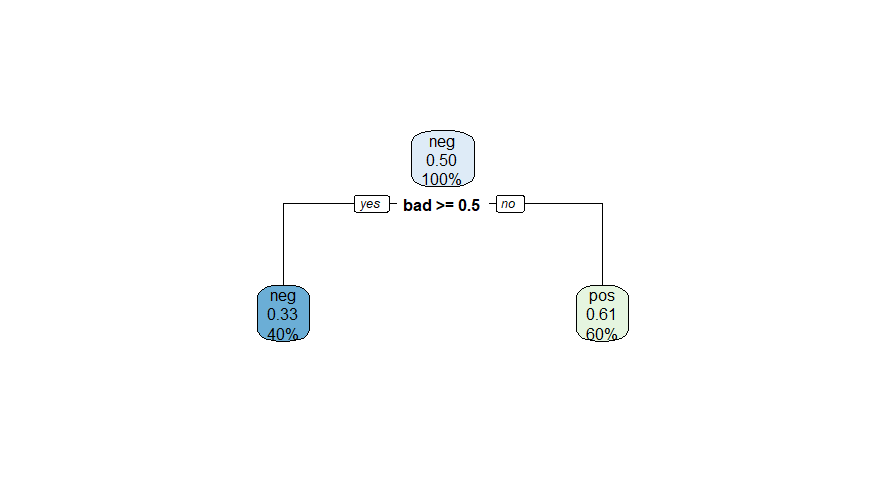
We trained two separate decision trees, one with tree_depth=1 and another with tree_depth=4, on this dataset. As you probably know, the figures below depicts the fitted trees, and it contains useful information about how well the models fit the training data. Here is what we want from you: based on the information contained in these figures, calculate the F1-score of each model for the target variable sentiment="yes", explain how you calculated the scores and indicate which of the two models performed better.

Decision Tree Model 1

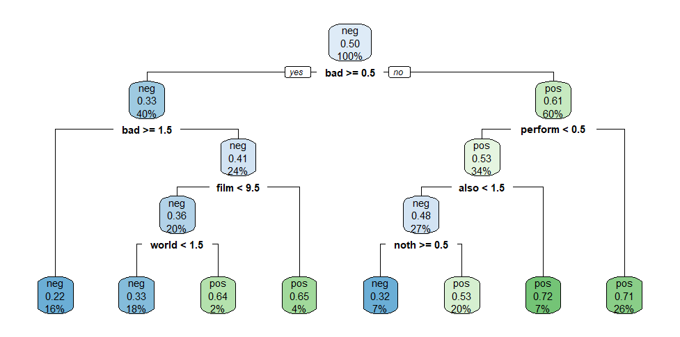
Decision Tree Model 2

To calculate f1-scores, I need to calculate the recall (true positive rate) and the precision (the rate of true positives from all the real positives).

From the explanation above, we know that the total number of real positive observations (sentiment="yes") is 1000, and the total sample size is 2000. Let’s store these values in variables.

total_real_yes_dt <- 1000
sample_size_dt <- 2000

For our calculation of recall and precision, we still need to extract the following information from our decision trees:

the number of all positively predicted values (the values that predict sentiment="yes", e.g., the sum of the true positives and false negatives) for our calculation of precision;
and the number of true positives (the values that predict sentiment="yes" and actually have a sentiment of “yes”)

Where to find this information?

We only need to focus on the tree’s leaf nodes to extract this information. In every node, there are three lines:

The first line contains ‘pos’ or ‘neg’, indicating which sentiment is predicted for all values in this node. ‘Pos’ indicates a prediction of sentiment="yes", and ‘neg’ indicates a prediction of sentiment="no".
- The node’s colour varies depending on this overall prediction, ‘pos’ nodes are different shades of green and ‘neg’ nodes are different shades of blue. Since we are focused on positively predicted values, we will focus on green ‘pos’ nodes;
The second line contains a number which is the probability of the values contained in that node to be ‘pos’ (e.g., to have a sentiment='yes')
The third line indicates the portion of the total data contained in that node.

In a decision tree, the values predicted at the end are shown in the leaf nodes (the deepest nodes of the tree). Thus, we will only focus on each tree’s green ‘pos’ end nodes.

(It continues on the next tab ➡️)

Calculating positively predicted values

First, we will calculate the sum of all positively predicted values. Because final predictions are contained in end nodes, and green ‘pos’ end nodes predict positive values for all the data points it contains, we can obtain the sum of all positively predicted values by adding the percentages of data points contained in green end nodes and multiplying this by our total sample size.

Figure 1

In the first decision tree, we only have one green end node containing 60% of the total data. Therefore:

total_predicted_yes_dt1 <- (60/100)*sample_size_dt
cat("In the first decision tree", total_predicted_yes_dt1, 
    "observations are predicted as sentiment='yes'.")

## In the first decision tree 1200 observations are predicted as sentiment='yes'.

Figure 2

Five green end nodes in the second decision tree contain 2%, 4%, 20%, 7% and 26% of the data in the second decision tree. Therefore:

total_predicted_yes_dt2 <- ((2/100)+(4/100)+(20/100)+(7/100)+(26/100))*sample_size_dt
cat("In the second decision tree", total_predicted_yes_dt2, 
    "observations are predicted as sentiment='yes'.")

## In the second decision tree 1180 observations are predicted as sentiment='yes'.

Sum of true positives

Secondly, we will calculate the sum of true positives. The number on the second line of each node effectively represents the true positive rate of that node.

It should be noted, however, that this is not the exact rate of true positives but just a rounded-up value of the probability of predicting a positive value in that node. Nevertheless, it approximates the true positive rate and is the best estimate we can find for this exercise. Thus from now on, we will call this probability the “true positive rate” of the node.

Thus, focusing on the same nodes as before, we will:

calculate the number of data points in each node by multiplying the third line percentage by the sample size
multiply the number found in step 1. for each node by its respective “true positive rate” from the second line,
sum all of these numbers together to have total true positives.

Figure 1

We still have one green end node in the first decision tree containing \(60%\) of the total data, with a “true positive rate” of \(0.61\):

total_correct_yes_dt1 <- ((60/100)*sample_size_dt)*0.61
cat("In the first decision tree", total_correct_yes_dt1, "observations are true positives.")

## In the first decision tree 732 observations are true positives.

Figure 2

In the second decision tree, we still have five green end nodes containing \(2%\), \(4%\), \(20%\), \(7%\) and \(26%\) of the total data, with respective “true positive rates” of \(0.64\), \(0.65\), \(0.53\), \(0.72\) and \(0.71\).

total_correct_yes_dt2 <- (
     ((2/100)*sample_size_dt)*0.64 + ((4/100)*sample_size_dt)*0.65 +
     ((20/100)*sample_size_dt)*0.53 + ((7/100)*sample_size_dt)*0.72 + ((26/100)*sample_size_dt)*0.71
)
cat("In the second decision tree", total_correct_yes_dt2, "observations are true positives.")

## In the second decision tree 759.6 observations are true positives.

(It continues on the next tab ➡️)

Now, we have all the information we need to calculate:

the recall (the true positive rate) obtained by dividing the true positive values by the sum of the true positives and false negatives;
the precision obtained by dividing the true positive values by the sum of the true positives and false positives;
and the f1-score, obtained by multiplying by 2 the division between the product of precision and recall and the sum of precision and recall.

Figure 1

# Sensitivity or Recall: True Positive Rate
TPR_test_dt1 <- total_correct_yes_dt1/total_real_yes_dt
cat("The recall (true positive rate) of the first decision tree is", 
    sprintf("%.2f %%", TPR_test_dt1*100), ". ", fill = FALSE)

## The recall (true positive rate) of the first decision tree is 73.20 % .

## Precision: How many True Positives over all predicted="yes"? 
precision_test_dt1 <- total_correct_yes_dt1/total_predicted_yes_dt1
cat("The precision of the first decision tree is", 
    sprintf("%.2f %%", precision_test_dt1*100), ". ", fill = FALSE)

## The precision of the first decision tree is 61.00 % .

f1_test_dt1 <- (2*precision_test_dt1*TPR_test_dt1)/(precision_test_dt1 + TPR_test_dt1)
cat("The f1-score of the first decision tree is", f1_test_dt1, ". ", fill = FALSE)

## The f1-score of the first decision tree is 0.6654545 .

Figure 2

TPR_test_dt2 <- total_correct_yes_dt2/total_real_yes_dt
cat("The recall (true positive rate) of the second decision tree is", 
    sprintf("%.2f %%", TPR_test_dt2*100), ". ", fill = FALSE)

## The recall (true positive rate) of the second decision tree is 75.96 % .

precision_test_dt2 <- total_correct_yes_dt2/total_predicted_yes_dt2
cat("The precision of the second decision tree is", 
    sprintf("%.2f %%", precision_test_dt2*100), ". ", fill = FALSE)

## The precision of the second decision tree is 64.37 % .

f1_test_dt2 <- (2*precision_test_dt2*TPR_test_dt2)/(precision_test_dt2 + TPR_test_dt2)
cat("The f1-score of the second decision tree is", f1_test_dt2, ". ", fill = FALSE)

## The f1-score of the second decision tree is 0.6968807 .

(It continues on the next tab ➡️)

Solely based on the f1-score, the second decision tree is better at predicting the sentiment towards the movie as the f1-score is slightly higher than the f1-score for the first decision tree (\(0.70\) vs \(0.67\)). ²

📑 What we liked about this response

The quality of the response speaks for itself. The author did a great job of explaining the concepts and the code in a way that is easy to follow, although this one could have been a bit shorter. (tabs are my addition, but the student used markdown-style bullet points, etc.)
As with the previous response, we love that the author used R code to illustrate their thinking process.

Footnotes

an f1-score can have values ranging from 0 to 1 and the best f1-score value possible is 1↩︎
an f1-score can have values ranging from 0 to 1, and the best f1-score value possible is 1.↩︎