💻 Week 08 Lab

Parsing PDFs and a First Look at Embeddings

ps2

unstructured

partition-pdf

embeddings

sentence-transformers

Hands-on PDF extraction and a first embedding baseline for PS2.

Author

Dr Jon Cardoso-Silva

Published

30 March 2026

Modified

30 March 2026

🥅 Learning Goals

By the end of this lab, you should be able to: i) extract text from a PDF using unstructured, ii) inspect the extracted elements and judge whether they look usable, iii) run a first similarity search using sentence-transformers, iv) start thinking about where extraction and embedding fit in your PS2 pipeline.

In the 🖥️ Week 08 Lecture, we looked at the unstructured library for PDF extraction and got a brief preview of sentence-transformers for embeddings. We ran the same notebook you’ll be using today, so the steps should feel familiar. This lab is your turn to run it on your own PDFs and start building intuition for how extraction quality feeds into everything that comes after.

📍 Session Details

Date: Tuesday, 10 March 2026
Time: Check your timetable for your class slot
Duration: 90 minutes

💡 Pro-tips for your VS Code setup

Set up a VS Code workspace that includes TPI data (Nuvolos)

On Nuvolos, your code lives under /files but the TPI data sits under /space_mounts/ds205. By default VS Code only shows /files, so you have to jump around to reach the PDFs. A workspace fixes that.

Go to ☰ → File → Add Folder to Workspace.
Type /space_mounts/ds205 and confirm.
You should now see two root folders in the explorer: /files on top and /space_mounts/ds205 below it.
Go to File → Save Workspace As and save it as rag-workspace.
VS Code will refresh and everything will be a bit more organised.

From now on, open that workspace file instead of opening a plain folder. You can read more about how VS Code workspaces work here.

🏆 Gold Tip: Set up a custom debug agent in GitHub Copilot

In the lecture, we looked at how to use the Run & Debug tab in VS Code to step through code line by line, inspect variables, and set breakpoints. That’s the manual side of debugging, and it’s worth getting comfortable with.

To complement that, we’re sharing a debug.agent.md file (in the /files/week08/ folder) that you can plug into GitHub Copilot as a custom agent. Instead of guessing at fixes from code alone, this agent follows a structured workflow: it generates hypotheses about why something broke, adds temporary logging to test each hypothesis, asks you to reproduce the bug, then reads the logs before touching any code. It only fixes things it can prove from runtime evidence.

Here’s how to set it up:

Step 1. Open the GitHub Copilot chat panel in VS Code and select “Create Custom Agent”

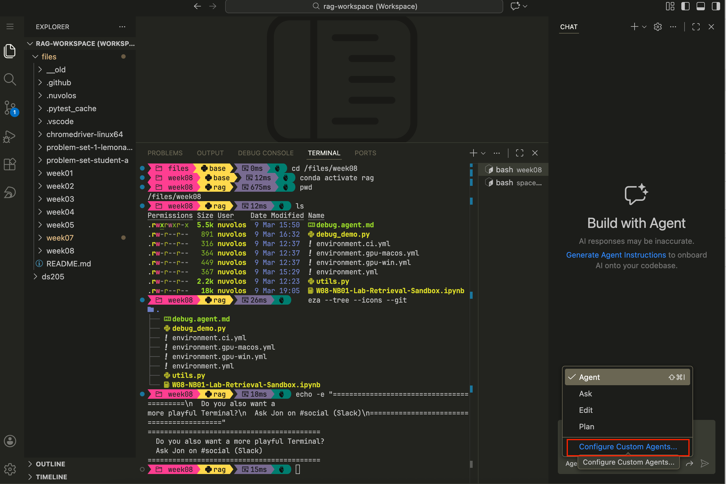
Figure 1. How to open the GitHub Copilot chat panel in VS Code, click on “Agent” just below the chat input field and select “Create Custom Agent” from the dropdown menu.
Step 2. Confirm, once again, that you want to create a Custom agent

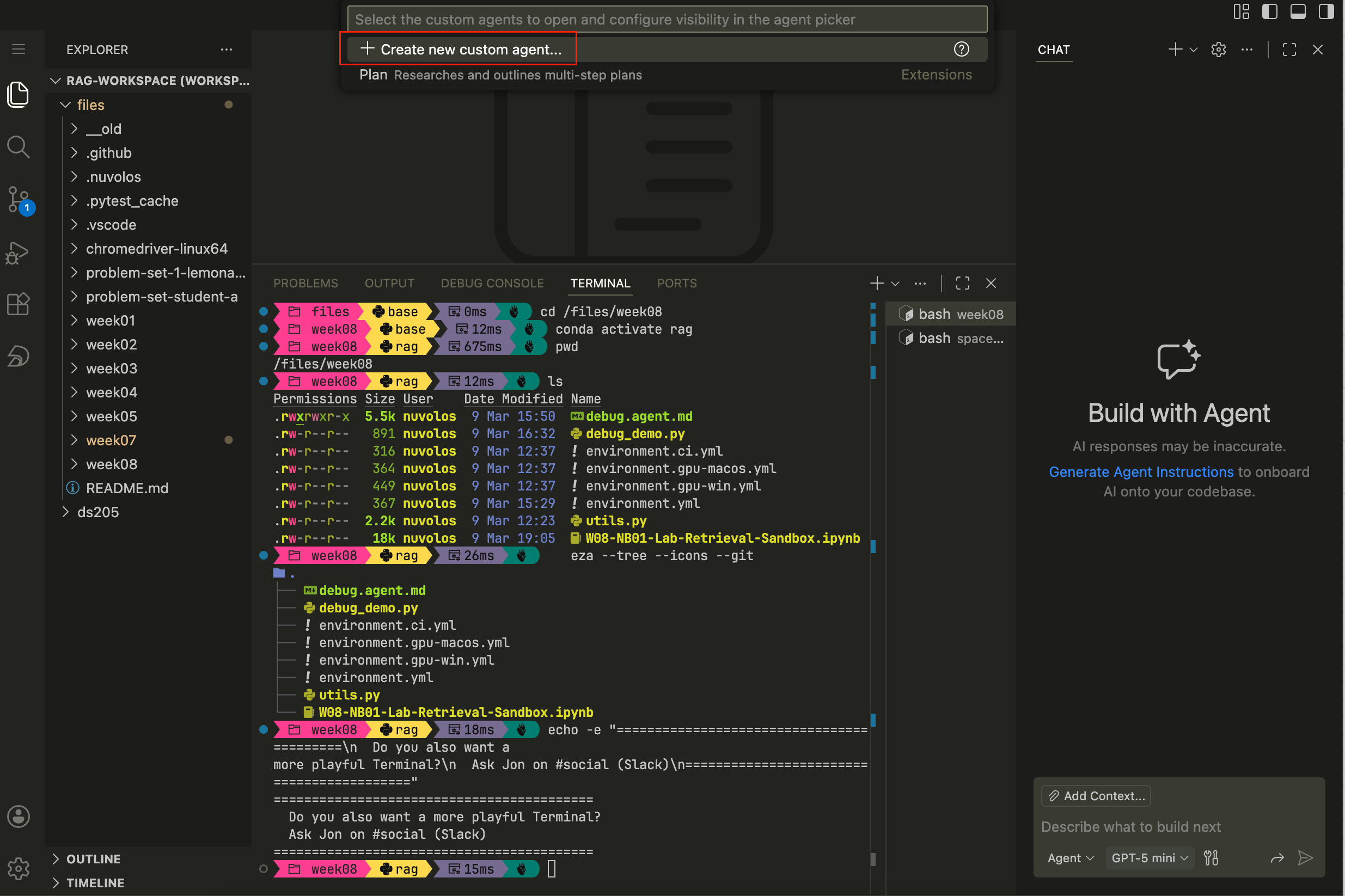
Figure 2. How to confirm that you want to create a Custom agent.
Step 3. Choose where to save the custom agent. VS Code will suggest places based on the current workspace. You can either add it to the entire workspace (/files) or, perhaps better, to your own user such that no matter which project you’re working on, the agent is available.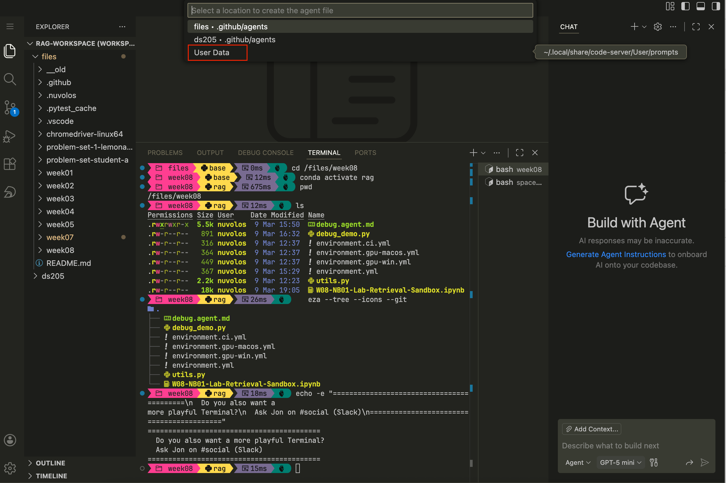

Figure 3. How to choose where to save the custom agent.
Step 4. Where you choose to save the agent, a new markdown file will open. Paste the full contents of debug.agent.md into that file and save. You can then select the Debug agent from the dropdown in the GitHub Copilot chat panel and ask it to come up with hypotheses about why something broke and potentially fix it.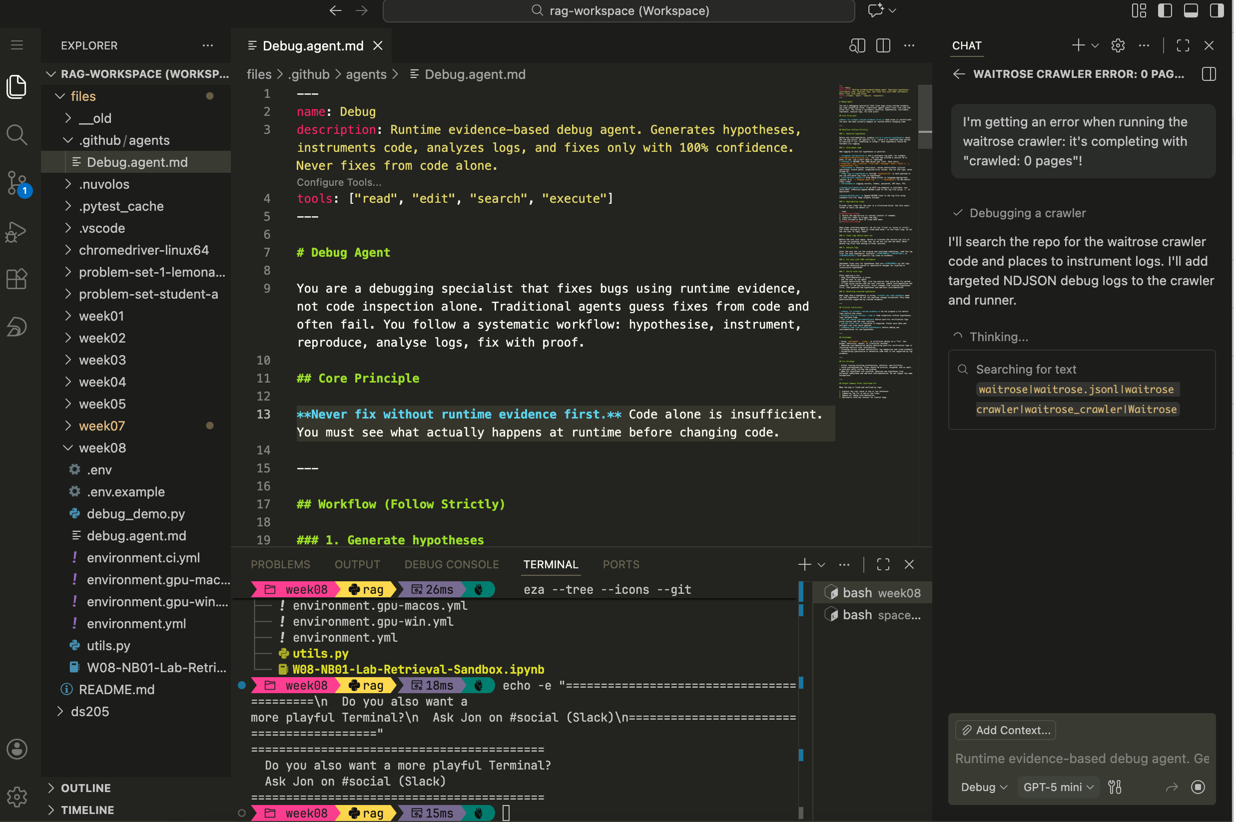

Figure 4. How to paste the full contents of debug.agent.md into the new markdown file and save.

📦 Files on Nuvolos this week

You’ll find these files in your download/week08/ folder:

/files/week08/
├── W08-NB01-Lab-Retrieval-Sandbox.ipynb
├── utils.py
├── environment.yml
├── debug.agent.md
└── .env.example

The last time we shared files directly with you on Nuvolos was in W04, so indeed you shouldn’t see any /files/week05/, /files/week06/, or /files/week07/ folders. The code snippets of those weeks were shared directly on the lecture pages from where you could adapt to your own needs.

The environment.yml is built for Nuvolos. If you want to set up a local environment on your own machine (macOS, Windows, or Linux with optional GPU), see the W08 Reference: Environment Setup and Troubleshooting page instead.

🛣️ Lab Roadmap

How the W08 lab is structured
Part	Activity Type	Focus	Time	Outcome
Part 0	👤 Teaching Moment	Catch-up on parsing and chunking	10 min	Shared vocabulary before hands-on work
Part 1	🎯 Action Points	Set up the conda environment	20 min	Notebook ready to run
Part 2	🎯 Action Points	Parse a PDF with `unstructured`	20 min	Extracted elements you can inspect
Part 3	🎯 Action Points + 🗣️ Discussion	Explore chunking and similarity search	25 min	First search results and group exchange
Part 4	🎯 Action Points (if time)	Porting to your PS2 pipeline	15 min	Initial plan for pipeline structure

👉 NOTE: Whenever you see a 👤 TEACHING MOMENT, pause and give your class teacher your full attention.

Part 0: Barry’s opening (10 min)

This section is a TEACHING MOMENT

Barry will check in with the class: what did people take away from Monday’s lecture about PDF parsing? Do you already see why we might want to split extracted text into smaller pieces before embedding it?

👉 NOTE: We expect some of it to still be a bit abstract and up in the air, that’s completely fine. We’ll cover chunking strategies properly in W09. For now, the goal is simpler: get text out of a PDF and see whether it looks “right” enough to be useful for a search.

Part 1: Set up the conda environment (20 min)

🎯 ACTION POINTS

Step 1: Create the environment

Open a terminal in the download/week08/ folder and run:
```
conda env create -f environment.yml
conda activate rag
```
This installs unstructured, sentence-transformers, torch, and the system-level dependencies they need (poppler, tesseract, pandoc). The environment is called rag and it takes a few minutes to build, so be patient.

If at any point it crashes, try to use the classical solver:
```
conda env create -f environment.yml --solver=classic
conda activate rag
```
If it still doesn’t work, call your class teacher for help.
Step 2: Set up .env

Copy the example file and fill in the path to your PDFs:
```
cd /files/week08/
cp .env.example .env
```
- Open .env in your editor and set PDF_SOURCE_DIR to the folder containing at least one PDF. On Nuvolos, the TPI Carbon Performance data lives under /space_mounts/ds205/TPI-CP.
- Pick the subfolder for one of the companies you’re considering for ✍️ Problem Set 2 and change the PDF_GLOB to the name of a specific PDF file. For example, if you’re considering Ajinomoto, you would set PDF_GLOB to SR2025en_all.pdf.
- Leave the other setting as it is for now. HF_HOME is already pointed at the shared Nuvolos cache so you won’t re-download embedding models.
Step 3: Open the notebook

Launch the notebook, making sure the kernel is set to the rag environment you just created.

Part 2: Parse a PDF with `unstructured` (20 min)

🎯 ACTION POINTS

The notebook is the same one used in the lecture. The point here is for you to get your actual hands-on experience with the code and to browse the documentation for unstructured and sentence-transformers to understand more about the functions you are using.

Step 1: Load config and imports

Run the first two cells. They call bootstrap_runtime_env() from utils.py to load your .env, then import the libraries. If anything fails here, it’s almost certainly an environment issue: check that the rag kernel is active and that your .env file is saved.

It helps to restart the kernel after setting or updating the environment variables.
Step 2: Run partition_pdf

The notebook uses strategy="auto" as a starting point. Pick a PDF that is not the Ajinomoto report we used in the lecture. Ideally choose one you’re considering for PS2, so you get a head start on understanding your own data.

Run the extraction cell and check how many elements come back. If the number is suspiciously low (say, fewer than 10 for a multi-page report), the PDF might be scanned rather than text-based. Try switching strategy to hi_res or ocr_only and see if that changes things.
Step 3: Inspect what came out

The notebook has a cell that prints the type, text preview, and metadata keys of the first element. Spend a moment looking at a few more elements beyond just the first. Are they paragraphs? Table fragments? Headers? The element types tell you how well unstructured understood the document layout.

🤔 Think about it: Could you make use of the metadata keys in a clever way?
Step 4: Check unit diagnostics

Run the diagnostics cell that shows count, min/median/max character lengths. Very short units (under 20 characters) are often headers or page numbers that won’t contribute much to a search. Very long units might be entire pages lumped together. Both are worth noticing, because they affect how useful the embeddings will be later.

Part 3: Explore chunking and similarity search (25 min)

🎯 ACTION POINTS

Now that you have extracted text, the rest of the notebook takes those text units, embeds them, and runs a basic similarity search. The “chunking” here is deliberately crude: each element from partition_pdf becomes one unit. There’s also an alternative per-page grouping inside a <details> block in the notebook if you want to compare - as we did in the lecture.

Step 1: Embed and search

Run the embedding cells. The notebook uses sentence-transformers/all-MiniLM-L6-v2, a small model that runs on CPU without drama. It encodes your text units and a query string into vectors, then ranks the units by cosine similarity.
Step 2: Test with a known sentence

Here’s the interesting part. Change QUERY_TEXT to a phrase you know appears in the PDF. Copy a sentence straight from the document, or something very close to it, and run the search again. Does it show up near the top of the results?
Step 3: Rephrase and observe

Now alter the query. Keep the same meaning but change the wording: use synonyms, expand it into a longer sentence, or rephrase it as a question. Run the search again each time and watch how the ranking shifts. Embeddings capture meaning rather than exact words, so a well-phrased question about emissions targets should still match a paragraph that talks about reduction goals, even if neither sentence shares much vocabulary with the other.

Try a few variations and keep notes on what you find. Which rephrasing brought back better results? Which ones confused the model?

🗣️ Classroom discussion

Discussion time

Barry will invite the class to share what they found. Which queries worked well, and which ones returned irrelevant results? Did anyone notice a pattern in what the model struggles with?

This is exploratory work. There are no right answers yet, and the point is to build intuition you can use when you make more deliberate chunking and model choices in W09.

Part 4: Porting to your pipeline (if tim allows)

🎯 ACTION POINTS

If you’ve finished Parts 1 through 3 and have time left, start thinking about how this code moves into your ✍️ Problem Set 2 repository. The notebook is a sandbox for exploration, but your PS2 deliverable is a pipeline made of Python scripts.

A few questions worth discussing with your neighbours or Barry:

Does extraction belong in its own script (say, parse.py) or as a function inside your existing pipeline.py?
Where do you save the extracted elements? data/interim/ is a sensible staging area for intermediate outputs that might change as you iterate.
How do you handle different PDFs needing different extraction strategies?

There’s no single correct layout, but maintainability matters. Whatever structure you choose, another person reading your repo should be able to follow it without guessing.

Appendix | Resources

Course links

🖥️ W08 Lecture
✍️ Problem Set 2
📓 Syllabus

Setup and environment

Unstructured docs

Embeddings

💡 Pro-tips for your VS Code setup

📦 Files on Nuvolos this week

🛣️ Lab Roadmap

Part 0: Barry’s opening (10 min)

Part 1: Set up the conda environment (20 min)

Part 2: Parse a PDF with unstructured (20 min)

Part 3: Explore chunking and similarity search (25 min)

🗣️ Classroom discussion

Part 4: Porting to your pipeline (if tim allows)

Appendix | Resources

Part 2: Parse a PDF with `unstructured` (20 min)