
DS101A Week 03 - Exploratory Data Analysis Notebook
The content below recaps the content of the exploratory data analysis demo from the Week 03 lecture. The demo explored a dataset from Kaggle about inflation rates across 206 countries from 1970 to 2022.
Click on the button below to download the source files (.csv dataset and .ipynb notebook) that were used to create this page, if you ever want to try the demo for yourselves:
(this is a zip file because there are source code files in it)
Python library imports
For the purposes of this analysis, we are importing the “usual suspect” libraries for data and string manipulation (i.e pandas, numpy and re), path manipulation (os and glob) but also a whole host of libraries for visualisation and a library for time series modeling/forecasting (statsmodels.tsa.arima.model).
#library for the manipulation of dates
import datetime
# library for the manipulation of strings
import re
# libraries for the manipulation of data (data frames)
import pandas as pd
import numpy as np
# libraries for the manipulation of (file) paths
import os
import glob
# libraries for visualisation and plotting
import matplotlib.pyplot as plt
import seaborn as sns
import plotly.graph_objects as go
import plotly.subplots as sp
import plotly.graph_objs as go
from IPython.display import display_html
# library for time series modelling
from statsmodels.tsa.arima.model import ARIMA
Reading the data file
f='Global_Dataset_of_Inflation.csv'
df = pd.read_csv(f)
---------------------------------------------------------------------------
UnicodeDecodeError Traceback (most recent call last)
File /Users/g.berrada/DS101/2023-2024/autumn-term/weeks/week03/python_notebook/eda.qmd:2
1 f='Global_Dataset_of_Inflation.csv'
----> 2 df = pd.read_csv(f)
File /opt/anaconda3/lib/python3.12/site-packages/pandas/io/parsers/readers.py:1026, in read_csv(filepath_or_buffer, sep, delimiter, header, names, index_col, usecols, dtype, engine, converters, true_values, false_values, skipinitialspace, skiprows, skipfooter, nrows, na_values, keep_default_na, na_filter, verbose, skip_blank_lines, parse_dates, infer_datetime_format, keep_date_col, date_parser, date_format, dayfirst, cache_dates, iterator, chunksize, compression, thousands, decimal, lineterminator, quotechar, quoting, doublequote, escapechar, comment, encoding, encoding_errors, dialect, on_bad_lines, delim_whitespace, low_memory, memory_map, float_precision, storage_options, dtype_backend)
1013 kwds_defaults = _refine_defaults_read(
1014 dialect,
1015 delimiter,
(...)
1022 dtype_backend=dtype_backend,
1023 )
1024 kwds.update(kwds_defaults)
-> 1026 return _read(filepath_or_buffer, kwds)
File /opt/anaconda3/lib/python3.12/site-packages/pandas/io/parsers/readers.py:620, in _read(filepath_or_buffer, kwds)
617 _validate_names(kwds.get("names", None))
619 # Create the parser.
--> 620 parser = TextFileReader(filepath_or_buffer, **kwds)
622 if chunksize or iterator:
623 return parser
File /opt/anaconda3/lib/python3.12/site-packages/pandas/io/parsers/readers.py:1620, in TextFileReader.__init__(self, f, engine, **kwds)
1617 self.options["has_index_names"] = kwds["has_index_names"]
1619 self.handles: IOHandles | None = None
-> 1620 self._engine = self._make_engine(f, self.engine)
File /opt/anaconda3/lib/python3.12/site-packages/pandas/io/parsers/readers.py:1898, in TextFileReader._make_engine(self, f, engine)
1895 raise ValueError(msg)
1897 try:
-> 1898 return mapping[engine](f, **self.options)
1899 except Exception:
1900 if self.handles is not None:
File /opt/anaconda3/lib/python3.12/site-packages/pandas/io/parsers/c_parser_wrapper.py:93, in CParserWrapper.__init__(self, src, **kwds)
90 if kwds["dtype_backend"] == "pyarrow":
91 # Fail here loudly instead of in cython after reading
92 import_optional_dependency("pyarrow")
---> 93 self._reader = parsers.TextReader(src, **kwds)
95 self.unnamed_cols = self._reader.unnamed_cols
97 # error: Cannot determine type of 'names'
File parsers.pyx:574, in pandas._libs.parsers.TextReader.__cinit__()
File parsers.pyx:663, in pandas._libs.parsers.TextReader._get_header()
File parsers.pyx:874, in pandas._libs.parsers.TextReader._tokenize_rows()
File parsers.pyx:891, in pandas._libs.parsers.TextReader._check_tokenize_status()
File parsers.pyx:2053, in pandas._libs.parsers.raise_parser_error()
File <frozen codecs>:322, in decode(self, input, final)
UnicodeDecodeError: 'utf-8' codec can't decode byte 0xf4 in position 12550: invalid continuation byteA first try at reading the .csv file that contains the dataset results in an error that shows that the file is not encoded in the default UTF-8 format (the pandas read_csv function expects an UTF-8 encoding by default). A quick analysis of the error message shows that the file is in fact encoded in ISO-8859-1 format, so we’ll have to pass an optional encoding argument to read_csv to allow it to read the file correctly.
df = pd.read_csv('Global_Dataset_of_Inflation.csv',encoding='ISO-8859-1')
df| Country Code | IMF Country Code | Country | Indicator Type | Series Name | 1970 | 1971 | 1972 | 1973 | 1974 | … | 2019 | 2020 | 2021 | 2022 | Note | Unnamed: 59 | Unnamed: 60 | Unnamed: 61 | Unnamed: 62 | Unnamed: 63 | |
|---|---|---|---|---|---|---|---|---|---|---|---|---|---|---|---|---|---|---|---|---|---|
| 0 | ABW | 314.0 | Aruba | Inflation | Headline Consumer Price Inflation | NaN | NaN | NaN | NaN | NaN | … | 4.26 | 1.22 | 0.74 | 6.04 | Annual average inflation | NaN | NaN | NaN | NaN | NaN |
| 1 | AFG | 512.0 | Afghanistan | Inflation | Headline Consumer Price Inflation | 25.51 | 25.51 | -12.52 | -10.68 | 10.23 | … | 2.30 | 5.44 | 5.06 | NaN | Annual average inflation | NaN | NaN | NaN | NaN | NaN |
| 2 | AGO | 614.0 | Angola | Inflation | Headline Consumer Price Inflation | 7.97 | 5.78 | 15.80 | 15.67 | 27.42 | … | 17.08 | 21.02 | 23.85 | 21.35 | Annual average inflation | NaN | NaN | NaN | NaN | NaN |
| 3 | ALB | 914.0 | Albania | Inflation | Headline Consumer Price Inflation | NaN | NaN | NaN | NaN | NaN | … | 1.41 | 1.62 | 2.04 | 6.73 | Annual average inflation | NaN | NaN | NaN | NaN | NaN |
| 4 | ARE | 466.0 | United Arab Emirates | Inflation | Headline Consumer Price Inflation | 21.98 | 21.98 | 21.98 | 21.98 | 21.98 | … | -1.93 | -2.08 | 0.18 | 5.22 | Annual average inflation | NaN | NaN | NaN | NaN | NaN |
| … | … | … | … | … | … | … | … | … | … | … | … | … | … | … | … | … | … | … | … | … | … |
| 778 | VEN | 299.0 | Venezuela, RB | Inflation | Producer Price Inflation | NaN | NaN | NaN | NaN | NaN | … | NaN | NaN | NaN | NaN | Producer Price Index, All Commodities | NaN | NaN | NaN | NaN | NaN |
| 779 | VNM | 582.0 | Vietnam | Inflation | Producer Price Inflation | NaN | NaN | NaN | NaN | NaN | … | NaN | NaN | NaN | NaN | Producer Price Index, All Commodities | NaN | NaN | NaN | NaN | NaN |
| 780 | XKX | 967.0 | Kosovo | Inflation | Producer Price Inflation | NaN | NaN | NaN | NaN | NaN | … | 0.93 | -0.58 | 4.92 | NaN | Producer Price Index, All Commodities | NaN | NaN | NaN | NaN | NaN |
| 781 | ZAF | 199.0 | South Africa | Inflation | Producer Price Inflation | NaN | 5.00 | 6.35 | 12.44 | 18.58 | … | 4.62 | 2.49 | 7.12 | 14.36 | Producer Price Index, All Commodities | NaN | NaN | NaN | NaN | NaN |
| 782 | ZMB | 754.0 | Zambia | Inflation | Producer Price Inflation | 14.29 | 0.00 | 4.17 | 12.00 | 10.71 | … | NaN | NaN | NaN | NaN | Producer Price Index, All Commodities | NaN | NaN | NaN | NaN | NaN |
783 rows × 64 columns
Exploring the dataframe
We start by printing the first few rows of our dataframe (the first 5 by default) to get a sense of what our dataset looks like.
print(df.head())Country Code IMF Country Code Country Indicator Type \
0 ABW 314.0 Aruba Inflation
1 AFG 512.0 Afghanistan Inflation
2 AGO 614.0 Angola Inflation
3 ALB 914.0 Albania Inflation
4 ARE 466.0 United Arab Emirates Inflation
Series Name 1970 1971 1972 1973 1974 ... \
0 Headline Consumer Price Inflation NaN NaN NaN NaN NaN ...
1 Headline Consumer Price Inflation 25.51 25.51 -12.52 -10.68 10.23 ...
2 Headline Consumer Price Inflation 7.97 5.78 15.80 15.67 27.42 ...
3 Headline Consumer Price Inflation NaN NaN NaN NaN NaN ...
4 Headline Consumer Price Inflation 21.98 21.98 21.98 21.98 21.98 ...
2019 2020 2021 2022 Note Unnamed: 59 \
0 4.26 1.22 0.74 6.04 Annual average inflation NaN
1 2.30 5.44 5.06 NaN Annual average inflation NaN
2 17.08 21.02 23.85 21.35 Annual average inflation NaN
3 1.41 1.62 2.04 6.73 Annual average inflation NaN
4 -1.93 -2.08 0.18 5.22 Annual average inflation NaN
Unnamed: 60 Unnamed: 61 Unnamed: 62 Unnamed: 63
0 NaN NaN NaN NaN
1 NaN NaN NaN NaN
2 NaN NaN NaN NaN
3 NaN NaN NaN NaN
4 NaN NaN NaN NaN
[5 rows x 64 columns]We use the describe command to get some basic statistics about our dataframe.
df.describe()And we print out the dataframe column names.
df.columns| IMF Country Code | 1970 | 1971 | 1972 | 1973 | 1974 | 1975 | 1976 | 1977 | 1978 | … | 2017 | 2018 | 2019 | 2020 | 2021 | 2022 | Unnamed: 60 | Unnamed: 61 | Unnamed: 62 | Unnamed: 63 | |
|---|---|---|---|---|---|---|---|---|---|---|---|---|---|---|---|---|---|---|---|---|---|
| count | 781.000000 | 422.000000 | 428.000000 | 430.000000 | 430.000000 | 434.000000 | 434.000000 | 430.000000 | 427.000000 | 428.000000 | … | 737.000000 | 737.000000 | 728.000000 | 719.000000 | 706.000000 | 665.000000 | 0.0 | 0.0 | 0.0 | 0.0 |
| mean | 536.507042 | 5.867854 | 6.057173 | 7.705721 | 14.538465 | 24.174101 | 16.539424 | 15.472047 | 15.123021 | 12.062360 | … | 7.263428 | 503.428544 | 80.269581 | 36.131405 | 16.324632 | 17.285654 | NaN | NaN | NaN | NaN |
| std | 271.783250 | 7.283523 | 8.617909 | 11.701059 | 28.889492 | 39.117175 | 28.749170 | 37.833455 | 27.881710 | 18.019203 | … | 41.968311 | 7659.291543 | 1183.454979 | 649.033623 | 107.667579 | 32.234102 | NaN | NaN | NaN | NaN |
| min | 111.000000 | -26.098150 | -19.700000 | -12.520000 | -13.240000 | -35.940000 | -42.670000 | -10.900000 | -22.020000 | -23.800000 | … | -13.310000 | -14.400000 | -16.360000 | -31.430000 | -5.080000 | -1.970000 | NaN | NaN | NaN | NaN |
| 25% | 283.000000 | 1.640000 | 1.900000 | 3.015000 | 6.000000 | 11.355000 | 7.257500 | 4.900000 | 6.090000 | 4.375000 | … | 1.120000 | 1.270000 | 0.687500 | 0.100000 | 1.730000 | 5.450000 | NaN | NaN | NaN | NaN |
| 50% | 546.000000 | 4.360000 | 4.695000 | 5.590000 | 9.930000 | 17.545000 | 12.310000 | 9.585000 | 10.120000 | 8.285000 | … | 2.450000 | 2.490000 | 2.065000 | 1.880000 | 4.255000 | 9.110000 | NaN | NaN | NaN | NaN |
| 75% | 732.000000 | 7.670000 | 7.625000 | 8.775000 | 15.900000 | 28.260000 | 18.677500 | 15.975000 | 15.550000 | 12.925000 | … | 5.420000 | 4.810000 | 4.300000 | 4.170000 | 8.907500 | 17.530000 | NaN | NaN | NaN | NaN |
| max | 968.000000 | 61.000000 | 94.500000 | 115.200000 | 376.500000 | 513.700000 | 374.740000 | 510.700000 | 458.600000 | 175.510000 | … | 905.660000 | 169201.780000 | 19906.020000 | 17087.720000 | 1934.560000 | 433.190000 | NaN | NaN | NaN | NaN |
8 rows × 58 columns
From this initial exploration, we see that we have some rather uninteresting non-descript columns (the Unnamed : 59,…Unnamed : 63 columns), plenty of missing values to take care of (NaN values) and also that we will need to do some column name processing (many column names have spaces in them, which can be awkward to deal with when querying in particular).
Processing the dataframe to remove unnecessary columns and format the names of retained columns appropriately
We start by writing a function to process the previous dataframe to remove all unnecessary columns (i.e all Unnamed : x columns where x is a number between 59 and 63) and format the names of the columns we retain appropriately (i.e replace all spaces and special characters in column names by underscores and make all column names lowercase).
def import_and_process_csv(csv_file_path):
    """
    This function reads a CSV file, processes the column names by converting them to lowercase, replacing spaces
    with underscores, replacing special characters with underscores, and removing the specified 'Unnamed' columns.

    Args:
        csv_file_path (str): The path to the CSV file.

    Returns:
        pd.DataFrame: The processed DataFrame.
    """

    # Read the data from the CSV file into a DataFrame
    data = pd.read_csv(csv_file_path, encoding='ISO-8859-1')

    # Convert column names to lowercase
    data.columns = [col.lower() for col in data.columns]

    # Replace spaces with underscores (_)
    data.columns = [col.replace(' ', '_') for col in data.columns]

    # Replace special characters with underscores (_)
    data.columns = [re.sub(r'\W+', '_', col) for col in data.columns]

    # Remove the specified 'Unnamed' columns
    columns_to_remove = ['unnamed__59', 'unnamed__60', 'unnamed__61', 'unnamed__62', 'unnamed__63']
    data = data.drop(columns_to_remove, axis=1, errors='ignore')

    return data

data=import_and_process_csv(f)
data| country_code | imf_country_code | country | indicator_type | series_name | 1970 | 1971 | 1972 | 1973 | 1974 | … | 2014 | 2015 | 2016 | 2017 | 2018 | 2019 | 2020 | 2021 | 2022 | note | |
|---|---|---|---|---|---|---|---|---|---|---|---|---|---|---|---|---|---|---|---|---|---|
| 0 | ABW | 314.0 | Aruba | Inflation | Headline Consumer Price Inflation | NaN | NaN | NaN | NaN | NaN | … | 0.42 | 0.48 | -0.89 | -0.47 | 3.58 | 4.26 | 1.22 | 0.74 | 6.04 | Annual average inflation |
| 1 | AFG | 512.0 | Afghanistan | Inflation | Headline Consumer Price Inflation | 25.51 | 25.51 | -12.52 | -10.68 | 10.23 | … | 4.67 | -0.66 | 4.38 | 4.98 | 0.63 | 2.30 | 5.44 | 5.06 | NaN | Annual average inflation |
| 2 | AGO | 614.0 | Angola | Inflation | Headline Consumer Price Inflation | 7.97 | 5.78 | 15.80 | 15.67 | 27.42 | … | 7.30 | 9.16 | 32.38 | 29.84 | 19.63 | 17.08 | 21.02 | 23.85 | 21.35 | Annual average inflation |
| 3 | ALB | 914.0 | Albania | Inflation | Headline Consumer Price Inflation | NaN | NaN | NaN | NaN | NaN | … | 1.62 | 1.91 | 1.29 | 1.99 | 2.03 | 1.41 | 1.62 | 2.04 | 6.73 | Annual average inflation |
| 4 | ARE | 466.0 | United Arab Emirates | Inflation | Headline Consumer Price Inflation | 21.98 | 21.98 | 21.98 | 21.98 | 21.98 | … | 2.34 | 4.07 | 1.62 | 1.97 | 3.06 | -1.93 | -2.08 | 0.18 | 5.22 | Annual average inflation |
| … | … | … | … | … | … | … | … | … | … | … | … | … | … | … | … | … | … | … | … | … | … |
| 778 | VEN | 299.0 | Venezuela, RB | Inflation | Producer Price Inflation | NaN | NaN | NaN | NaN | NaN | … | 60.47 | 142.03 | 291.62 | 905.66 | 169201.78 | NaN | NaN | NaN | NaN | Producer Price Index, All Commodities |
| 779 | VNM | 582.0 | Vietnam | Inflation | Producer Price Inflation | NaN | NaN | NaN | NaN | NaN | … | 3.26 | -0.59 | -0.61 | NaN | NaN | NaN | NaN | NaN | NaN | Producer Price Index, All Commodities |
| 780 | XKX | 967.0 | Kosovo | Inflation | Producer Price Inflation | NaN | NaN | NaN | NaN | NaN | … | 1.63 | 2.66 | -0.07 | 0.59 | 1.35 | 0.93 | -0.58 | 4.92 | NaN | Producer Price Index, All Commodities |
| 781 | ZAF | 199.0 | South Africa | Inflation | Producer Price Inflation | NaN | 5.00 | 6.35 | 12.44 | 18.58 | … | 7.40 | 3.61 | 7.08 | 4.88 | 5.45 | 4.62 | 2.49 | 7.12 | 14.36 | Producer Price Index, All Commodities |
| 782 | ZMB | 754.0 | Zambia | Inflation | Producer Price Inflation | 14.29 | 0.00 | 4.17 | 12.00 | 10.71 | … | NaN | NaN | NaN | NaN | NaN | NaN | NaN | NaN | NaN | Producer Price Index, All Commodities |
783 rows × 59 columns
data.head(5)| country_code | imf_country_code | country | indicator_type | series_name | 1970 | 1971 | 1972 | 1973 | 1974 | … | 2014 | 2015 | 2016 | 2017 | 2018 | 2019 | 2020 | 2021 | 2022 | note | |
|---|---|---|---|---|---|---|---|---|---|---|---|---|---|---|---|---|---|---|---|---|---|
| 0 | ABW | 314.0 | Aruba | Inflation | Headline Consumer Price Inflation | NaN | NaN | NaN | NaN | NaN | … | 0.42 | 0.48 | -0.89 | -0.47 | 3.58 | 4.26 | 1.22 | 0.74 | 6.04 | Annual average inflation |
| 1 | AFG | 512.0 | Afghanistan | Inflation | Headline Consumer Price Inflation | 25.51 | 25.51 | -12.52 | -10.68 | 10.23 | … | 4.67 | -0.66 | 4.38 | 4.98 | 0.63 | 2.30 | 5.44 | 5.06 | NaN | Annual average inflation |
| 2 | AGO | 614.0 | Angola | Inflation | Headline Consumer Price Inflation | 7.97 | 5.78 | 15.80 | 15.67 | 27.42 | … | 7.30 | 9.16 | 32.38 | 29.84 | 19.63 | 17.08 | 21.02 | 23.85 | 21.35 | Annual average inflation |
| 3 | ALB | 914.0 | Albania | Inflation | Headline Consumer Price Inflation | NaN | NaN | NaN | NaN | NaN | … | 1.62 | 1.91 | 1.29 | 1.99 | 2.03 | 1.41 | 1.62 | 2.04 | 6.73 | Annual average inflation |
| 4 | ARE | 466.0 | United Arab Emirates | Inflation | Headline Consumer Price Inflation | 21.98 | 21.98 | 21.98 | 21.98 | 21.98 | … | 2.34 | 4.07 | 1.62 | 1.97 | 3.06 | -1.93 | -2.08 | 0.18 | 5.22 | Annual average inflation |
5 rows × 59 columns
Creating a continent column in the data dataframe after defining a country to continent mapping
We first create a dictionary that maps the country_code value to a continent value then use it to create a new continent column in our data dataframe.
# Define the mapping of country_code to continent
country_code_to_continent = {
    'AUS': 'Oceania',
    'AUT': 'Europe',
    'BEL': 'Europe',
    'BGR': 'Europe',
    'BLR': 'Europe',
    'BRA': 'South America',
    'CAN': 'North America',
    'CHE': 'Europe',
    'CHL': 'South America',
    'CHN': 'Asia',
    'COL': 'South America',
    'CRI': 'North America',
    'CYP': 'Asia',
    'CZE': 'Europe',
    'DEU': 'Europe',
    'DNK': 'Europe',
    'EGY': 'Africa',
    'ESP': 'Europe',
    'ETH': 'Africa',
    'FIN': 'Europe',
    'FRA': 'Europe',
    'GBR': 'Europe',
    'GHA': 'Africa',
    'GRC': 'Europe',
    'GTM': 'North America',
    'HUN': 'Europe',
    'IND': 'Asia',
    'IRL': 'Europe',
    'IRN': 'Asia',
    'ISL': 'Europe',
    'ISR': 'Asia',
    'ITA': 'Europe',
    'JOR': 'Asia',
    'JPN': 'Asia',
    'KOR': 'Asia',
    'KWT': 'Asia',
    'LKA': 'Asia',
    'LUX': 'Europe',
    'MAR': 'Africa',
    'MEX': 'North America',
    'MLT': 'Europe',
    'MUS': 'Africa',
    'MYS': 'Asia',
    'NIC': 'North America',
    'NLD': 'Europe',
    'NOR': 'Europe',
    'NZL': 'Oceania',
    'OMN': 'Asia',
    'PER': 'South America',
    'PHL': 'Asia',
    'POL': 'Europe',
    'PRT': 'Europe',
    'PRY': 'South America',
    'QAT': 'Asia',
    'ROU': 'Europe',
    'RUS': 'Europe',
    'RWA': 'Africa',
    'SAU': 'Asia',
    'SDN': 'Africa',
    'SEN': 'Africa',
    'SGP': 'Asia',
    'SLV': 'North America',
    'SVN': 'Europe',
    'SWE': 'Europe',
    'THA': 'Asia',
    'TTO': 'North America',
    'TUN': 'Africa',
    'TUR': 'Europe',
    'UGA': 'Africa',
    'UKR': 'Europe',
    'URY': 'South America',
    'USA': 'North America',
    'VEN': 'South America',
    'VNM': 'Asia',
    'ZAF': 'Africa'
}

# Create a new 'continent' column based on the 'country_code' column using the mapping defined above
data['continent'] = data['country_code'].map(country_code_to_continent)

# Print the first 5 rows of the DataFrame to verify the changes
data.head()| country_code | imf_country_code | country | indicator_type | series_name | 1970 | 1971 | 1972 | 1973 | 1974 | … | 2015 | 2016 | 2017 | 2018 | 2019 | 2020 | 2021 | 2022 | note | continent | |
|---|---|---|---|---|---|---|---|---|---|---|---|---|---|---|---|---|---|---|---|---|---|
| 0 | ABW | 314.0 | Aruba | Inflation | Headline Consumer Price Inflation | NaN | NaN | NaN | NaN | NaN | … | 0.48 | -0.89 | -0.47 | 3.58 | 4.26 | 1.22 | 0.74 | 6.04 | Annual average inflation | NaN |
| 1 | AFG | 512.0 | Afghanistan | Inflation | Headline Consumer Price Inflation | 25.51 | 25.51 | -12.52 | -10.68 | 10.23 | … | -0.66 | 4.38 | 4.98 | 0.63 | 2.30 | 5.44 | 5.06 | NaN | Annual average inflation | NaN |
| 2 | AGO | 614.0 | Angola | Inflation | Headline Consumer Price Inflation | 7.97 | 5.78 | 15.80 | 15.67 | 27.42 | … | 9.16 | 32.38 | 29.84 | 19.63 | 17.08 | 21.02 | 23.85 | 21.35 | Annual average inflation | NaN |
| 3 | ALB | 914.0 | Albania | Inflation | Headline Consumer Price Inflation | NaN | NaN | NaN | NaN | NaN | … | 1.91 | 1.29 | 1.99 | 2.03 | 1.41 | 1.62 | 2.04 | 6.73 | Annual average inflation | NaN |
| 4 | ARE | 466.0 | United Arab Emirates | Inflation | Headline Consumer Price Inflation | 21.98 | 21.98 | 21.98 | 21.98 | 21.98 | … | 4.07 | 1.62 | 1.97 | 3.06 | -1.93 | -2.08 | 0.18 | 5.22 | Annual average inflation | NaN |
5 rows × 60 columns
Querying the United Kingdom data
We want to try and visualise the data relative to the United Kingdom present in the data dataframe. To do that, we use the query function to make a make a query as shown below.
data.query('country=="United Kingdom"')| country_code | imf_country_code | country | indicator_type | series_name | 1970 | 1971 | 1972 | 1973 | 1974 | … | 2015 | 2016 | 2017 | 2018 | 2019 | 2020 | 2021 | 2022 | note | continent | |
|---|---|---|---|---|---|---|---|---|---|---|---|---|---|---|---|---|---|---|---|---|---|
| 62 | GBR | 112.0 | United Kingdom | Inflation | Headline Consumer Price Inflation | 6.37000 | 9.44 | 7.07 | 9.20 | 16.04 | … | 0.40 | 1.00 | 2.68 | 2.32 | 1.79 | 0.99 | 2.50 | 7.90 | Annual average inflation | Europe |
| 260 | GBR | 112.0 | United Kingdom | Inflation | Energy Consumer Price Inflation | 5.70000 | 10.40 | 7.80 | 2.80 | 26.40 | … | 1.25 | 1.68 | 2.04 | 1.86 | 2.08 | 0.88 | 9.11 | 46.18 | Housing, Water, Electricity, Gas & Other Fuel | Europe |
| 434 | GBR | 112.0 | United Kingdom | Inflation | Food Consumer Price Inflation | 6.90000 | 11.47 | 8.92 | 15.37 | 18.02 | … | -2.58 | -2.38 | 2.25 | 2.08 | 10.93 | 0.72 | 0.30 | 10.35 | Food and non-acoholic beverage | Europe |
| 586 | GBR | 112.0 | United Kingdom | Inflation | Official Core Consumer Price Inflation | -3.41356 | 9.11 | 6.83 | 8.62 | 13.83 | … | 1.30 | 1.60 | 2.30 | 1.90 | 1.70 | 1.50 | 2.30 | 5.26 | All Items Excluding ex Reg Pr & Fuel for Veh &… | Europe |
| 705 | GBR | 112.0 | United Kingdom | Inflation | Producer Price Inflation | 7.05000 | 9.01 | 5.17 | 7.49 | 22.28 | … | -6.64 | 1.97 | 6.11 | 3.70 | 0.82 | -0.06 | 5.04 | 17.17 | Producer Price Index, All Commodities | Europe |
5 rows × 60 columns
Exploring data dataframe column properties
# Count the unique values in the 'indicator_type' column
unique_indicator_types = data['indicator_type'].nunique()

# Print the number of unique indicator types
print("Number of indicator_type :", unique_indicator_types)

# Count the unique values in the 'note' column
unique_note= data['note'].nunique()

# Print the number of unique notes
print("Number of note :", unique_note)

# Count the unique values in the 'country_code' column
country_code = data['country_code'].nunique()

# Print the number of unique `country_code` values
print("Number of country code :", country_code)

# Print the number of unique `series_name` values
serie_name = data['series_name'].nunique()

# Print the number of unique `series_name` values
print("Number of serie_name :", serie_name)

# Store the unique `series_name` values
serie_names = data['series_name'].unique()
Number of indicator_type : 1
Number of note : 39
Number of country code : 206
Number of serie_name : 5# Print the unique notes
print("Notes unique in the column 'serie_name' :")
for note in serie_names:
print(note)Notes unique in the column 'serie_name' :
Headline Consumer Price Inflation
Energy Consumer Price Inflation
Food Consumer Price Inflation
Official Core Consumer Price Inflation
Producer Price Inflation# Group data by 'serie_name' and count the unique 'country_code' in each group
country_count_by_series = data.groupby('series_name')['country_code'].nunique()
# Print the number of unique country_code for each serie_name
print("Number of country_code split by serie_name :")
print(country_count_by_series)Number of country_code split by serie_name :
series_name
Energy Consumer Price Inflation 171
Food Consumer Price Inflation 180
Headline Consumer Price Inflation 203
Official Core Consumer Price Inflation 113
Producer Price Inflation 113
Name: country_code, dtype: int64Filter dataframe to only keep data from countries with complete data from 1980 to 2022 (i.e no NaN or null values)
We filter the data to only keep data from the period we want to study (i.e 1980 to 2022) and only for countries with complete data i.e countries whose data don’t include NaN or null values.
# Select the columns from 1980 to 2022 (we're creating a list where the year, a number within the range 1980-2022, is converted to a string. So the result is a list of strings called `year_columns`)
year_columns = [str(year) for year in range(1980, 2023)] #range(1980,2023) includes all values from 1980 to 2023-1 i.e 2022.

# Check if all the year columns are filled (not null) for each row (i.e if, for each `year_columns` value, all corresponding values of `data` are not null)
data['all_years_filled'] = data[year_columns].notnull().all(axis=1)

# Group data by 'country_code' and count the unique 'serie_name' in each group where all_years_filled is True
series_count_by_country = data[data['all_years_filled']].groupby('country_code')['series_name'].nunique()

# Filter the country_code with 5 unique serie_name
countries_with_all_years_filled = series_count_by_country[series_count_by_country == 5].index

# Filter the data to keep only the rows with country_code present in countries_with_all_years_filled
filtered_data = data[data['country_code'].isin(countries_with_all_years_filled)]
filtered_data| country_code | imf_country_code | country | indicator_type | series_name | 1970 | 1971 | 1972 | 1973 | 1974 | … | 2016 | 2017 | 2018 | 2019 | 2020 | 2021 | 2022 | note | continent | all_years_filled | |
|---|---|---|---|---|---|---|---|---|---|---|---|---|---|---|---|---|---|---|---|---|---|
| 8 | AUS | 193.0 | Australia | Inflation | Headline Consumer Price Inflation | 3.44 | 6.14 | 6.02 | 9.09 | 15.42 | … | 1.28 | 1.97 | 1.91 | 1.61 | 0.85 | 2.82 | 6.50 | Annual average inflation | Oceania | True |
| 12 | BEL | 124.0 | Belgium | Inflation | Headline Consumer Price Inflation | 3.91 | 4.34 | 5.45 | 6.96 | 12.68 | … | 1.97 | 2.22 | 2.05 | 1.25 | 0.74 | 2.44 | 9.60 | Annual average inflation | Europe | True |
| 30 | CAN | 156.0 | Canada | Inflation | Headline Consumer Price Inflation | 3.37 | 2.70 | 4.99 | 7.49 | 11.00 | … | 1.43 | 1.60 | 2.27 | 1.95 | 0.72 | 3.40 | 6.80 | Annual average inflation | North America | True |
| 31 | CHE | 146.0 | Switzerland | Inflation | Headline Consumer Price Inflation | 3.62 | 6.57 | 6.66 | 8.75 | 9.77 | … | -0.43 | 0.53 | 0.94 | 0.36 | -0.73 | 0.58 | 2.80 | Annual average inflation | Europe | True |
| 45 | DEU | 134.0 | Germany | Inflation | Headline Consumer Price Inflation | 3.45 | 5.24 | 5.48 | 7.03 | 6.99 | … | 0.49 | 1.71 | 1.73 | 1.35 | 0.51 | 3.14 | 7.90 | Annual average inflation | Europe | True |
| … | … | … | … | … | … | … | … | … | … | … | … | … | … | … | … | … | … | … | … | … | … |
| 726 | KOR | 542.0 | Korea, Rep. | Inflation | Producer Price Inflation | 9.18 | 8.60 | 13.95 | 6.97 | 42.10 | … | -1.43 | 8.49 | 5.21 | 1.01 | -0.46 | 6.38 | 9.01 | Producer Price Index, All Commodities | Asia | True |
| 743 | NLD | 138.0 | Netherlands | Inflation | Producer Price Inflation | 6.98 | 5.54 | 4.82 | 6.19 | 8.95 | … | -2.48 | 4.82 | 2.98 | 0.93 | 1.59 | 12.52 | 26.30 | Producer Price Index, All Commodities | Europe | True |
| 744 | NOR | 142.0 | Norway | Inflation | Producer Price Inflation | NaN | NaN | NaN | NaN | NaN | … | -8.02 | 9.28 | 14.82 | -3.57 | -10.16 | 37.75 | 64.26 | Producer Price Index, All Commodities | Europe | True |
| 745 | NZL | 196.0 | New Zealand | Inflation | Producer Price Inflation | 5.95 | 8.07 | 6.82 | 12.77 | 8.09 | … | 0.48 | 4.50 | 4.21 | 2.24 | 21.30 | 5.71 | 5.77 | Producer Price Index, manufacturing sector | Oceania | True |
| 760 | SGP | 576.0 | Singapore | Inflation | Producer Price Inflation | NaN | NaN | NaN | NaN | NaN | … | -5.50 | 3.83 | 4.41 | -3.32 | -6.92 | 15.22 | 22.02 | Producer Price Index, All Commodities | Asia | True |
90 rows × 61 columns
# Get a list of year columns from 1980 to 2022
year_columns = [str(year) for year in range(1980, 2023)]

# Count the non-null values in each year column
filled_values_by_year = filtered_data[year_columns].count()

# Calculate the fill rate for each year by dividing the count of non-null values by the total number of rows
fill_rate_by_year = filled_values_by_year / len(filtered_data)

# Convert the fill rates to percentages
fill_rate_by_year_percentage = fill_rate_by_year * 100
# Get a list of year columns from 1980 to 2022
year_columns = [str(year) for year in range(1980, 2023)]
# Define a custom function to check if the fill rate is 100% for the given years
def is_fill_rate_100(group, years):
filled_values_by_year = group[years].count()
fill_rate_by_year = filled_values_by_year / len(group)
return fill_rate_by_year.all()
# Group data by 'country_code' and check if the fill rate is 100% for years 1980-2022
country_groups = filtered_data.groupby('country_code')
countries_with_100_fill_rate = country_groups.filter(lambda group: is_fill_rate_100(group, year_columns))
countries_with_100_fill_rate.head()| country_code | imf_country_code | country | indicator_type | series_name | 1970 | 1971 | 1972 | 1973 | 1974 | … | 2016 | 2017 | 2018 | 2019 | 2020 | 2021 | 2022 | note | continent | all_years_filled | |
|---|---|---|---|---|---|---|---|---|---|---|---|---|---|---|---|---|---|---|---|---|---|
| 8 | AUS | 193.0 | Australia | Inflation | Headline Consumer Price Inflation | 3.44 | 6.14 | 6.02 | 9.09 | 15.42 | … | 1.28 | 1.97 | 1.91 | 1.61 | 0.85 | 2.82 | 6.5 | Annual average inflation | Oceania | True |
| 12 | BEL | 124.0 | Belgium | Inflation | Headline Consumer Price Inflation | 3.91 | 4.34 | 5.45 | 6.96 | 12.68 | … | 1.97 | 2.22 | 2.05 | 1.25 | 0.74 | 2.44 | 9.6 | Annual average inflation | Europe | True |
| 30 | CAN | 156.0 | Canada | Inflation | Headline Consumer Price Inflation | 3.37 | 2.70 | 4.99 | 7.49 | 11.00 | … | 1.43 | 1.60 | 2.27 | 1.95 | 0.72 | 3.40 | 6.8 | Annual average inflation | North America | True |
| 31 | CHE | 146.0 | Switzerland | Inflation | Headline Consumer Price Inflation | 3.62 | 6.57 | 6.66 | 8.75 | 9.77 | … | -0.43 | 0.53 | 0.94 | 0.36 | -0.73 | 0.58 | 2.8 | Annual average inflation | Europe | True |
| 45 | DEU | 134.0 | Germany | Inflation | Headline Consumer Price Inflation | 3.45 | 5.24 | 5.48 | 7.03 | 6.99 | … | 0.49 | 1.71 | 1.73 | 1.35 | 0.51 | 3.14 | 7.9 | Annual average inflation | Europe | True |
5 rows × 61 columns
# Count the unique country_code in the DataFrame
unique_countries = countries_with_100_fill_rate['country_code'].nunique()

# Count the unique serie_name in the DataFrame
unique_series = countries_with_100_fill_rate['series_name'].nunique()

# Count the number of years with 100% fill rate (1980-2022)
years_with_100_fill_rate = len(year_columns)

# Print the results
print(f"Number of countries with 100% fill rate: {unique_countries}")
print(f"Number of serie_name with 100% fill rate: {unique_series}")
print(f"Number of years with 100% fill rate: {years_with_100_fill_rate}")
Number of countries with 100% fill rate: 18
Number of serie_name with 100% fill rate: 5
Number of years with 100% fill rate: 43d=countries_with_100_fill_rateCreating new average_basket and average_basket_YYYY columns
We create a new average_basket column initialized at 100 for all country codes and proceed to create average_basket_YYYY for years 1980 to 2022
# Add a new column 'average_basket' initialized to 100 for all country_code
d['average_basket'] = 100

# Create a new column 'average_basket_1980' by applying the inflation rate from the '1980' column to the 'average_basket' column
# Note that the values in the '1990' column are percentages, so we add 1 before multiplying
d['average_basket_1980'] = (1 + d['1980'] / 100) * d['average_basket']
# Create the 'average_basket_YYYY' columns for each year from 1981 to 2022
for year in range(1981, 2023):
prev_year = str(year - 1)
prev_prev_year = str(year - 2)
current_year = str(year)
# Check if the previous year's 'average_basket_YYYY' value is missing
missing_prev_year = pd.isna(d[f'average_basket_{prev_year}'])
# If the previous year's 'average_basket_YYYY' value is missing, use the value from the year before
if missing_prev_year.any():
d.loc[missing_prev_year, f'average_basket_{prev_year}'] = d.loc[missing_prev_year, f'average_basket_{prev_prev_year}']
# Apply the inflation rate from the current year's column to the previous year's 'average_basket_YYYY' column
d[f'average_basket_{current_year}'] = (1 + d[current_year] / 100) * d[f'average_basket_{prev_year}']Plotting the average basket value over time per continent
years = list(range(1980, 2023))
average_basket_columns = [f'average_basket_{year}' for year in years]

# Loop through each continent
for continent in d['continent'].dropna().unique():
    fig = go.Figure()

    # Get only one row per country in that continent
    df_continent = (
        d[d['continent'] == continent]
        .drop_duplicates(subset='country')
        .copy()
    )

    for _, row in df_continent.iterrows():
        if row['country'].strip()!="Israel":
            country = row['country']
            values = row[average_basket_columns].values.astype(float)

            if np.isnan(values).all():
                continue

            # Add a horizontal bar plot trace per country
            fig.add_trace(go.Bar(
                x=values,
                y=years,
                orientation='h',
                name=country,
                hovertemplate=f"{country}<br>%{{y}}: %{{x:.2f}}<extra></extra>"
            ))

    fig.update_layout(
        title=f"Average Basket Value (1980–2022)<br>by Country in {continent}",
        xaxis_title="Average Basket Value",
        yaxis_title="Year",
        barmode='group',
        height=800,
        showlegend=True
    )


fig.show()pd.set_option("display.max_columns", None)
d.head()| country_code | imf_country_code | country | indicator_type | series_name | 1970 | 1971 | 1972 | 1973 | 1974 | 1975 | 1976 | 1977 | 1978 | 1979 | 1980 | 1981 | 1982 | 1983 | 1984 | 1985 | 1986 | 1987 | 1988 | 1989 | 1990 | 1991 | 1992 | 1993 | 1994 | 1995 | 1996 | 1997 | 1998 | 1999 | 2000 | 2001 | 2002 | 2003 | 2004 | 2005 | 2006 | 2007 | 2008 | 2009 | 2010 | 2011 | 2012 | 2013 | 2014 | 2015 | 2016 | 2017 | 2018 | 2019 | 2020 | 2021 | 2022 | note | continent | all_years_filled | average_basket | average_basket_1980 | average_basket_1981 | average_basket_1982 | average_basket_1983 | average_basket_1984 | average_basket_1985 | average_basket_1986 | average_basket_1987 | average_basket_1988 | average_basket_1989 | average_basket_1990 | average_basket_1991 | average_basket_1992 | average_basket_1993 | average_basket_1994 | average_basket_1995 | average_basket_1996 | average_basket_1997 | average_basket_1998 | average_basket_1999 | average_basket_2000 | average_basket_2001 | average_basket_2002 | average_basket_2003 | average_basket_2004 | average_basket_2005 | average_basket_2006 | average_basket_2007 | average_basket_2008 | average_basket_2009 | average_basket_2010 | average_basket_2011 | average_basket_2012 | average_basket_2013 | average_basket_2014 | average_basket_2015 | average_basket_2016 | average_basket_2017 | average_basket_2018 | average_basket_2019 | average_basket_2020 | average_basket_2021 | average_basket_2022 | |
|---|---|---|---|---|---|---|---|---|---|---|---|---|---|---|---|---|---|---|---|---|---|---|---|---|---|---|---|---|---|---|---|---|---|---|---|---|---|---|---|---|---|---|---|---|---|---|---|---|---|---|---|---|---|---|---|---|---|---|---|---|---|---|---|---|---|---|---|---|---|---|---|---|---|---|---|---|---|---|---|---|---|---|---|---|---|---|---|---|---|---|---|---|---|---|---|---|---|---|---|---|---|---|---|---|---|
| 8 | AUS | 193.0 | Australia | Inflation | Headline Consumer Price Inflation | 3.44 | 6.14 | 6.02 | 9.09 | 15.42 | 15.16 | 13.32 | 12.31 | 8.00 | 9.12 | 10.14 | 9.49 | 11.35 | 10.04 | 3.96 | 6.73 | 9.05 | 8.53 | 7.22 | 7.53 | 7.33 | 3.18 | 1.01 | 1.75 | 1.97 | 4.63 | 2.62 | 0.22 | 0.86 | 1.48 | 4.46 | 4.41 | 2.98 | 2.73 | 2.34 | 2.69 | 3.56 | 2.33 | 4.35 | 1.77 | 2.92 | 3.30 | 1.76 | 2.45 | 2.49 | 1.51 | 1.28 | 1.97 | 1.91 | 1.61 | 0.85 | 2.82 | 6.5 | Annual average inflation | Oceania | True | 100 | 110.14 | 120.592286 | 134.279510 | 147.761173 | 153.612516 | 163.950638 | 178.788171 | 194.038802 | 208.048403 | 223.714448 | 240.112717 | 247.748302 | 250.250559 | 254.629944 | 259.646154 | 271.667771 | 278.785467 | 279.398795 | 281.801624 | 285.972288 | 298.726652 | 311.900498 | 321.195133 | 329.963760 | 337.684912 | 346.768636 | 359.113599 | 367.480946 | 383.466367 | 390.253722 | 401.649131 | 414.903552 | 422.205854 | 432.549898 | 443.320390 | 450.014528 | 455.774714 | 464.753476 | 473.630267 | 481.255715 | 485.346388 | 499.033156 | 531.470312 |
| 12 | BEL | 124.0 | Belgium | Inflation | Headline Consumer Price Inflation | 3.91 | 4.34 | 5.45 | 6.96 | 12.68 | 12.77 | 9.07 | 7.10 | 4.47 | 4.47 | 6.65 | 7.63 | 8.73 | 7.66 | 6.34 | 4.87 | 1.29 | 1.55 | 1.16 | 3.11 | 3.45 | 3.22 | 2.43 | 2.75 | 2.38 | 1.47 | 2.08 | 1.63 | 0.95 | 1.12 | 2.54 | 2.47 | 1.65 | 1.59 | 2.10 | 2.78 | 1.79 | 1.82 | 4.49 | -0.05 | 2.19 | 3.53 | 2.84 | 1.11 | 0.34 | 0.56 | 1.97 | 2.22 | 2.05 | 1.25 | 0.74 | 2.44 | 9.6 | Annual average inflation | Europe | True | 100 | 106.65 | 114.787395 | 124.808335 | 134.368653 | 142.887626 | 149.846253 | 151.779270 | 154.131848 | 155.919778 | 160.768883 | 166.315409 | 171.670765 | 175.842365 | 180.678030 | 184.978167 | 187.697346 | 191.601451 | 194.724555 | 196.574438 | 198.776072 | 203.824984 | 208.859461 | 212.305642 | 215.681302 | 220.210609 | 226.332464 | 230.383815 | 234.576801 | 245.109299 | 244.986744 | 250.351954 | 259.189378 | 266.550356 | 269.509065 | 270.425396 | 271.939778 | 277.296992 | 283.452985 | 289.263771 | 292.879569 | 295.046877 | 302.246021 | 331.261639 |
| 30 | CAN | 156.0 | Canada | Inflation | Headline Consumer Price Inflation | 3.37 | 2.70 | 4.99 | 7.49 | 11.00 | 10.67 | 7.54 | 7.98 | 8.97 | 9.14 | 10.13 | 12.47 | 10.77 | 5.86 | 4.30 | 3.96 | 4.19 | 4.36 | 4.03 | 4.98 | 4.78 | 5.63 | 1.49 | 1.87 | 0.17 | 2.15 | 1.57 | 1.62 | 1.00 | 1.73 | 2.72 | 2.53 | 2.26 | 2.76 | 1.86 | 2.21 | 2.00 | 2.14 | 2.37 | 0.30 | 1.78 | 2.91 | 1.52 | 0.94 | 1.91 | 1.13 | 1.43 | 1.60 | 2.27 | 1.95 | 0.72 | 3.40 | 6.8 | Annual average inflation | North America | True | 100 | 110.13 | 123.863211 | 137.203279 | 145.243391 | 151.488857 | 157.487816 | 164.086555 | 171.240729 | 178.141730 | 187.013188 | 195.952419 | 206.984540 | 210.068610 | 213.996893 | 214.360687 | 218.969442 | 222.407262 | 226.010260 | 228.270362 | 232.219440 | 238.535809 | 244.570764 | 250.098064 | 257.000770 | 261.780985 | 267.566344 | 272.917671 | 278.758109 | 285.364677 | 286.220771 | 291.315500 | 299.792781 | 304.349632 | 307.210518 | 313.078239 | 316.616023 | 321.143632 | 326.281931 | 333.688530 | 340.195457 | 342.644864 | 354.294789 | 378.386835 |
| 31 | CHE | 146.0 | Switzerland | Inflation | Headline Consumer Price Inflation | 3.62 | 6.57 | 6.66 | 8.75 | 9.77 | 6.70 | 1.72 | 1.30 | 1.03 | 3.65 | 4.02 | 6.49 | 5.66 | 2.95 | 2.93 | 3.44 | 0.75 | 1.44 | 1.87 | 3.16 | 5.40 | 5.86 | 4.04 | 3.29 | 0.85 | 1.80 | 0.81 | 0.52 | 0.02 | 0.81 | 1.56 | 0.99 | 0.64 | 0.64 | 0.80 | 1.17 | 1.06 | 0.73 | 2.43 | -0.48 | 0.69 | 0.23 | -0.69 | -0.22 | -0.01 | -1.14 | -0.43 | 0.53 | 0.94 | 0.36 | -0.73 | 0.58 | 2.8 | Annual average inflation | Europe | True | 100 | 104.02 | 110.770898 | 117.040531 | 120.493226 | 124.023678 | 128.290093 | 129.252268 | 131.113501 | 133.565323 | 137.785988 | 145.226431 | 153.736700 | 159.947662 | 165.209941 | 166.614225 | 169.613281 | 170.987149 | 171.876282 | 171.910657 | 173.303133 | 176.006662 | 177.749128 | 178.886723 | 180.031598 | 181.471850 | 183.595071 | 185.541179 | 186.895629 | 191.437193 | 190.518295 | 191.832871 | 192.274087 | 190.947395 | 190.527311 | 190.508258 | 188.336464 | 187.526617 | 188.520509 | 190.292601 | 190.977655 | 189.583518 | 190.683102 | 196.022229 |
| 45 | DEU | 134.0 | Germany | Inflation | Headline Consumer Price Inflation | 3.45 | 5.24 | 5.48 | 7.03 | 6.99 | 5.91 | 4.25 | 3.73 | 2.72 | 4.04 | 5.44 | 6.34 | 5.24 | 3.29 | 2.41 | 2.07 | -0.13 | 0.25 | 1.27 | 2.78 | 2.70 | 4.05 | 5.06 | 4.47 | 2.69 | 1.71 | 1.45 | 1.94 | 0.91 | 0.59 | 1.44 | 1.98 | 1.42 | 1.03 | 1.67 | 1.55 | 1.58 | 2.30 | 2.63 | 0.31 | 1.10 | 2.08 | 2.01 | 1.50 | 0.91 | 0.51 | 0.49 | 1.71 | 1.73 | 1.35 | 0.51 | 3.14 | 7.9 | Annual average inflation | Europe | True | 100 | 105.44 | 112.124896 | 118.000241 | 121.882448 | 124.819815 | 127.403586 | 127.237961 | 127.556056 | 129.176018 | 132.767111 | 136.351823 | 141.874072 | 149.052900 | 155.715565 | 159.904313 | 162.638677 | 164.996938 | 168.197878 | 169.728479 | 170.729877 | 173.188387 | 176.617517 | 179.125486 | 180.970479 | 183.992686 | 186.844572 | 189.796717 | 194.162041 | 199.268503 | 199.886235 | 202.084984 | 206.288351 | 210.434747 | 213.591268 | 215.534949 | 216.634177 | 217.695685 | 221.418281 | 225.248817 | 228.289676 | 229.453954 | 236.658808 | 255.354853 |
years = list(range(1980, 2023))
average_basket_columns = [f'average_basket_{year}' for year in years]

# Loop through each continent
for continent in d['continent'].dropna().unique():
    fig = go.Figure()

    # Get only one row per country in that continent
    df_continent = (
        d[d['continent'] == continent]
        .drop_duplicates(subset='country')
        .copy()
    )

    for _, row in df_continent.iterrows():
        if row['country'].strip()!="Israel":
            country = row['country']
            values = row[average_basket_columns].values.astype(float)

            if np.isnan(values).all():
                continue

            # Add a horizontal bar plot trace per country
            fig.add_trace(go.Scatter(
                y=values,
                x=years,
                name=country,
                hovertemplate=f"{country}<br>%{{y}}: %{{x:.2f}}<extra></extra>"
            ))

    fig.update_layout(
        title=f"Average Basket Value (1980–2022)<br>by Country in {continent}",
        yaxis_title="Average Basket Value",
        xaxis_title="Year",
        barmode='group',
        height=800,
        showlegend=True
    )

    fig.show()
Displaying the variation of average basket value as tables
# Calculate the percentage variation between average_basket_1980 and average_basket_2022
d['variation_percent'] = ((d['average_basket_2022'] - d['average_basket_1980']) / d['average_basket_1980']) * 100

# Sort the DataFrame by continent and variation_percent in descending order
sorted_df = d.sort_values(by=['continent', 'variation_percent'], ascending=[True, False])

# Display the sorted DataFrame with only the desired columns
result = sorted_df[['continent', 'country', 'variation_percent']]
result| continent | country | variation_percent | |
|---|---|---|---|
| 280 | Asia | Israel | 339652.331805 |
| 600 | Asia | Israel | 233419.019706 |
| 84 | Asia | Israel | 231138.321349 |
| 718 | Asia | Israel | 230112.324792 |
| 456 | Asia | Israel | 208035.234335 |
| … | … | … | … |
| 627 | Oceania | New Zealand | 455.166915 |
| 133 | Oceania | New Zealand | 447.176680 |
| 8 | Oceania | Australia | 382.540686 |
| 502 | Oceania | New Zealand | 370.074568 |
| 674 | Oceania | Australia | 297.293655 |
90 rows × 3 columns
# Initialize an empty dictionary to store the DataFrames for each continent
continent_dfs = {}

# Loop through the unique continents in the DataFrame
for continent in d['continent'].unique():
    # Filter the DataFrame to keep only the rows with the current continent
    continent_df = d[d['continent'] == continent]

    # Sort the DataFrame by variation_percent in descending order
    sorted_continent_df = continent_df.sort_values(by=['variation_percent'], ascending=False)

    # Keep only the desired columns
    result = sorted_continent_df[['country', 'series_name', 'variation_percent']]

    # Store the resulting DataFrame in the dictionary using the continent name as the key
    continent_dfs[continent] = result

# Example: To access the DataFrame for Europe, use continent_dfs['Europe']
continent_dfs['Europe']| country | series_name | variation_percent | |
|---|---|---|---|
| 581 | Spain | Official Core Consumer Price Inflation | 1109.401810 |
| 744 | Norway | Producer Price Inflation | 903.565447 |
| 321 | Norway | Energy Consumer Price Inflation | 819.055966 |
| 281 | Italy | Energy Consumer Price Inflation | 771.382788 |
| 253 | Spain | Energy Consumer Price Inflation | 688.410773 |
| 260 | United Kingdom | Energy Consumer Price Inflation | 613.203641 |
| 276 | Ireland | Energy Consumer Price Inflation | 600.718995 |
| 213 | Belgium | Energy Consumer Price Inflation | 581.023942 |
| 427 | Spain | Food Consumer Price Inflation | 499.327445 |
| 256 | Finland | Energy Consumer Price Inflation | 488.191661 |
| 54 | Spain | Headline Consumer Price Inflation | 480.370060 |
| 248 | Denmark | Energy Consumer Price Inflation | 477.968902 |
| 85 | Italy | Headline Consumer Price Inflation | 448.406051 |
| 320 | Netherlands | Energy Consumer Price Inflation | 441.799589 |
| 699 | Spain | Producer Price Inflation | 435.544449 |
| 457 | Italy | Food Consumer Price Inflation | 388.822224 |
| 625 | Netherlands | Official Core Consumer Price Inflation | 387.938715 |
| 705 | United Kingdom | Producer Price Inflation | 335.492180 |
| 130 | Norway | Headline Consumer Price Inflation | 327.902340 |
| 677 | Belgium | Producer Price Inflation | 306.262428 |
| 626 | Norway | Official Core Consumer Price Inflation | 304.206083 |
| 80 | Ireland | Headline Consumer Price Inflation | 302.933066 |
| 695 | Denmark | Producer Price Inflation | 301.103787 |
| 62 | United Kingdom | Headline Consumer Price Inflation | 297.426677 |
| 563 | Belgium | Official Core Consumer Price Inflation | 294.359001 |
| 596 | Ireland | Official Core Consumer Price Inflation | 286.307579 |
| 500 | Norway | Food Consumer Price Inflation | 281.495105 |
| 434 | United Kingdom | Food Consumer Price Inflation | 281.472035 |
| 586 | United Kingdom | Official Core Consumer Price Inflation | 268.871657 |
| 245 | Germany | Energy Consumer Price Inflation | 242.022296 |
| 57 | Finland | Headline Consumer Price Inflation | 227.566542 |
| 48 | Denmark | Headline Consumer Price Inflation | 225.967676 |
| 584 | Finland | Official Core Consumer Price Inflation | 224.910902 |
| 422 | Denmark | Food Consumer Price Inflation | 212.771743 |
| 12 | Belgium | Headline Consumer Price Inflation | 210.606319 |
| 601 | Italy | Official Core Consumer Price Inflation | 206.401133 |
| 387 | Belgium | Food Consumer Price Inflation | 205.082818 |
| 702 | Finland | Producer Price Inflation | 203.006665 |
| 231 | Switzerland | Energy Consumer Price Inflation | 188.366055 |
| 719 | Italy | Producer Price Inflation | 175.776581 |
| 430 | Finland | Food Consumer Price Inflation | 175.366078 |
| 129 | Netherlands | Headline Consumer Price Inflation | 161.660445 |
| 743 | Netherlands | Producer Price Inflation | 155.931401 |
| 452 | Ireland | Food Consumer Price Inflation | 145.987191 |
| 45 | Germany | Headline Consumer Price Inflation | 142.180248 |
| 578 | Denmark | Official Core Consumer Price Inflation | 133.505196 |
| 694 | Germany | Producer Price Inflation | 132.366053 |
| 576 | Germany | Official Core Consumer Price Inflation | 131.616855 |
| 419 | Germany | Food Consumer Price Inflation | 125.992622 |
| 499 | Netherlands | Food Consumer Price Inflation | 100.181801 |
| 31 | Switzerland | Headline Consumer Price Inflation | 88.446673 |
| 715 | Ireland | Producer Price Inflation | 82.312377 |
| 568 | Switzerland | Official Core Consumer Price Inflation | 80.766953 |
| 405 | Switzerland | Food Consumer Price Inflation | 64.247775 |
| 686 | Switzerland | Producer Price Inflation | 26.283409 |
def display_side_by_side(*args):
    html_str = ''
    for df in args:
        html_str += df.to_html()
    display_html(html_str.replace('table', 'table style="display:inline;margin-right:10px"'), raw=True)

# Convert the dictionary of continent DataFrames into a list of DataFrames
continent_df_list = list(continent_dfs.values())

# Display all DataFrames side by side in a single Jupyter notebook cell
display_side_by_side(*continent_df_list)| country | series_name | variation_percent | |
|---|---|---|---|
| 323 | New Zealand | Energy Consumer Price Inflation | 858.347139 |
| 209 | Australia | Energy Consumer Price Inflation | 537.008172 |
| 559 | Australia | Official Core Consumer Price Inflation | 520.677132 |
| 745 | New Zealand | Producer Price Inflation | 512.137188 |
| 383 | Australia | Food Consumer Price Inflation | 461.004925 |
| 627 | New Zealand | Official Core Consumer Price Inflation | 455.166915 |
| 133 | New Zealand | Headline Consumer Price Inflation | 447.176680 |
| 8 | Australia | Headline Consumer Price Inflation | 382.540686 |
| 502 | New Zealand | Food Consumer Price Inflation | 370.074568 |
| 674 | Australia | Producer Price Inflation | 297.293655 |
| country | series_name | variation_percent | |
|---|---|---|---|
| 581 | Spain | Official Core Consumer Price Inflation | 1109.401810 |
| 744 | Norway | Producer Price Inflation | 903.565447 |
| 321 | Norway | Energy Consumer Price Inflation | 819.055966 |
| 281 | Italy | Energy Consumer Price Inflation | 771.382788 |
| 253 | Spain | Energy Consumer Price Inflation | 688.410773 |
| 260 | United Kingdom | Energy Consumer Price Inflation | 613.203641 |
| 276 | Ireland | Energy Consumer Price Inflation | 600.718995 |
| 213 | Belgium | Energy Consumer Price Inflation | 581.023942 |
| 427 | Spain | Food Consumer Price Inflation | 499.327445 |
| 256 | Finland | Energy Consumer Price Inflation | 488.191661 |
| 54 | Spain | Headline Consumer Price Inflation | 480.370060 |
| 248 | Denmark | Energy Consumer Price Inflation | 477.968902 |
| 85 | Italy | Headline Consumer Price Inflation | 448.406051 |
| 320 | Netherlands | Energy Consumer Price Inflation | 441.799589 |
| 699 | Spain | Producer Price Inflation | 435.544449 |
| 457 | Italy | Food Consumer Price Inflation | 388.822224 |
| 625 | Netherlands | Official Core Consumer Price Inflation | 387.938715 |
| 705 | United Kingdom | Producer Price Inflation | 335.492180 |
| 130 | Norway | Headline Consumer Price Inflation | 327.902340 |
| 677 | Belgium | Producer Price Inflation | 306.262428 |
| 626 | Norway | Official Core Consumer Price Inflation | 304.206083 |
| 80 | Ireland | Headline Consumer Price Inflation | 302.933066 |
| 695 | Denmark | Producer Price Inflation | 301.103787 |
| 62 | United Kingdom | Headline Consumer Price Inflation | 297.426677 |
| 563 | Belgium | Official Core Consumer Price Inflation | 294.359001 |
| 596 | Ireland | Official Core Consumer Price Inflation | 286.307579 |
| 500 | Norway | Food Consumer Price Inflation | 281.495105 |
| 434 | United Kingdom | Food Consumer Price Inflation | 281.472035 |
| 586 | United Kingdom | Official Core Consumer Price Inflation | 268.871657 |
| 245 | Germany | Energy Consumer Price Inflation | 242.022296 |
| 57 | Finland | Headline Consumer Price Inflation | 227.566542 |
| 48 | Denmark | Headline Consumer Price Inflation | 225.967676 |
| 584 | Finland | Official Core Consumer Price Inflation | 224.910902 |
| 422 | Denmark | Food Consumer Price Inflation | 212.771743 |
| 12 | Belgium | Headline Consumer Price Inflation | 210.606319 |
| 601 | Italy | Official Core Consumer Price Inflation | 206.401133 |
| 387 | Belgium | Food Consumer Price Inflation | 205.082818 |
| 702 | Finland | Producer Price Inflation | 203.006665 |
| 231 | Switzerland | Energy Consumer Price Inflation | 188.366055 |
| 719 | Italy | Producer Price Inflation | 175.776581 |
| 430 | Finland | Food Consumer Price Inflation | 175.366078 |
| 129 | Netherlands | Headline Consumer Price Inflation | 161.660445 |
| 743 | Netherlands | Producer Price Inflation | 155.931401 |
| 452 | Ireland | Food Consumer Price Inflation | 145.987191 |
| 45 | Germany | Headline Consumer Price Inflation | 142.180248 |
| 578 | Denmark | Official Core Consumer Price Inflation | 133.505196 |
| 694 | Germany | Producer Price Inflation | 132.366053 |
| 576 | Germany | Official Core Consumer Price Inflation | 131.616855 |
| 419 | Germany | Food Consumer Price Inflation | 125.992622 |
| 499 | Netherlands | Food Consumer Price Inflation | 100.181801 |
| 31 | Switzerland | Headline Consumer Price Inflation | 88.446673 |
| 715 | Ireland | Producer Price Inflation | 82.312377 |
| 568 | Switzerland | Official Core Consumer Price Inflation | 80.766953 |
| 405 | Switzerland | Food Consumer Price Inflation | 64.247775 |
| 686 | Switzerland | Producer Price Inflation | 26.283409 |
| country | series_name | variation_percent | |
|---|---|---|---|
| 230 | Canada | Energy Consumer Price Inflation | 612.383907 |
| 30 | Canada | Headline Consumer Price Inflation | 243.581980 |
| 567 | Canada | Official Core Consumer Price Inflation | 230.416910 |
| 404 | Canada | Food Consumer Price Inflation | 226.969742 |
| 685 | Canada | Producer Price Inflation | 207.788675 |
| country | series_name | variation_percent | |
|---|---|---|---|
| 280 | Israel | Energy Consumer Price Inflation | 339652.331805 |
| 600 | Israel | Official Core Consumer Price Inflation | 233419.019706 |
| 84 | Israel | Headline Consumer Price Inflation | 231138.321349 |
| 718 | Israel | Producer Price Inflation | 230112.324792 |
| 456 | Israel | Food Consumer Price Inflation | 208035.234335 |
| 466 | Korea, Rep. | Food Consumer Price Inflation | 653.306811 |
| 95 | Korea, Rep. | Headline Consumer Price Inflation | 413.634091 |
| 290 | Korea, Rep. | Energy Consumer Price Inflation | 404.829888 |
| 606 | Korea, Rep. | Official Core Consumer Price Inflation | 374.303898 |
| 726 | Korea, Rep. | Producer Price Inflation | 224.097771 |
| 519 | Singapore | Food Consumer Price Inflation | 118.694805 |
| 153 | Singapore | Headline Consumer Price Inflation | 115.129871 |
| 340 | Singapore | Energy Consumer Price Inflation | 112.032545 |
| 284 | Japan | Energy Consumer Price Inflation | 89.921177 |
| 460 | Japan | Food Consumer Price Inflation | 54.927694 |
| 643 | Singapore | Official Core Consumer Price Inflation | 46.444439 |
| 88 | Japan | Headline Consumer Price Inflation | 39.795003 |
| 603 | Japan | Official Core Consumer Price Inflation | 37.483994 |
| 722 | Japan | Producer Price Inflation | 11.759990 |
| 760 | Singapore | Producer Price Inflation | -37.935164 |
Visualising the variation of consumer energy prices inflation and consumer food prices inflation on a map
# Combine data across continents (as you've done earlier)
df = pd.concat([
    continent_df[continent_df['series_name'] == 'Energy Consumer Price Inflation']
    for continent_df in continent_dfs.values()
])

# Optional: Drop extreme outliers (e.g., Israel)
df = df[df['variation_percent'] < 2000]  # You can tweak this cutoff if needed

# Set manual zmax for better contrast (or use a percentile)
zmin = 0
zmax = 1000  # Makes values >1000% appear as darkest color

# Plot the choropleth
fig = go.Figure(data=go.Choropleth(
    locations=df['country'],
    locationmode='country names',
    z=df['variation_percent'],
    zmin=zmin,
    zmax=zmax,
    colorscale='Magma',
    text=df['country'] + '<br>' + df['variation_percent'].round(1).astype(str) + '%',
    marker_line_color='darkgray',
    marker_line_width=0.5,
    colorbar=dict(
        title='Variation (%)<br>Energy CPI<br>(1984–2022)',
        tickvals=np.linspace(zmin, zmax, 6),  # 6 steps on colorbar
        len=0.4,       # Shrink length
        thickness=15,  # Shrink width
        x=1.05         # Move it slightly right
    )
))

fig.update_geos(
    showcountries=True,
    showcoastlines=True,
    showframe=False,
    projection_type='natural earth',
)

fig.update_layout(
    title=dict(
        text="Variation (in %) of Consumer Energy Prices<br>Inflation (1984–2022)",
        x=0.5,
        xanchor='center',
        y=0.95
    ),
    geo=dict(
        bgcolor='rgba(243, 243, 243, 0.5)'
    ),
    margin=dict(t=60, l=20, r=20, b=20)
)

fig.show()
# Concatenate all the continent DataFrames with the 'Energy Consumer Price Inflation' series_name
all_continents_food_inflation = pd.concat([
continent_df[continent_df['series_name'] == 'Food Consumer Price Inflation']
for continent_df in continent_dfs.values()
])
fig = go.Figure(data=go.Choropleth(
locations=all_continents_food_inflation['country'],
locationmode='country names',
z=all_continents_food_inflation['variation_percent'],
text=all_continents_food_inflation['country'],
colorscale='icefire',
autocolorscale=False,
reversescale=False,
marker_line_color='darkgray',
marker_line_width=0.5,
colorbar=dict(
title='Variation</br> (in percentage) in </br>food consumer </br>price inflation</br>(1984-2022)',
x=1
)
))
fig.update_geos(
showcountries=True,
showcoastlines=True,
showframe=False,
projection_type='natural earth',
)
fig.update_layout(
title=dict(
text="Variation (in percentage) of food consumer price inflation (1990-2022)",
xanchor='center',
x=0.5,
y=0.95
),
geo=dict(
showframe=False,
showcoastlines=True,
showcountries=True,
projection_type='natural earth',
bgcolor='rgba(243, 243, 243, 0.5)'
),
margin=dict(t=50, l=20, r=20, b=20)
)
fig.show()Forecasting consumer food prices inflation in the UK from 2023 to 2034
We want to try and forecast consumer food prices inflation in the UK from 2023 to 2034. We use a very simplistic model for the task, the ARIMA (autoregressive integrated moving average ) model1.
uk_food_inflation=d.query("country=='United Kingdom' & series_name=='Food Consumer Price Inflation'").filter(regex='^\d{4}$')
uk_food_inflation| 1970 | 1971 | 1972 | 1973 | 1974 | 1975 | 1976 | 1977 | 1978 | 1979 | 1980 | 1981 | 1982 | 1983 | 1984 | 1985 | 1986 | 1987 | 1988 | 1989 | 1990 | 1991 | 1992 | 1993 | 1994 | 1995 | 1996 | 1997 | 1998 | 1999 | 2000 | 2001 | 2002 | 2003 | 2004 | 2005 | 2006 | 2007 | 2008 | 2009 | 2010 | 2011 | 2012 | 2013 | 2014 | 2015 | 2016 | 2017 | 2018 | 2019 | 2020 | 2021 | 2022 | |
|---|---|---|---|---|---|---|---|---|---|---|---|---|---|---|---|---|---|---|---|---|---|---|---|---|---|---|---|---|---|---|---|---|---|---|---|---|---|---|---|---|---|---|---|---|---|---|---|---|---|---|---|---|---|
| 434 | 6.9 | 11.47 | 8.92 | 15.37 | 18.02 | 24.97 | 19.85 | 18.79 | 7.81 | 12.62 | 13.56 | 8.69 | 7.76 | 3.67 | 5.88 | 4.02 | 3.33 | 3.13 | 3.37 | 5.62 | 8.06 | 5.28 | 2.14 | 1.66 | 0.86 | 3.65 | 3.16 | -0.17 | 1.03 | 0.25 | -0.48 | 3.76 | 0.82 | 1.29 | 0.79 | 1.52 | 2.4 | 4.51 | 9.16 | 5.47 | 3.42 | 5.5 | 3.25 | 3.73 | -0.19 | -2.58 | -2.38 | 2.25 | 2.08 | 10.93 | 0.72 | 0.3 | 10.35 |
uk_food_inflation.dtypes1970 float64
1971 float64
1972 float64
1973 float64
1974 float64
1975 float64
1976 float64
1977 float64
1978 float64
1979 float64
1980 float64
1981 float64
1982 float64
1983 float64
1984 float64
1985 float64
1986 float64
1987 float64
1988 float64
1989 float64
1990 float64
1991 float64
1992 float64
1993 float64
1994 float64
1995 float64
1996 float64
1997 float64
1998 float64
1999 float64
2000 float64
2001 float64
2002 float64
2003 float64
2004 float64
2005 float64
2006 float64
2007 float64
2008 float64
2009 float64
2010 float64
2011 float64
2012 float64
2013 float64
2014 float64
2015 float64
2016 float64
2017 float64
2018 float64
2019 float64
2020 float64
2021 float64
2022 float64
dtype: objectstr_years=uk_food_inflation.columns.tolist()
years=[datetime.datetime.strptime(y,"%Y") for y in str_years]
yearly_inflation=uk_food_inflation.values.tolist()[0]model = ARIMA(yearly_inflation,dates=years, order=(1, 1, 1))
model_fit = model.fit()
forecast = model_fit.forecast(steps=12)ax=sns.lineplot(x=range(2023, 2035), y=forecast,markers=True)
ax.set(xlabel='Years',
ylabel='Food consumer price inflation',
title='Forecast for food consumer price inflation in UK (2023-2034)')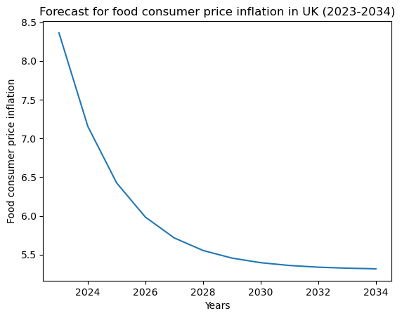
Based on this very simplistic model, one might conclude consumer food inflation is set to decrease steadily from 2023 onwards.
Footnotes
It is simplistic because it assumes stationarity of the modelled time series, which is an assumption that might not hold here!↩︎