✍️ Mini-Project 2 (30%): London Transport Journey Analysis

2025/26 Winter Term

🎯 Learning Goals

By the end of this assignment, you will: i) Design a defensible methodology for comparing journey times between Inner and Outer London, ii) Collect and store data from the TfL Journey Planner API, iii) Transform and merge API data with geographic context from the ONS Postcode Directory, iv) Communicate two insight-driven findings with visuals, v) Reflect on your analytical decisions, including AI support and source validation

This is your second graded summative assignment, worth 30% of your final mark. Mini-Project 2 builds directly on the workflow you developed for Mini-Project 1, but introduces a new API and a question that gives you more autonomy to choose your own direction.

⏳	Deadline	Wednesday, 1 April 2026 at 8 pm UK time
💎	Weight	30% of final grade
✋	GitHub Classroom	GitHub Classroom Repository (link on Moodle for registered students)

📌 Update announced on 19 March 2026: the deadline has been extended by one week so you have time to apply the EDA and visualisation techniques from 🖥️ W09 Lecture to your NB03 and REPORT.md.

📝 The Question

Just as you did in the ✍️ Mini Project 1, you are asked to investigate a specific question using predefined data sources.

This time, you are asked to investigate the question:

How does travelling between Inner London and Outer London change when it is done at peak versus off-peak hours?

This question is intentionally exploratory. You will have to decide what counts as Inner London, which part of Outer London to study, what peak and off-peak mean, and how to measure the difference. Your project must be scoped to answer this question given the requirements below.

GITHUB ASSIGNMENT INVITATION LINK:
https://classroom.github.com/a/H7YcSAlt

Click here for a 💡 TIP

💡 TIP ON HOW TO GET STARTED

Start simple. One Inner London origin, one Outer London destination. Make one peak request and one off-peak request. Get the data into a DataFrame. See if the difference matches your intuition. Git add, git commit, git push. Only then add more locations.

A single well-justified origin-destination pair with thorough analysis is a stronger submission than a dozen pairs with no clear reasoning.

📋 High-level requirements

Project structure

Your project MUST be structured as identified in the file tree below.

<your-github-repo-folder>/
├── notebooks/
│   ├── .env                                     # Not tracked by git
│   ├── NB01-Data-Collection.ipynb               # You create
│   ├── NB02-Data-Transformation.ipynb           # You create
│   └── NB03-Exploratory-Data-Analysis.ipynb     # You create
├── REPORT.md                                    # Two insights, narrative titles, visuals (or closeread alternative — see below)
├── README.md                                    # Project overview and reproduction notes
└── data/
    ├── raw/
    │   ├── london_postcodes-ons-postcodes-directory-feb22.csv         # Not tracked by git
    │   └── *.json                                                     # or *.csv files, your choice
    └── processed/
        └── *.csv

You will notice .gitkeep files inside some empty folders. Git does not track empty directories, so .gitkeep is a convention to make sure the folder structure survives when you clone the repo. You can safely ignore these files as they have no effect on your code. You can even delete them later if you want to.

Because your notebooks live inside notebooks/ but your data lives in data/, you will need to use ../data/raw/ and ../data/processed/ when reading or writing files from inside a notebook. The .env file sits next to your notebooks so load_dotenv() will find it automatically.

If you think you need to deviate from the above, ask in the #help Slack channel before the deadline.

Click here for a 💡 TIP

💡 TIP ABOUT THE FIRST COMMIT

Practice your Terminal and Git skills from the very start.

# If using Nuvolos, change to the correct directory first.
cd /files/<your-github-repo-folder>

# Create all necessary folders
mkdir -p data/raw data/processed

# Create remaining files
touch notebooks/.env
touch notebooks/NB01-Data-Collection.ipynb
touch notebooks/NB02-Data-Transformation.ipynb
touch notebooks/NB03-Exploratory-Data-Analysis.ipynb

git add notebooks/
git commit -m "Create empty notebooks"
git push

🗄️ Data sources

You MUST use data solely from these two specific data sources:

1. TfL API, more specifically the Journey Planner endpoint:

   https://api.tfl.gov.uk/Journey/JourneyResults/{from}/to/{to}

   Collect it using the requests library, as you have been doing in the course so far.

How to get a TfL API key

1. Go to api-portal.tfl.gov.uk and click on the ‘register’ link to sign up for an account. Use any e-mail address you like.

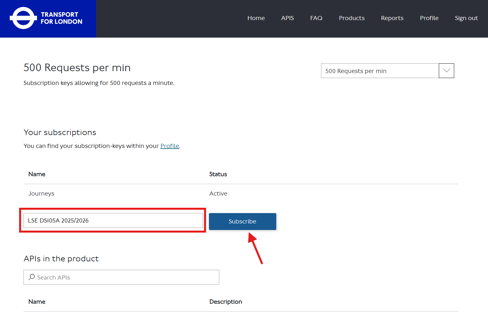
2. After signing in, go to the Products tab and find the ‘500 Requests per min’ product (or click 🔗 this direct link).

3. Subscribe to the product by entering some identifier in the textbox and clicking the ‘Subscribe’ button.

   

4. Click ‘Show’ to reveal your API key. Copy it and paste it into your notebooks/.env file:

   API_KEY=your_key_here

   You can always return to your TfL API - Profile page to check your key.

2. ONS Postcode Directory¹

   This is a static CSV you will download and load locally. It is in the .gitignore by default because of its size.

How to download the ONS Postcode Directory

1. Go to the ONS Postcode Directory page and click ‘Download’.

   Download the file called london_postcodes-ons-postcodes-directory-feb22.csv (122 MB) to your computer. DO NOT RENAME THIS FILE.

2. Upload it to the <your-github-repo-folder>/data/raw/ folder using the Nuvolos file explorer.

3. Confirm it is correctly gitignored:

   git status

   You should not see the CSV file listed. If it appears, something is wrong with your .gitignore.

Click here for a 💡 TIP about data collection

💡 TIP ON HOW TO GET STARTED

Start with just the from and to parameters. Use LSE’s postcode (WC2A 2AE) as your Inner London reference point, or justify a different choice. Pick one Outer London destination. Make one request. See what the JSON looks like. Make it tabular. Git add, git commit, git push. Only then expand.

📌 Your decisions and where to document them

📌 DECISIONS, DECISIONS, DECISIONS

You will need to make several decisions independently:

1. Inner London origin: Use LSE (WC2A 2AE) as your starting point, or justify any alternative Inner London location.

2. Outer London destination(s): Which specific postcode(s) will you use? You need at least one, but you may use more. How will you justify your choice? 📚 See Appendix for ONS columns that can help you select and contextualise your destinations.

3. Peak and off-peak definitions: What time window counts as peak? What counts as off-peak? How will you justify the distinction? (Hint: there may be official definitions you can reference.)

4. What you measure: Journey duration in minutes is the most natural metric, but the TfL API returns other fields too. Whatever you decide to measure, document it.

5. Anything else: Any other decision you make — modes of transport, specific API parameters, how you handled missing or thin responses — must be documented in REPORT.md.

Click here for 💡 TIPS

💡 TIPS ON HOW TO MAKE THE DECISIONS

1. Inner London origin: LSE is a reasonable default. If you choose something else, explain why in REPORT.md.

2. Outer London destinations: Start with one. Get data, explore it, then decide if more locations would strengthen your comparison.

3. Peak and off-peak: Read the TfL API documentation to understand the time and timeIs parameters. Do some research into how official bodies (TfL, the DfT) define peak hours for London. Document your source.

4. What you measure: Duration is a safe starting point. If you want to explore walking distance, number of transfers, or fare cost, that is fine — just justify the choice and be consistent.

🧰 Technical Requirements

1. You MUST add reflection notes in your notebooks to document your learning process.

   If you use AI in this assignment, share your chat logs in your notebooks or in your README.md. It helps us see your learning process directly.

What to write in the reflection notes

💭 **Personal Reflection Notes:**

* I tried to merge the TfL results with the ONS postcode data using [column X] but 
  got a KeyError. After checking the docs I realised [the issue]. The Claude bot 
  suggested [approach], which worked after I adjusted [Y].

2. All data collection MUST happen in notebooks/NB01 using the requests library.

Rate limiting guidance

Use time.sleep(2) between requests when looping over multiple postcodes:

for postcode in postcodes:
    response = requests.get(url, params=params)
    # process and save
    time.sleep(2)

3. Whatever data is produced in notebooks/NB01 MUST be saved to data/raw/ as JSON or CSV files.

4. You can use for loops in notebooks/NB01 for data collection, but you MUST use vectorised operations for analysis in notebooks/NB02 and notebooks/NB03.

   If you genuinely need a for loop in notebooks/NB02 or notebooks/NB03, document why a NumPy or pandas alternative would not work.

5. In notebooks/NB02, you MUST read from data/raw/ and save processed data to data/processed/ as CSV files.

6. In notebooks/NB03, you MUST read from data/processed/ and explore your data. Every plot you produce must use the plot_df pattern introduced in 🖥️ W05 Lecture and reinforced in 🖥️ W09 Lecture.

   🗒️ IMPORTANT: notebooks/NB03 is your research space. You can produce as many exploratory plots as you like. Only the two polished insights you select for REPORT.md will be marked. The rest can stay in notebooks/NB03 as evidence of exploration.

7. You MUST fill out the placeholders in README.md and REPORT.md, including whether and how you used AI tools.

What do you mean by ‘placeholders’?

In both the README and the REPORT, you will find square brackets with the text [TODO: ...]. Replace the entire bracketed section with your own text.

For example:

[TODO: explain _why_ you focused on the locations you chose].

becomes something like:

I selected Barking as my Outer London destination because its IMD rank suggested 
it might show a different pattern to Richmond, which I used for comparison.

✔️ How We Will Grade Your Work

Higher marks are reserved for those who demonstrate exceptional effort or insight in ways that align with the learning objectives and coding philosophy of this course. Adding more analysis or more locations without clear reasoning does not score higher.

Critical reminder: You are graded on your reasoning process and decision documentation. Correct output with weak justification scores lower than incorrect output with clear evidence of learning.

Coherence matters: We check whether your reflections match what your code actually does. If you use sophisticated techniques but cannot explain why, or cannot connect them to specific course activities, the marks will reflect that. Link decisions to specific activities: “I used .groupby().agg() as introduced in 🖥️ W07 Lecture” rather than “I used groupby.”

If you have engaged with the teaching materials and worked on the exercises, a Very Good! (70-75 marks) is achievable.

📥 Technical Implementation (0-30 marks)

Data collection, processing, and analysis quality

Marks awarded	Level	Description
<12 marks	Poor	Your code logic does not work (even if it runs). API authentication failed, wrong endpoint used, files are missing, credentials are hardcoded, or the code has too many errors to run.
12-14 marks	Weak	Your code runs but has multiple serious problems. Data collected does not help answer the question, loops used where vectorisation would work, credentials not secured, files disorganised, or code hard to follow.
15-17 marks	Fair	Your workflow works but has notable problems. API and collection function, but with concerning issues in organisation, data quality, or a disconnection between technique sophistication and what was taught.
18-20 marks	Good	Competent technical work. API working, vectorised operations used, credentials secured, files organised. Techniques beyond the course are accompanied by some explanation of why they were appropriate.
21-23 marks	Very Good!	Clean technical execution with data validation and security. No hardcoded keys. Data quality issues acknowledged and handled where present. Vectorised operations used effectively. Code sophistication matches written explanations.
24+ marks	🏆 WOW	Exceptional technical implementation. Exceptionally clean pandas transformations, professional function design, exemplary organisation, sophisticated data quality checks. Nothing is over-engineered: every choice serves a clear purpose.

📊 Communication & Insights (0-40 marks)

Your insights, exploration process, and reflections

Marks awarded	Level	Description
<16 marks	Poor	Your analysis does not answer the question or has fundamental problems. Insights missing, seaborn not used, axes unlabelled or misleading, interpretation wrong or absent, no awareness of statistical reasoning.
16-19 marks	Weak	You attempted analysis but it does not work well. Visualisations do not support the claims, titles describe the chart rather than state a finding, shallow interpretation, inappropriate statistical choices without justification.
20-23 marks	Fair	Your analysis produces some insights but has notable weaknesses. Analytical work present, but significant weaknesses in communication, statistical reasoning, or disconnection between technique and course content.
24-27 marks	Good	Competent analysis with reasonable insights. Two insights with acceptable visualisations, reasonable interpretation, appropriate statistical choices with some justification, vectorised operations used.
28-31 marks	Very Good!	Two compelling insights with narrative titles. Statistical choices (mean vs median) justified. Visualisations correctly interpreted. Correlation vs causation acknowledged. notebooks/NB03 exploration shows genuine analytical thinking. Reflections connect to course activities.
32+ marks	🏆 WOW	Exceptional analysis with compelling narrative. Publication-quality visualisations, sophisticated seaborn styling, nuanced pattern discovery, convincing narrative, sophisticated statistical reasoning throughout.

🧐 Research & Methodology Design (0-30 marks)

How you defined and justified your approach

Marks awarded	Level	Description
<12 marks	Poor	Key methodology documentation is missing or critically flawed. No clear Inner or Outer London definition, peak and off-peak not specified, or the approach is so unclear we cannot assess it.
12-14 marks	Weak	Methodology submitted but multiple serious problems. Definitions vague or unexplained, decisions not justified, location selection arbitrary, or several key elements missing.
15-17 marks	Fair	Adequate methodology with notable weaknesses. Approach defined but justifications are generic, decision-making process unclear, or little connection to course content.
18-20 marks	Good	Competent methodology with reasonable justification. Clear definitions of Inner and Outer London, peak and off-peak justified, location selection explained. Some connection to course materials.
21-23 marks	Very Good!	Thoughtful methodology with clear reasoning. All key decisions are specific and justified. Written methodology matches implementation. Evidence of genuine analytical thinking rather than surface completion. ONS data incorporated in a way that strengthens the methodology or the analysis.
24+ marks	🏆 WOW	Exceptional methodology with sophisticated understanding. Publishable-quality methodological design, deep justification drawing on external sources, creative and defensible use of ONS data to contextualise or extend the analysis.

♟️ A Tactical Plan (W07-W09)

Week	Focus	Key Tasks
W07	Setup & first collection	Accept the assignment and clone the repository into Nuvolos. Set up the repo structure. Get the TfL API key working. Make at least one peak and one off-peak request for your chosen route. Save raw JSON to data/raw/. Document your initial decisions in REPORT.md before you forget.
W08	Transformation & merging	Use the ONS Postcode Directory to contextualise your postcode selection. Build notebooks/NB02: load from data/raw/, merge API data with ONS attributes, apply vectorised transformations, save to data/processed/. Document any new decisions in REPORT.md.
W09	Exploration & communication	Build notebooks/NB03: explore your data freely, produce many plots, identify the two most compelling findings. Polish those two insights with narrative titles and clean visualisations. Draft REPORT.md (or closeread alternative). Check everything runs from a clean state.
W10	Submission	Deadline is Monday 8 pm. Review README.md and REPORT.md are complete. Push a final commit.

🚀 If you want to go the extra mile

If you are aiming for a distinction and have the time, here are some directions worth exploring:

• Richer temporal comparison: Test the same route across multiple time windows (weekday morning peak, weekday evening peak, weekend midday). This can reveal patterns that a single peak/off-peak comparison misses.

• ONS socioeconomic context: Use the imd column to explore whether Outer London destinations with higher deprivation scores show different peak/off-peak patterns. Read the IMD caveats in the Appendix first. 📚 See Appendix

• LSOA-level aggregation: Instead of individual postcodes, sample multiple postcodes within an LSOA and aggregate journey metrics by area. This gives you a more robust comparison at the neighbourhood level. 📚 See Appendix

• Closeread presentation: Replace your REPORT.md with a scrollytelling narrative built with closeread. See below for details.

These extensions require more API calls, careful rate limiting, and more sophisticated analysis. Start with the baseline approach first.

📰 Optional: Replace REPORT.md with a Closeread Narrative

Closeread is a Quarto extension that lets you build scrollytelling documents where text narrates alongside highlighted or zoomed visuals. If you use it well, it can make your two insights far more compelling than a plain markdown file.

This is entirely optional and is one route to WOW-level Communication & Insights marks. It fully replaces REPORT.md: you do not need to submit both.

🗒️ Note: If you go the closeread route, because you will be telling a story, you can do more than just 2 insights. I won’t set an upper limit but be careful not to overcomplicate or to add too many things that would detract from the story.

You will get an introduction to closeread in 🖥️ W09 Lecture.

📮 Need Help?

• Post questions in the #help Slack channel.
• Check the ✋ Contact Hours page for support times.
• Book office hours via StudentHub for more detailed conversations.

Start with the simple approach. Keep your reflections purposeful. Give yourself time before the deadline to polish the two insights you are most proud of.

---

📚 Appendix: ONS Postcode Directory Data Dictionary

Most Important Columns

Column	Type	Description	Example	Your Use
pcds	string	Postcode with space	SW1A 2AA	TfL API input, human-readable
lsoa11	string	Lower Super Output Area (2011 Census)	E01004736	Neighbourhood unit (~1,500 people) for aggregation
oslaua	string	Local Authority code (Borough)	E09000033	Borough context (Westminster = E09000033)
lat	float	Latitude (WGS84 decimal degrees)	51.5074	Straight-line distance calculations
long	float	Longitude (WGS84 decimal degrees)	-0.1278	Paired with latitude for distance calculations

Data source: London Datastore - ONS Postcode Directory

Geographic Hierarchy (How Areas Nest)

Individual Postcode (your API query unit)
    ↓ ~400 postcodes aggregate into
Output Area (OA11) - ~300 residents
    ↓ ~5 OAs aggregate into
Lower Super Output Area (LSOA11) - ~1,500 residents ← USEFUL FOR AGGREGATION
    ↓ ~5 LSOAs aggregate into
Middle Super Output Area (MSOA11) - ~7,500 residents
    ↓ Multiple MSOAs per
Borough (oslaua) - ~300,000 residents (33 London boroughs)

Tactical approach: Use individual postcodes, note their LSOA for context.

Ambitious approach: Sample postcodes within LSOAs, aggregate journey metrics by LSOA to compare neighbourhood-level patterns.

Full technical guide: ONS Postcode Products Documentation

Critical Data Handling Notes

Filter to current postcodes only:

df_active = df[df['doterm'].isna()].copy()

Postcode format for TfL API:

Both SW1A 2AA (with space) and SW1A2AA (without) should work. You can use the pcds column directly.

London borough codes:

All start with E09, ranging from E09000001 (City of London) to E09000033 (Westminster).

Additional Columns (for ambitious students)

Column	Type	Description	Range/Format	When to Use
imd	integer	Index of Multiple Deprivation rank for the LSOA	1 (most deprived) to 32,844 (least deprived)	Explore whether deprived areas show different peak/off-peak patterns. ⚠️ This value is the same for all postcodes within the same LSOA.
usertype	integer	Postcode classification	0 = residential, 1 = business	Filter to residential postcodes if analysing where people live
osward	string	Electoral Ward code	Alphanumeric	Sub-borough analysis
ttwa	string	Travel To Work Area code	Alphanumeric	Useful to validate whether your locations reflect actual commute patterns
oac11	string	Output Area Classification	Alphanumeric codes	Neighbourhood type classification (e.g., ‘cosmopolitan students’). Requires research to use correctly.

Reference Codes (research required if using)

Column	Full Name	What You’d Need to Research
dointr	Date of introduction	YYYYMM format, postcode lifecycle
doterm	Date of termination	YYYYMM or NULL, active vs terminated
oseast1m	OS Grid Easting	British National Grid coordinate system
osnrth1m	OS Grid Northing	Alternative to lat/long, needs conversion
pcon	Parliamentary Constituency	Westminster MP constituencies
bua11	Built-Up Area 2011	Continuous urban settlement definition
wz11	Workplace Zone 2011	Areas with 200-625 workers
pfa	Police Force Area	Policing jurisdiction

⚠️ These require research. If you want to use any of these columns, spend time on the ONS Geography Portal understanding what they represent. Most are unnecessary for answering the core question.

Footnotes

1. A more recent version of the ONS Postcode Directory (May 2024) is available from the ONS Open Geography Portal, but it contains UK-wide postcodes which is too much data for this assignment. We use the London-specific February 2022 version to keep the dataset manageable.

   📚 See the Appendix: ONS Postcode Directory Data Dictionary for essential columns, geographic hierarchy, and data handling notes.