🗓️ Week 07:
Unsupervised Learning
Clustering
11/11/22
Recall the Supervised Learning approach
Example of Supervised Models
From 🗓️ Week 02:
The generic supervised model:
\[ Y = \operatorname{f}(X) + \epsilon \]
is defined more explicitly according to each algorithm ➡️
Multiple Linear Regression
\[ \begin{align} Y = \beta_0 &+ \beta_1 X_1 + \beta_2 X_2 \\ &+ \dots \\ &+ \beta_p X_p + \epsilon \end{align} \]
when there are multiple predictors, \(X_p\).
Multiple Logistic Regression
\[ \begin{align} Y \propto p(X) &= \\ &= \frac{e^{\beta_0 + \beta_1 X_1 + \ldots + \beta_p X_p}}{1 + e^{\beta_0 + \beta_1 X_1 + \ldots + \beta_p X_p}} \end{align} \]
when there are multiple predictors, \(X_p\).
Unsupervised Learning
How is it different?
Supervised Learning
- Our main goal is to predict future values of \(Y\)
- We have historic \(X\) and \(Y\) data
- Algorithms fit the data and supervise themselves objectively (e.g.: residuals)
- We can validate how well the model fits training data and how it generalises beyond that.
Unsupervised Learning
- The main goal is to observe (dis-)similarities in \(X\)
- We only have \(X\) data
- There is no \(Y\) variable to “supervise” how models should fit the data
- Validation is a lot more subjective. There is no objective way to check our work.
Clustering
Why clustering?
- Are there clusters (subgroups) in my data?
- Which samples are most similar to each other?
- Are there samples that do not fall in any subgroup?
Each algorithm is different
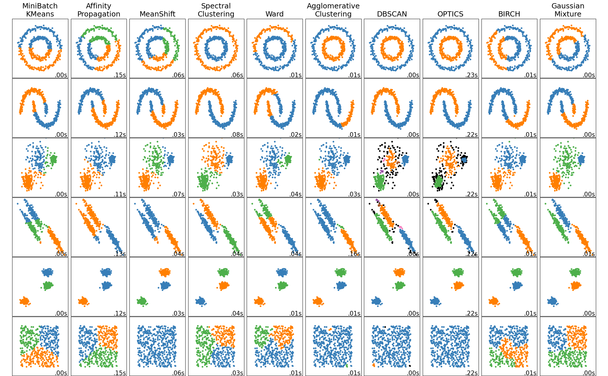
An Example:
- Let’s use the 🐧 penguins data to illustrate clustering
- Same data used in 💻 Week 07 - Lab
🐧 penguins data
Code
# A tibble: 15 × 5
   species bill_length_mm bill_depth_mm flipper_length_mm body_mass_g
   <fct>            <dbl>         <dbl>             <int>       <int>
 1 Adelie            39.1          18.7               181        3750
 2 Adelie            39.5          17.4               186        3800
 3 Adelie            40.3          18                 195        3250
 4 Adelie            36.7          19.3               193        3450
 5 Adelie            39.3          20.6               190        3650
 6 Adelie            38.9          17.8               181        3625
 7 Adelie            39.2          19.6               195        4675
 8 Adelie            41.1          17.6               182        3200
 9 Adelie            38.6          21.2               191        3800
10 Adelie            34.6          21.1               198        4400
11 Adelie            36.6          17.8               185        3700
12 Adelie            38.7          19                 195        3450
13 Adelie            42.5          20.7               197        4500
14 Adelie            34.4          18.4               184        3325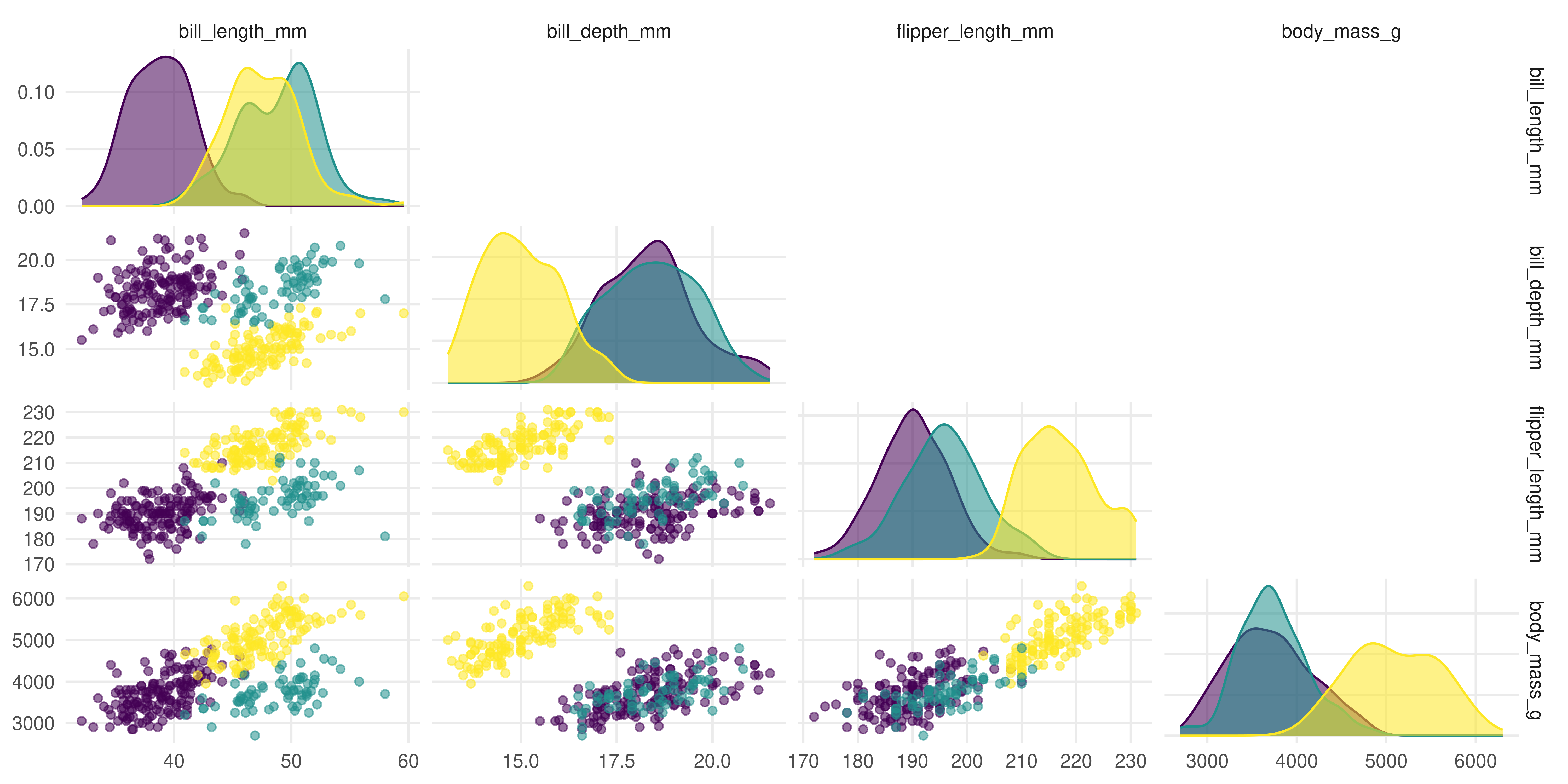
15 Adelie 46 21.5 194 4200Correlation plot
It is easy to distinguish the species using colour because we have a species column:
Source Code
Tip
- Use the code below to replicate the plot from the previous slide.
- Found a bug? Report it on Slack.
library(GGally)         # pretty correlation plots
library(tidyverse)      # to use things like the pipe (%>%), mutate and if_else
library(palmerpenguins) # for penguin data

penguins_cleaned <-
  penguins %>%
  na.omit() %>%
  select(species, where(is.numeric), - year)

# View(penguins_cleaned) or do head(penguins_cleaned)

g <-
  ggpairs(penguins_cleaned,
        aes(colour = species, fill = species, alpha = 0.875),
        columns = 2:5,
        upper = list(continuous = 'blankDiag')) +
  theme_minimal() +
  theme(panel.grid.minor = element_blank()) +
  scale_colour_viridis_d() +
  scale_fill_viridis_d() +
  labs(colour = 'Species', fill = 'Species')

g
Penguins data without the species
What if we did not have the species column?
# A tibble: 15 × 4
   bill_length_mm bill_depth_mm flipper_length_mm body_mass_g
            <dbl>         <dbl>             <int>       <int>
 1           39.1          18.7               181        3750
 2           39.5          17.4               186        3800
 3           40.3          18                 195        3250
 4           36.7          19.3               193        3450
 5           39.3          20.6               190        3650
 6           38.9          17.8               181        3625
 7           39.2          19.6               195        4675
 8           41.1          17.6               182        3200
 9           38.6          21.2               191        3800
10           34.6          21.1               198        4400
11           36.6          17.8               185        3700
12           38.7          19                 195        3450
13           42.5          20.7               197        4500
14           34.4          18.4               184        3325
15           46            21.5               194        4200
K-Means Clustering
Objective function:
Find a partition \(C_1 \cup C_2 \cup C_3 \cup \ldots \cup C_K = \{1, \ldots, n\}\) for the data such that: \[ \text{minimize}_{C_1, \ldots, C_K} \left\{ \sum_{k=1}^{K}{\frac{1}{|C_k|} \sum_{i,i' \in C_k}{\sum_{j=1}^p{(x_{ij} - x_{i'j})^2}} }\right\} \]
K-Means algorithm
Step by step of one clustering algorithm:
- You have to inform \(K\), the number of clusters you wish to recover
- The algorithm randomly assign each observation to a random cluster
- Iterate until cluster assignments stop changing
- For each of the \(K\) clusters, compute the cluster centroid
- Re-assign samples to their closest centroid (euclidean distance)
Clustering Penguins
K-means clustering with 3 clusters of sizes 113, 80, 140

Cluster means:
  bill_length_mm bill_depth_mm flipper_length_mm body_mass_g
1       44.24336      17.44779          201.5487    4310.619
2       48.66250      15.39750          219.9875    5365.938
3       41.12214      17.94643          189.6286    3461.250

Clustering vector:
  [1] 3 3 3 3 3 3 1 3 3 1 3 3 1 3 1 3 3 3 1 3 3 3 3 3 1 3 1 3 1 3 1 1 3 3 1 3 1
 [38] 3 1 3 1 3 3 1 3 1 3 1 3 3 3 3 3 3 3 1 3 1 3 1 3 1 3 1 3 1 3 1 3 1 3 1 3 1
 [75] 3 1 3 1 3 3 3 3 1 3 3 1 3 1 3 1 3 1 3 1 3 1 3 1 3 3 3 1 3 1 3 1 3 1 1 1 3
[112] 3 3 3 3 3 3 3 3 1 3 1 3 1 3 3 3 1 3 1 3 1 3 1 3 3 3 3 3 3 1 3 3 3 3 1 1 2
[149] 1 2 2 1 1 2 1 2 1 2 1 2 1 2 1 2 1 2 2 2 1 2 2 2 2 1 2 2 1 2 2 2 2 2 2 1 2
[186] 1 2 1 1 2 2 1 2 2 2 2 2 1 2 2 2 1 2 1 2 1 2 1 2 1 2 2 1 2 1 2 2 2 1 2 1 2
[223] 1 2 1 2 1 2 1 2 1 2 2 2 2 2 1 2 2 2 2 2 1 2 2 2 2 2 2 1 2 1 2 2 2 1 2 1 2
[260] 2 2 2 2 2 2 3 1 3 3 3 1 3 3 1 3 3 3 3 1 3 1 3 3 3 1 3 3 3 3 3 1 3 3 3 1 3
[297] 1 3 1 3 1 3 1 3 1 1 3 3 3 3 1 3 1 3 3 3 1 3 1 3 3 3 1 3 3 1 3 3 1 3 3 1 3

Within cluster sum of squares by cluster:
[1] 9318036 9718829 9724809
 (between_SS / total_SS =  86.6 %)

Available components:

[1] "cluster"      "centers"      "totss"        "withinss"     "tot.withinss"
[6] "betweenss"    "size"         "iter"         "ifault"
Inspect the centroids
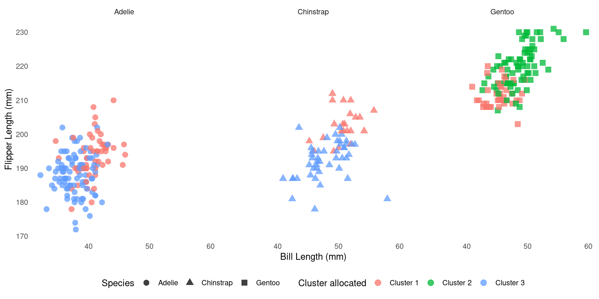
How does it compare to the real one?
We can cross-tabulate species and cluster membership:
Visual comparison
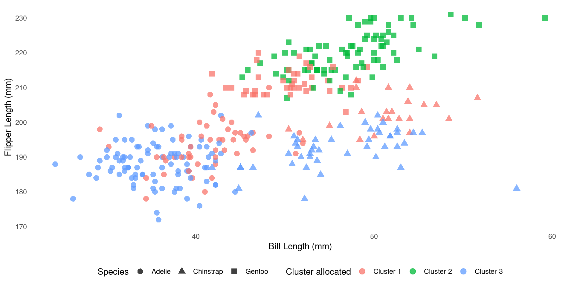
Visual comparison
What’s Next
- Next week, Week 08, the labs will be about SVM & cross-validation
- Revisit 🗓️ Week 05 lecture
- Read “The cross-validation setup” section in Week 04 page
- You will explore k-means clustering in Week 09 labs
References

DS202 - Data Science for Social Scientists 🤖 🤹