
🗓️ Week 02:
Linear Regression
DS202 Data Science for Social Scientists
10/7/22
Linear Regression with a single predictor
We want to estimate:
\[ \hat{y} = \hat{\beta_0} + \hat{\beta_1} x \]
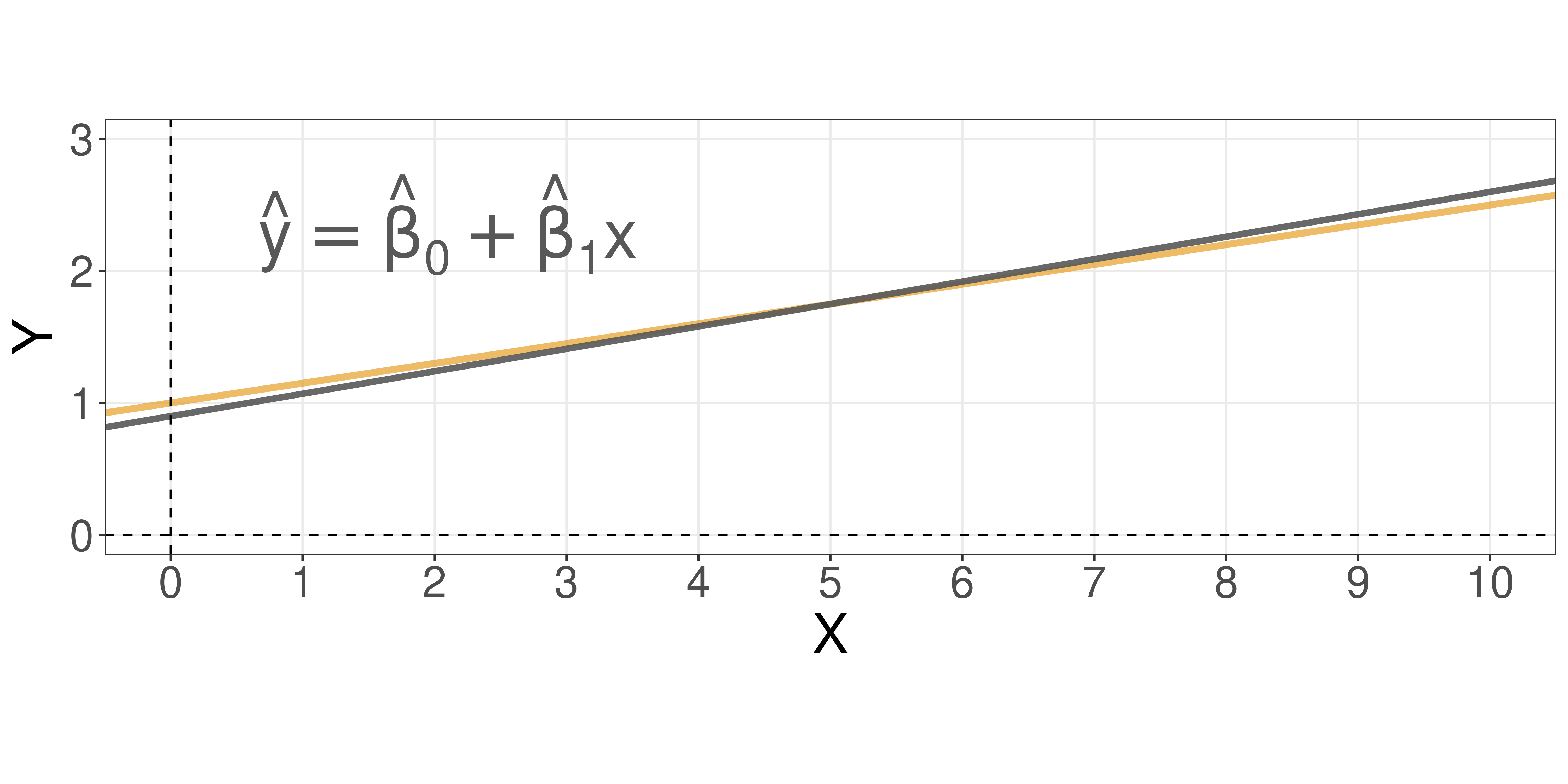
where:
- \(\hat{y}\): is a prediction of \(Y\) on the basis of \(X = x\).
- \(\hat{\beta_0}\): is an estimate of the “true” \(\beta_0\).
- \(\hat{\beta_1}\): is an estimate of the “true” \(\beta_1\).
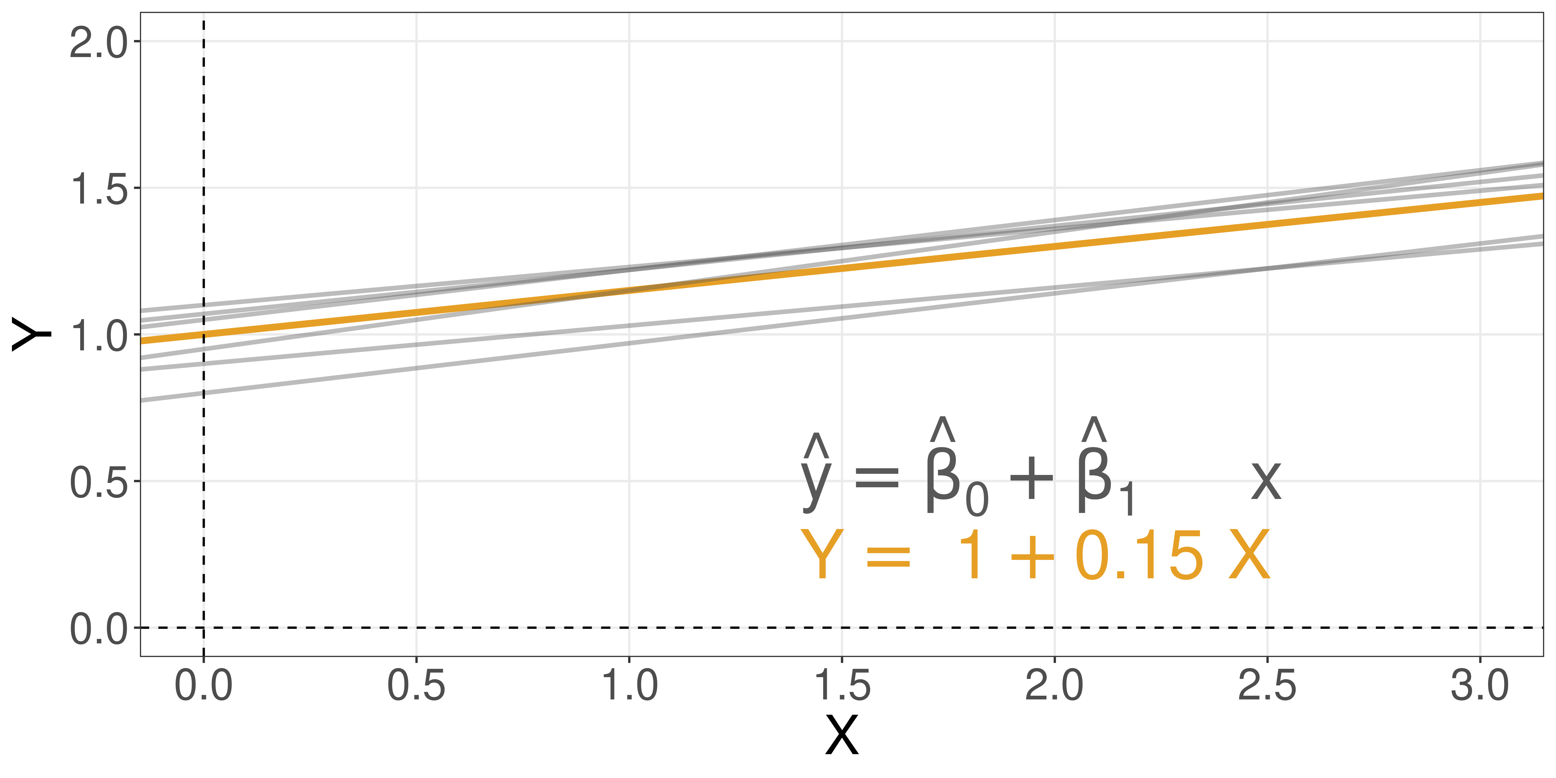
Different estimators, different equations
There are multiple ways to estimate the coefficients.
- If you use different techniques, you might get different equations
- The most common algorithm is called
Ordinary Least Squares (OLS) - Just to name a few other estimators (Karafiath 2009):
- Least Absolute Deviation (LAD)
- Weighted Least Squares (WLS)
- Generalized Least Squares (GLS)
- Heteroskedastic-Consistent (HC) variants
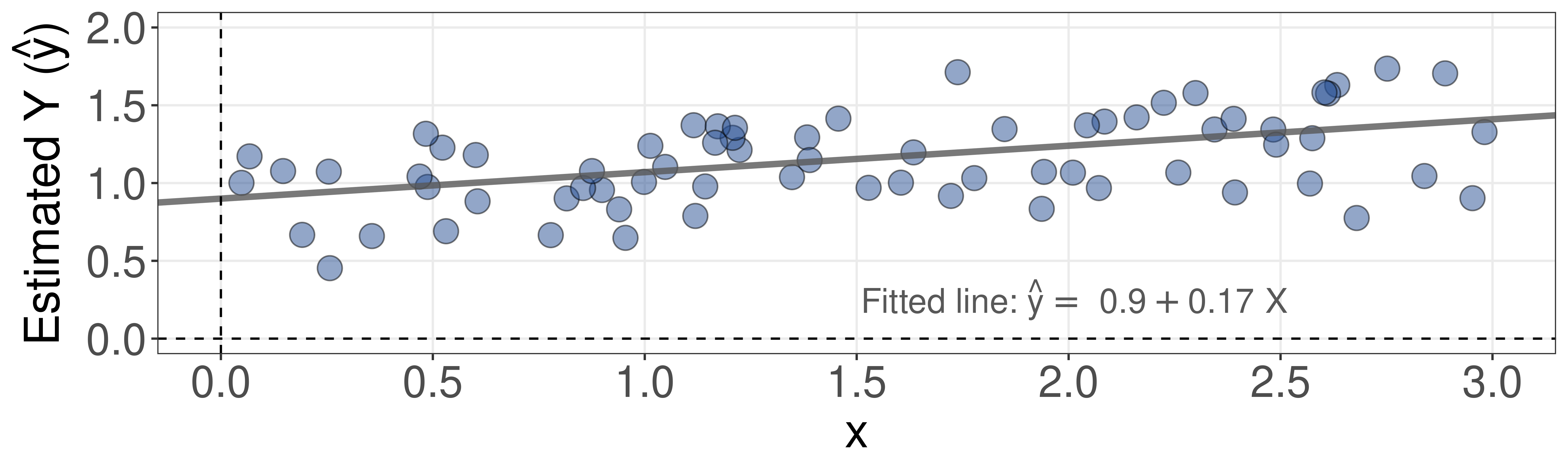
The concept of residuals
Suppose you came across some data:

The concept of residuals
So, you decide to fit a line to it.
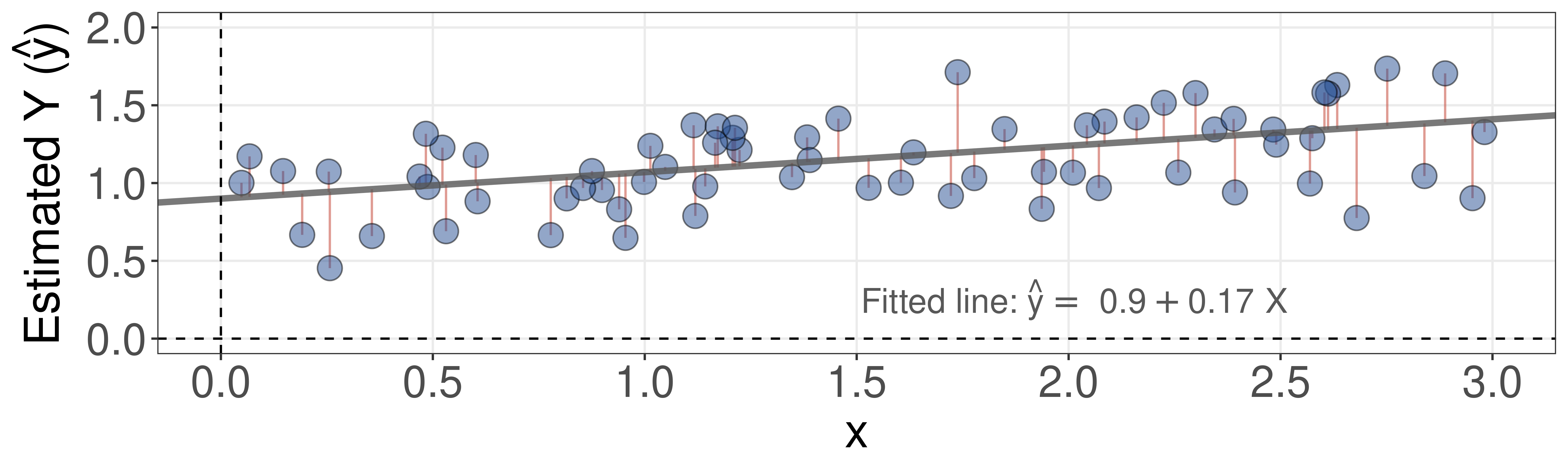
The concept of residuals
Residuals are the distances from each data point to this line.
A question for you

Why the squares and not, say, just the sum of residuals?
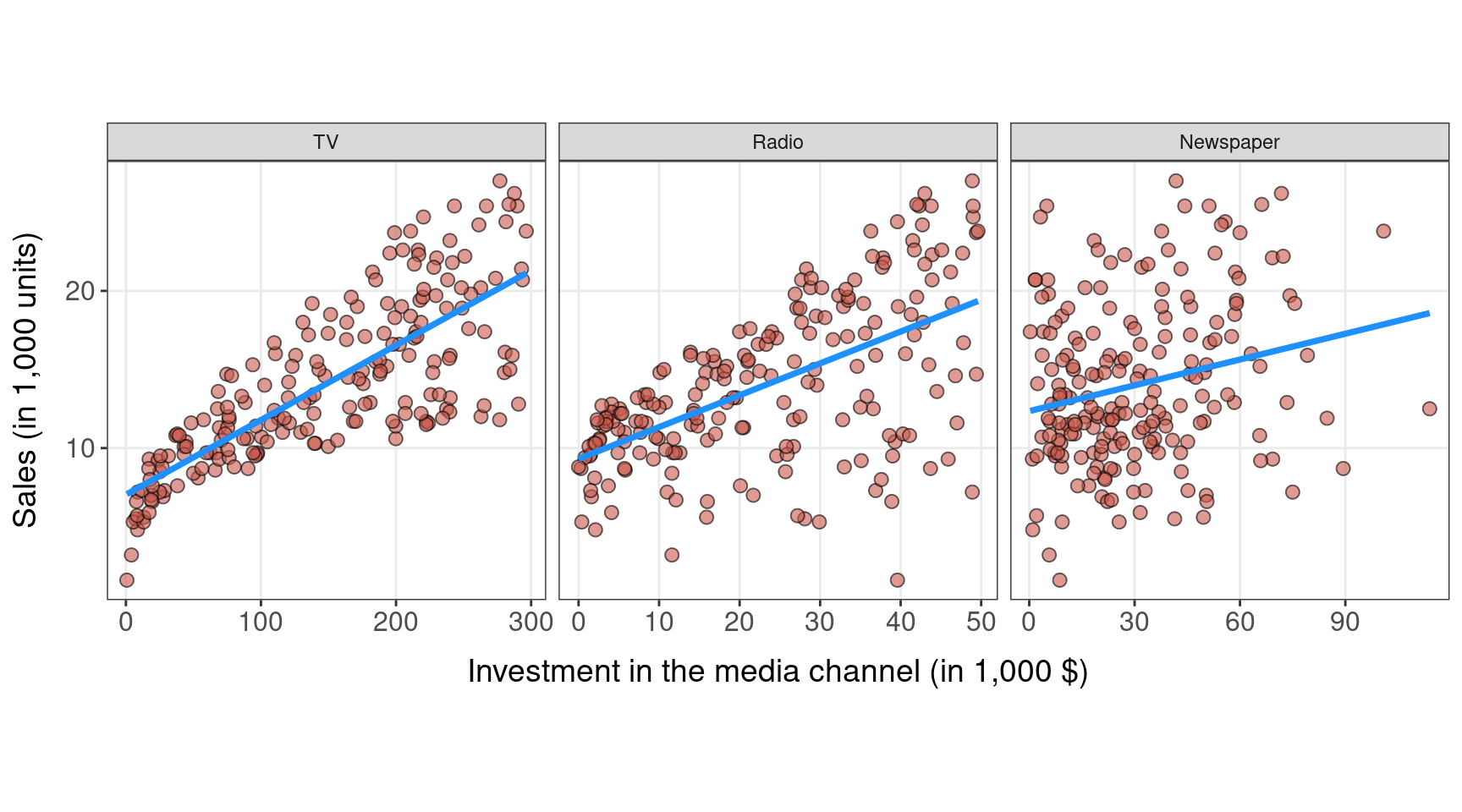
Relationship: advertising budget and sales
Is advertising spending related to sales?
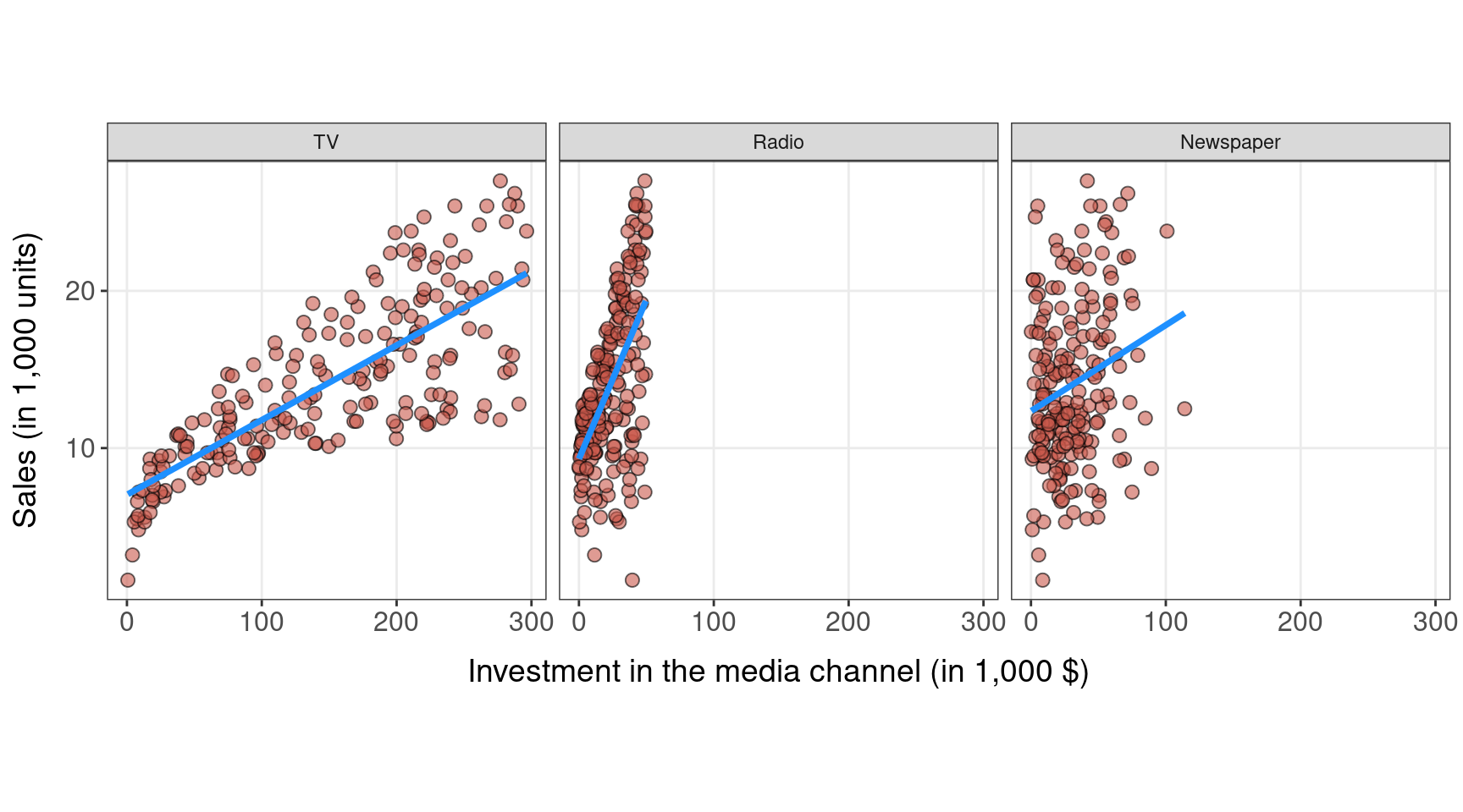
Relationship: advertising budget and sales
Is advertising spending related to sales?
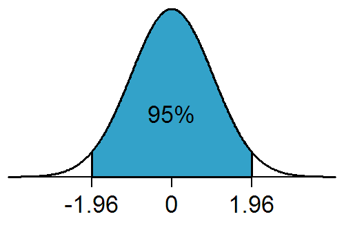
Confidence Intervals
- If we were to fit a linear model from repeated samples of the data, we would get different coefficients every time.
- Because of the Central Limit Theorem, we know that the mean of this sampling distribution can be approximated by a Normal Distribution.
- We know from Normal Theory that 95% of the distribution lies within two times the standard deviation (centered around the mean).
A 95% confidence interval is defined as a range of values such that with 95% probability, the range will contain the true unknown value of the parameter.
References
Altman, Douglas G, and J Martin Bland. 2005. “Standard Deviations and Standard Errors.” BMJ 331 (7521): 903. https://doi.org/10.1136/bmj.331.7521.903.
James, Gareth, Daniela Witten, Trevor Hastie, and Robert Tibshirani. 2021. An Introduction to Statistical Learning: With Applications in R. Second edition. Springer Texts in Statistics. New York NY: Springer. https://www.statlearning.com/.
Karafiath, Imre. 2009. “Is There a Viable Alternative to Ordinary Least Squares Regression When Security Abnormal Returns Are the Dependent Variable?” Review of Quantitative Finance and Accounting 32 (1): 17–31. https://doi.org/10.1007/s11156-007-0079-y.
