import numpy as np
import pandas as pd
from plotnine import *DS101 Lab 2: Importing and exporting structured data to and from Python
Below is the script that was showcased during the week 2 class. You can try it for yourselves on Google Colab.
Click on the button below to download the source file (.ipynb notebook) as well as data file (.csv) that were used to create this page, if you ever want to try the demo for yourselves:
Tracking socio-economic outcomes in the BRICS
Working with Python using Jupyter notebooks
Jupyter notebooks are a useful scratchpad for working with data.
The notebook structure means code is entered and prcessed inside individual cells, rather than as entire (end-to-end) script. Jupyter works with Python, and Google Colab is a cloud store for Jupyter notebooks attached to a backend that can run your code – without having to worry about the details of installing many packages (and their dependencies).
- Place the cursor inside a cell to make edits
- Press
shift+ENTER to run the code in a cell - That progresses the cursor to the next cell
Just follow the instructions above each cell. Ask for help with any technical problems.
Outline
We undertake the following steps:
- Source information
- Gather data
- Storage
- Load
- Clean
- Pre-process
- Build a dataset
- EDA
- Processing
- Visualisation
- Export
Getting started with Python
Loading libraries
Powerful languages like Python and R thrive on the ecosystem of user-created packages.
We import (or, “load”) a few of these packages here:
numpy– gives python more efficient way to work with arrayspandas– gives a way to work with (row and column) labelled arrays
These are very common modules to use whenever you want to work with datasets.
Sourcing data
On the left-handside, create a new folder DS101A_data and drop your WDI_metrics.csv file here
Loading data
Loading data into Python is fairly straightforward. We use a file path which tells Python where to look for the data followed by a / separator followed by the name of the file (WDI_metrics.csv).
Python provides the os module (Operating System Interface) – with dozens of functions for interacting with the operating system: https://docs.python.org/3/tutorial/stdlib.html
It’s a part of the standard library (i.e. the core of Python), and it mirrors the way that you would work with your own operating system if your were doing that by hand (or from the command line).
“cwd” means “current working directory”
To find out what your working directory is, we can import the os module and use the function: os.getcwd().
import os
os.getcwd()'/home/runner/work/DS101/DS101/2024/autumn-term/weeks/week02'We are going to load our data into a python module called pandas – it is specialised for handling tables of data called “dataframes”
- In this case, our variable is called
wb_metrics, and that hold our dataframe
wb_metrics = pd.read_csv("DS101A_data/WDI_metrics.csv", na_values="..").dropna(subset = "Series Code")Dataset exploration
What does this data look like?
Just “print” the dataframe
- Replace this code with
wb_metrics.head() - Try using different integers inside the brackets:
- e.g.
wb_metrics.head(1)
wb_metrics.head(3)| Series Name | Series Code | Country Name | Country Code | 2000 [YR2000] | 2001 [YR2001] | 2002 [YR2002] | 2003 [YR2003] | 2004 [YR2004] | 2005 [YR2005] | 2006 [YR2006] | 2007 [YR2007] | 2008 [YR2008] | 2009 [YR2009] | 2010 [YR2010] | 2011 [YR2011] | 2012 [YR2012] | 2013 [YR2013] | 2014 [YR2014] | 2015 [YR2015] | |
|---|---|---|---|---|---|---|---|---|---|---|---|---|---|---|---|---|---|---|---|---|
| 0 | Population, total | SP.POP.TOTL | Afghanistan | AFG | 19542982.0 | 19688632.0 | 21000256.0 | 22645130.0 | 23553551.0 | 24411191.0 | 25442944.0 | 25903301.0 | 26427199.0 | 27385307.0 | 28189672.0 | 29249157.0 | 30466479.0 | 31541209.0 | 32716210.0 | 33753499.0 |
| 1 | Population, total | SP.POP.TOTL | Albania | ALB | 3089027.0 | 3060173.0 | 3051010.0 | 3039616.0 | 3026939.0 | 3011487.0 | 2992547.0 | 2970017.0 | 2947314.0 | 2927519.0 | 2913021.0 | 2905195.0 | 2900401.0 | 2895092.0 | 2889104.0 | 2880703.0 |
| 2 | Population, total | SP.POP.TOTL | Algeria | DZA | 30774621.0 | 31200985.0 | 31624696.0 | 32055883.0 | 32510186.0 | 32956690.0 | 33435080.0 | 33983827.0 | 34569592.0 | 35196037.0 | 35856344.0 | 36543541.0 | 37260563.0 | 38000626.0 | 38760168.0 | 39543154.0 |
Pandas allows us to view different portion of our dataframe, using e.g. .iloc[]:
- The first integer is the row
- The second integer is the column
We can specify rows an columns using named labels too.
Here we select column subsets using the “slice” notation – try changing the values
wb_metrics.iloc[0:4, 0:10]| Series Name | Series Code | Country Name | Country Code | 2000 [YR2000] | 2001 [YR2001] | 2002 [YR2002] | 2003 [YR2003] | 2004 [YR2004] | 2005 [YR2005] | |
|---|---|---|---|---|---|---|---|---|---|---|
| 0 | Population, total | SP.POP.TOTL | Afghanistan | AFG | 19542982.0 | 19688632.0 | 21000256.0 | 22645130.0 | 23553551.0 | 24411191.0 |
| 1 | Population, total | SP.POP.TOTL | Albania | ALB | 3089027.0 | 3060173.0 | 3051010.0 | 3039616.0 | 3026939.0 | 3011487.0 |
| 2 | Population, total | SP.POP.TOTL | Algeria | DZA | 30774621.0 | 31200985.0 | 31624696.0 | 32055883.0 | 32510186.0 | 32956690.0 |
| 3 | Population, total | SP.POP.TOTL | American Samoa | ASM | 58230.0 | 58324.0 | 58177.0 | 57941.0 | 57626.0 | 57254.0 |
wb_metrics.shape(11067, 20)wb_metrics.columnsIndex(['Series Name', 'Series Code', 'Country Name', 'Country Code',
'2000 [YR2000]', '2001 [YR2001]', '2002 [YR2002]', '2003 [YR2003]',
'2004 [YR2004]', '2005 [YR2005]', '2006 [YR2006]', '2007 [YR2007]',
'2008 [YR2008]', '2009 [YR2009]', '2010 [YR2010]', '2011 [YR2011]',
'2012 [YR2012]', '2013 [YR2013]', '2014 [YR2014]', '2015 [YR2015]'],
dtype='object')wb_metrics.info()<class 'pandas.core.frame.DataFrame'>
Index: 11067 entries, 0 to 11066
Data columns (total 20 columns):
# Column Non-Null Count Dtype
--- ------ -------------- -----
0 Series Name 11067 non-null object
1 Series Code 11067 non-null object
2 Country Name 11067 non-null object
3 Country Code 11067 non-null object
4 2000 [YR2000] 7943 non-null float64
5 2001 [YR2001] 7816 non-null float64
6 2002 [YR2002] 7915 non-null float64
7 2003 [YR2003] 8084 non-null float64
8 2004 [YR2004] 8214 non-null float64
9 2005 [YR2005] 8324 non-null float64
10 2006 [YR2006] 8376 non-null float64
11 2007 [YR2007] 8432 non-null float64
12 2008 [YR2008] 8455 non-null float64
13 2009 [YR2009] 8524 non-null float64
14 2010 [YR2010] 8597 non-null float64
15 2011 [YR2011] 8630 non-null float64
16 2012 [YR2012] 8646 non-null float64
17 2013 [YR2013] 8633 non-null float64
18 2014 [YR2014] 8725 non-null float64
19 2015 [YR2015] 8443 non-null float64
dtypes: float64(16), object(4)
memory usage: 1.8+ MBReadability
The column labels are not great, in particular, they contain square brackets [ and ] which could easily be mistaken for (what are known as) operators within python: python thinks a symbol like this means you are working with “lists”
Let’s get rid of these and make our code more readable for human beings in the process
colnames = ["series_name", "series_code", "country_name", "country_code"]
colnames = colnames + ["yr_" + str(x) for x in range(2000, 2016)]
wb_metrics.columns = colnames
Column names
print(wb_metrics.columns)Index(['series_name', 'series_code', 'country_name', 'country_code', 'yr_2000',
'yr_2001', 'yr_2002', 'yr_2003', 'yr_2004', 'yr_2005', 'yr_2006',
'yr_2007', 'yr_2008', 'yr_2009', 'yr_2010', 'yr_2011', 'yr_2012',
'yr_2013', 'yr_2014', 'yr_2015'],
dtype='object')Fix to reflect the categorical nature of the datatype
In the “series name”, “series code” and “country code” columns. We will stick with strings for “country name” for now
wb_metrics_cat = wb_metrics.copy()
wb_metrics_cat[["series_name", "series_code", "country_code"]] = wb_metrics_cat[["series_name", "series_code", "country_code"]].astype("category")
wb_metrics_cat[["country_name"]] = wb_metrics_cat[["country_name"]].astype("string")
wb_metrics_cat.info()
<class 'pandas.core.frame.DataFrame'>
Index: 11067 entries, 0 to 11066
Data columns (total 20 columns):
# Column Non-Null Count Dtype
--- ------ -------------- -----
0 series_name 11067 non-null category
1 series_code 11067 non-null category
2 country_name 11067 non-null string
3 country_code 11067 non-null category
4 yr_2000 7943 non-null float64
5 yr_2001 7816 non-null float64
6 yr_2002 7915 non-null float64
7 yr_2003 8084 non-null float64
8 yr_2004 8214 non-null float64
9 yr_2005 8324 non-null float64
10 yr_2006 8376 non-null float64
11 yr_2007 8432 non-null float64
12 yr_2008 8455 non-null float64
13 yr_2009 8524 non-null float64
14 yr_2010 8597 non-null float64
15 yr_2011 8630 non-null float64
16 yr_2012 8646 non-null float64
17 yr_2013 8633 non-null float64
18 yr_2014 8725 non-null float64
19 yr_2015 8443 non-null float64
dtypes: category(3), float64(16), string(1)
memory usage: 1.6 MBNote how much smaller the dataframe has become (~10%)
What metrics are in the data set?
The function unique() creates a list from a repeating list of entries.
The following gives us a way to see the unique entries in a column. In this case, each entry is associated with a series, so now we know all the series within the table:
all_series = wb_metrics["series_name"].unique()
print(all_series)
['Population, total' 'Population growth (annual %)'
'Surface area (sq. km)'
'Poverty headcount ratio at national poverty lines (% of population)'
'GNI, Atlas method (current US$)'
'GNI per capita, Atlas method (current US$)'
'GNI, PPP (current international $)'
'GNI per capita, PPP (current international $)'
'Income share held by lowest 20%'
'Life expectancy at birth, total (years)'
'Fertility rate, total (births per woman)'
'Adolescent fertility rate (births per 1,000 women ages 15-19)'
'Contraceptive prevalence, any method (% of married women ages 15-49)'
'Births attended by skilled health staff (% of total)'
'Mortality rate, under-5 (per 1,000 live births)'
'Prevalence of underweight, weight for age (% of children under 5)'
'Immunization, measles (% of children ages 12-23 months)'
'Primary completion rate, total (% of relevant age group)'
'School enrollment, secondary (% gross)'
'School enrollment, primary and secondary (gross), gender parity index (GPI)'
'Prevalence of HIV, total (% of population ages 15-49)'
'Forest area (sq. km)'
'Water productivity, total (constant 2015 US$ GDP per cubic meter of total freshwater withdrawal)'
'Energy use (kg of oil equivalent per capita)'
'CO2 emissions (metric tons per capita)'
'Electric power consumption (kWh per capita)' 'GDP (current US$)'
'GDP growth (annual %)' 'Inflation, GDP deflator (annual %)'
'Agriculture, forestry, and fishing, value added (% of GDP)'
'Industry (including construction), value added (% of GDP)'
'Exports of goods and services (% of GDP)'
'Imports of goods and services (% of GDP)'
'Gross capital formation (% of GDP)'
'Revenue, excluding grants (% of GDP)'
'Start-up procedures to register a business (number)'
'Market capitalization of listed domestic companies (% of GDP)'
'Military expenditure (% of GDP)'
'Mobile cellular subscriptions (per 100 people)'
'High-technology exports (% of manufactured exports)'
'Merchandise trade (% of GDP)'
'Net barter terms of trade index (2015 = 100)'
'External debt stocks, total (DOD, current US$)'
'Total debt service (% of GNI)' 'Net migration'
'Personal remittances, paid (current US$)'
'Foreign direct investment, net inflows (BoP, current US$)'
'Net ODA received per capita (current US$)'
'GDP per capita (current US$)'
'Foreign direct investment, net (BoP, current US$)'
'Inflation, consumer prices (annual %)']Select a subset of rows, by series
By category
gdp_0 = wb_metrics_cat[ wb_metrics_cat['series_name'] == 'GDP (current US$)' ]
gdp_0.head(10)| series_name | series_code | country_name | country_code | yr_2000 | yr_2001 | yr_2002 | yr_2003 | yr_2004 | yr_2005 | yr_2006 | yr_2007 | yr_2008 | yr_2009 | yr_2010 | yr_2011 | yr_2012 | yr_2013 | yr_2014 | yr_2015 | |
|---|---|---|---|---|---|---|---|---|---|---|---|---|---|---|---|---|---|---|---|---|
| 5642 | GDP (current US$) | NY.GDP.MKTP.CD | Afghanistan | AFG | 3.521418e+09 | 2.813572e+09 | 3.825701e+09 | 4.520947e+09 | 5.224897e+09 | 6.203257e+09 | 6.971758e+09 | 9.747886e+09 | 1.010930e+10 | 1.241615e+10 | 1.585667e+10 | 1.780510e+10 | 1.990733e+10 | 2.014642e+10 | 2.049713e+10 | 1.913422e+10 |
| 5643 | GDP (current US$) | NY.GDP.MKTP.CD | Albania | ALB | 3.480355e+09 | 3.922101e+09 | 4.348068e+09 | 5.611496e+09 | 7.184686e+09 | 8.052077e+09 | 8.896075e+09 | 1.067732e+10 | 1.288135e+10 | 1.204421e+10 | 1.192693e+10 | 1.289076e+10 | 1.231983e+10 | 1.277622e+10 | 1.322815e+10 | 1.138685e+10 |
| 5644 | GDP (current US$) | NY.GDP.MKTP.CD | Algeria | DZA | 5.479040e+10 | 5.941340e+10 | 6.151610e+10 | 7.348226e+10 | 9.191368e+10 | 1.070466e+11 | 1.230843e+11 | 1.424827e+11 | 1.803838e+11 | 1.503173e+11 | 1.777851e+11 | 2.183319e+11 | 2.271437e+11 | 2.297014e+11 | 2.389427e+11 | 1.874939e+11 |
| 5645 | GDP (current US$) | NY.GDP.MKTP.CD | American Samoa | ASM | NaN | NaN | 5.120000e+08 | 5.240000e+08 | 5.090000e+08 | 5.000000e+08 | 4.930000e+08 | 5.180000e+08 | 5.600000e+08 | 6.750000e+08 | 5.730000e+08 | 5.700000e+08 | 6.400000e+08 | 6.380000e+08 | 6.430000e+08 | 6.730000e+08 |
| 5646 | GDP (current US$) | NY.GDP.MKTP.CD | Andorra | AND | 1.432606e+09 | 1.548266e+09 | 1.764280e+09 | 2.366942e+09 | 2.900245e+09 | 3.161084e+09 | 3.459338e+09 | 3.957625e+09 | 4.102319e+09 | 3.688976e+09 | 3.449926e+09 | 3.629134e+09 | 3.188653e+09 | 3.193513e+09 | 3.271686e+09 | 2.789881e+09 |
| 5647 | GDP (current US$) | NY.GDP.MKTP.CD | Angola | AGO | 9.129595e+09 | 8.936079e+09 | 1.528559e+10 | 1.781270e+10 | 2.355206e+10 | 3.697090e+10 | 5.238103e+10 | 6.526642e+10 | 8.853867e+10 | 7.030720e+10 | 8.379947e+10 | 1.117897e+11 | 1.280529e+11 | 1.323391e+11 | 1.359668e+11 | 9.049642e+10 |
| 5648 | GDP (current US$) | NY.GDP.MKTP.CD | Antigua and Barbuda | ATG | 9.005519e+08 | 8.775148e+08 | 8.979889e+08 | 9.479556e+08 | 1.026181e+09 | 1.143715e+09 | 1.303548e+09 | 1.487300e+09 | 1.557541e+09 | 1.386444e+09 | 1.298256e+09 | 1.281337e+09 | 1.327107e+09 | 1.325426e+09 | 1.378830e+09 | 1.437756e+09 |
| 5649 | GDP (current US$) | NY.GDP.MKTP.CD | Argentina | ARG | 2.842038e+11 | 2.686968e+11 | 9.772400e+10 | 1.275870e+11 | 1.646579e+11 | 1.987371e+11 | 2.325573e+11 | 2.875305e+11 | 3.615580e+11 | 3.329765e+11 | 4.236274e+11 | 5.301581e+11 | 5.459824e+11 | 5.520251e+11 | 5.263197e+11 | 5.947493e+11 |
| 5650 | GDP (current US$) | NY.GDP.MKTP.CD | Armenia | ARM | 1.911564e+09 | 2.118468e+09 | 2.376335e+09 | 2.807061e+09 | 3.576615e+09 | 4.900470e+09 | 6.384452e+09 | 9.206301e+09 | 1.166204e+10 | 8.647937e+09 | 9.260286e+09 | 1.014211e+10 | 1.061932e+10 | 1.112146e+10 | 1.160951e+10 | 1.055334e+10 |
| 5651 | GDP (current US$) | NY.GDP.MKTP.CD | Aruba | ABW | 1.873453e+09 | 1.896457e+09 | 1.961844e+09 | 2.044112e+09 | 2.254831e+09 | 2.360017e+09 | 2.469783e+09 | 2.677641e+09 | 2.843025e+09 | 2.553793e+09 | 2.453597e+09 | 2.637859e+09 | 2.615208e+09 | 2.727850e+09 | 2.790850e+09 | 2.962907e+09 |
By string
gdp = wb_metrics.query("series_name == 'GDP (current US$)'")
gdp.head(5)| series_name | series_code | country_name | country_code | yr_2000 | yr_2001 | yr_2002 | yr_2003 | yr_2004 | yr_2005 | yr_2006 | yr_2007 | yr_2008 | yr_2009 | yr_2010 | yr_2011 | yr_2012 | yr_2013 | yr_2014 | yr_2015 | |
|---|---|---|---|---|---|---|---|---|---|---|---|---|---|---|---|---|---|---|---|---|
| 5642 | GDP (current US$) | NY.GDP.MKTP.CD | Afghanistan | AFG | 3.521418e+09 | 2.813572e+09 | 3.825701e+09 | 4.520947e+09 | 5.224897e+09 | 6.203257e+09 | 6.971758e+09 | 9.747886e+09 | 1.010930e+10 | 1.241615e+10 | 1.585667e+10 | 1.780510e+10 | 1.990733e+10 | 2.014642e+10 | 2.049713e+10 | 1.913422e+10 |
| 5643 | GDP (current US$) | NY.GDP.MKTP.CD | Albania | ALB | 3.480355e+09 | 3.922101e+09 | 4.348068e+09 | 5.611496e+09 | 7.184686e+09 | 8.052077e+09 | 8.896075e+09 | 1.067732e+10 | 1.288135e+10 | 1.204421e+10 | 1.192693e+10 | 1.289076e+10 | 1.231983e+10 | 1.277622e+10 | 1.322815e+10 | 1.138685e+10 |
| 5644 | GDP (current US$) | NY.GDP.MKTP.CD | Algeria | DZA | 5.479040e+10 | 5.941340e+10 | 6.151610e+10 | 7.348226e+10 | 9.191368e+10 | 1.070466e+11 | 1.230843e+11 | 1.424827e+11 | 1.803838e+11 | 1.503173e+11 | 1.777851e+11 | 2.183319e+11 | 2.271437e+11 | 2.297014e+11 | 2.389427e+11 | 1.874939e+11 |
| 5645 | GDP (current US$) | NY.GDP.MKTP.CD | American Samoa | ASM | NaN | NaN | 5.120000e+08 | 5.240000e+08 | 5.090000e+08 | 5.000000e+08 | 4.930000e+08 | 5.180000e+08 | 5.600000e+08 | 6.750000e+08 | 5.730000e+08 | 5.700000e+08 | 6.400000e+08 | 6.380000e+08 | 6.430000e+08 | 6.730000e+08 |
| 5646 | GDP (current US$) | NY.GDP.MKTP.CD | Andorra | AND | 1.432606e+09 | 1.548266e+09 | 1.764280e+09 | 2.366942e+09 | 2.900245e+09 | 3.161084e+09 | 3.459338e+09 | 3.957625e+09 | 4.102319e+09 | 3.688976e+09 | 3.449926e+09 | 3.629134e+09 | 3.188653e+09 | 3.193513e+09 | 3.271686e+09 | 2.789881e+09 |
Cleaning
From here, we need to get the data into a consistent and “tidy” format. For the first chunk, we remove unnecessary variables.
gdp = gdp.drop(columns = ["series_name", "series_code", "country_code"])gdp| country_name | yr_2000 | yr_2001 | yr_2002 | yr_2003 | yr_2004 | yr_2005 | yr_2006 | yr_2007 | yr_2008 | yr_2009 | yr_2010 | yr_2011 | yr_2012 | yr_2013 | yr_2014 | yr_2015 | |
|---|---|---|---|---|---|---|---|---|---|---|---|---|---|---|---|---|---|
| 5642 | Afghanistan | 3.521418e+09 | 2.813572e+09 | 3.825701e+09 | 4.520947e+09 | 5.224897e+09 | 6.203257e+09 | 6.971758e+09 | 9.747886e+09 | 1.010930e+10 | 1.241615e+10 | 1.585667e+10 | 1.780510e+10 | 1.990733e+10 | 2.014642e+10 | 2.049713e+10 | 1.913422e+10 |
| 5643 | Albania | 3.480355e+09 | 3.922101e+09 | 4.348068e+09 | 5.611496e+09 | 7.184686e+09 | 8.052077e+09 | 8.896075e+09 | 1.067732e+10 | 1.288135e+10 | 1.204421e+10 | 1.192693e+10 | 1.289076e+10 | 1.231983e+10 | 1.277622e+10 | 1.322815e+10 | 1.138685e+10 |
| 5644 | Algeria | 5.479040e+10 | 5.941340e+10 | 6.151610e+10 | 7.348226e+10 | 9.191368e+10 | 1.070466e+11 | 1.230843e+11 | 1.424827e+11 | 1.803838e+11 | 1.503173e+11 | 1.777851e+11 | 2.183319e+11 | 2.271437e+11 | 2.297014e+11 | 2.389427e+11 | 1.874939e+11 |
| 5645 | American Samoa | NaN | NaN | 5.120000e+08 | 5.240000e+08 | 5.090000e+08 | 5.000000e+08 | 4.930000e+08 | 5.180000e+08 | 5.600000e+08 | 6.750000e+08 | 5.730000e+08 | 5.700000e+08 | 6.400000e+08 | 6.380000e+08 | 6.430000e+08 | 6.730000e+08 |
| 5646 | Andorra | 1.432606e+09 | 1.548266e+09 | 1.764280e+09 | 2.366942e+09 | 2.900245e+09 | 3.161084e+09 | 3.459338e+09 | 3.957625e+09 | 4.102319e+09 | 3.688976e+09 | 3.449926e+09 | 3.629134e+09 | 3.188653e+09 | 3.193513e+09 | 3.271686e+09 | 2.789881e+09 |
| ... | ... | ... | ... | ... | ... | ... | ... | ... | ... | ... | ... | ... | ... | ... | ... | ... | ... |
| 5854 | Virgin Islands (U.S.) | NaN | NaN | 3.262000e+09 | 3.443000e+09 | 3.797000e+09 | 4.428000e+09 | 4.484000e+09 | 4.784000e+09 | 4.244000e+09 | 4.201000e+09 | 4.324000e+09 | 4.223000e+09 | 4.089000e+09 | 3.738000e+09 | 3.565000e+09 | 3.663000e+09 |
| 5855 | West Bank and Gaza | 4.313600e+09 | 4.003700e+09 | 3.555800e+09 | 3.968000e+09 | 4.603100e+09 | 5.125700e+09 | 5.348300e+09 | 5.815700e+09 | 7.310400e+09 | 8.085700e+09 | 9.681500e+09 | 1.118610e+10 | 1.220840e+10 | 1.351550e+10 | 1.398970e+10 | 1.397240e+10 |
| 5856 | Yemen, Rep. | 9.679317e+09 | 9.852991e+09 | 1.069343e+10 | 1.177753e+10 | 1.386763e+10 | 1.673157e+10 | 1.906314e+10 | 2.165053e+10 | 2.691086e+10 | 2.513028e+10 | 3.090675e+10 | 3.272642e+10 | 3.540133e+10 | 4.041523e+10 | 4.322859e+10 | 4.244449e+10 |
| 5857 | Zambia | 3.600632e+09 | 4.094441e+09 | 4.193850e+09 | 4.901870e+09 | 6.221110e+09 | 8.331870e+09 | 1.275686e+10 | 1.405696e+10 | 1.791086e+10 | 1.532834e+10 | 2.026556e+10 | 2.345952e+10 | 2.550306e+10 | 2.803724e+10 | 2.714102e+10 | 2.125122e+10 |
| 5858 | Zimbabwe | 6.689958e+09 | 6.777385e+09 | 6.342116e+09 | 5.727592e+09 | 5.805598e+09 | 5.755215e+09 | 5.443896e+09 | 5.291950e+09 | 4.415703e+09 | 9.665793e+09 | 1.204166e+10 | 1.410192e+10 | 1.711485e+10 | 1.909102e+10 | 1.949552e+10 | 1.996312e+10 |
217 rows × 17 columns
Change the ‘shape’ of our table to suit our analysis – using melt()
This is a fairly sophisticated feature of the pandas API that ‘pivots’ a table into a new structure and layout
To get data into tidy format, we need to stack the variables with the yr_ prefix on top of one another. We also need to convert the year column to an integer so that we can plot GDP across different countries.
gdp_long = pd.melt(gdp, id_vars = "country_name", var_name = "year", value_name = "gdp")
gdp_long["year"] = gdp_long["year"].str.replace("yr_", "").astype(int)
print(gdp_long)
country_name year gdp
0 Afghanistan 2000 3.521418e+09
1 Albania 2000 3.480355e+09
2 Algeria 2000 5.479040e+10
3 American Samoa 2000 NaN
4 Andorra 2000 1.432606e+09
... ... ... ...
3467 Virgin Islands (U.S.) 2015 3.663000e+09
3468 West Bank and Gaza 2015 1.397240e+10
3469 Yemen, Rep. 2015 4.244449e+10
3470 Zambia 2015 2.125122e+10
3471 Zimbabwe 2015 1.996312e+10
[3472 rows x 3 columns]Creating a graph of BRICS GDP
brics = ["Brazil", "Russian Federation", "India", "China", "South Africa"]
gdp_brics = gdp_long.query("country_name in @brics")
#gdp_brics["gdp"] = gdp_brics["gdp"] / 1e12
gdp_brics.loc[:, "gdp"] = gdp_brics["gdp"].astype(float) / 1e12
print(gdp_brics)
country_name year gdp
26 Brazil 2000 0.655448
41 China 2000 1.211332
88 India 2000 0.468396
160 Russian Federation 2000 0.259710
176 South Africa 2000 0.151753
... ... ... ...
3281 Brazil 2015 1.802212
3296 China 2015 11.061573
3343 India 2015 2.103588
3415 Russian Federation 2015 1.363482
3431 South Africa 2015 0.346710
[80 rows x 3 columns]Aggregation by ‘group’
We want a summary statistic for each ‘group’
- Summary statistics on each year
- sum
- mean
total_gdp_brics = gdp_brics.groupby("year", as_index = False)["gdp"].sum()
mean_gdp_brics = gdp_brics.groupby("year", as_index = False)["gdp"].mean()
Visualisation – “Visual Storytelling”
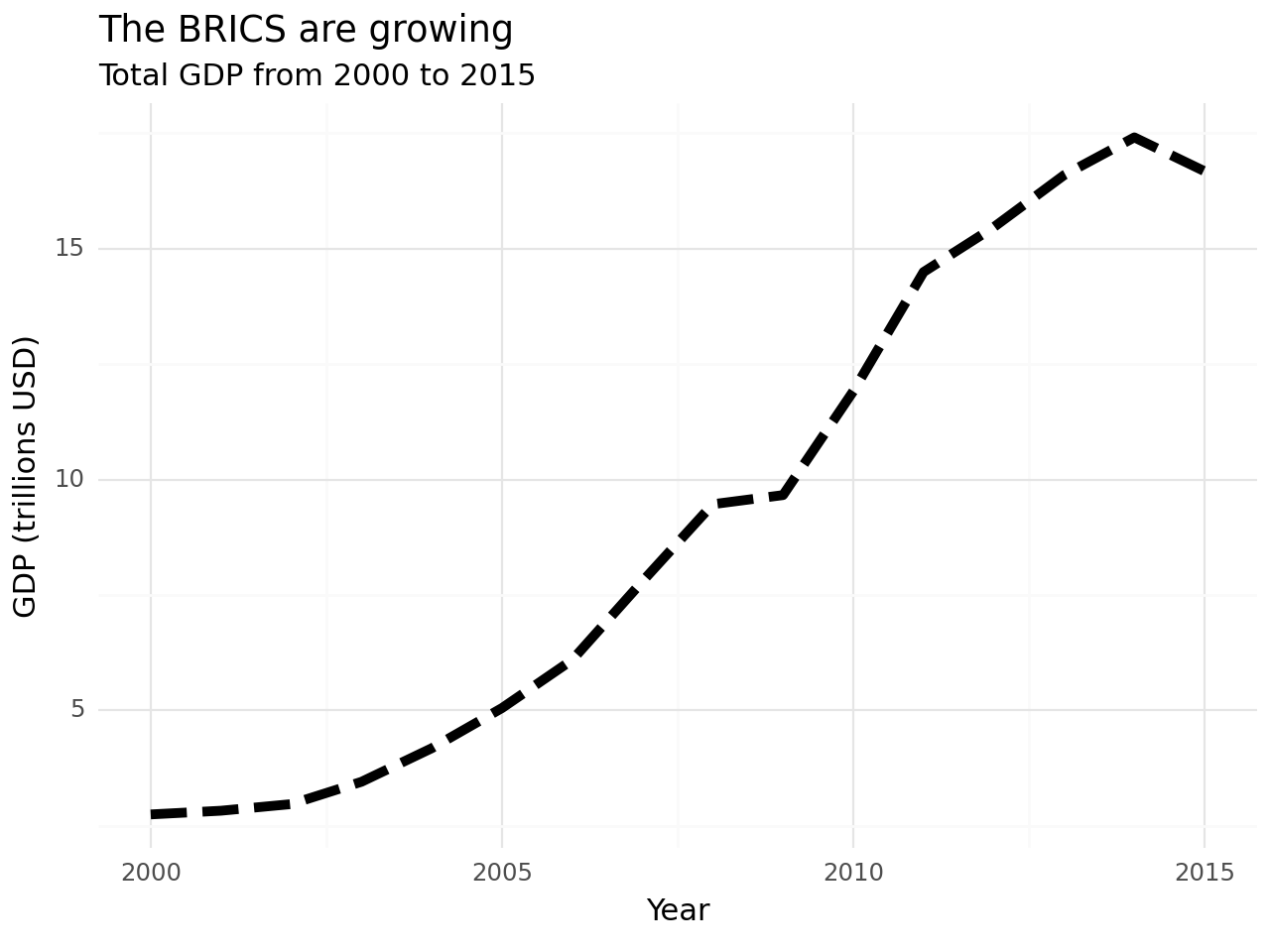
Visualise to observe any patterns – ‘seeing’ as a form of understanding
- What happens between 2005 and 2010?
(
 ggplot()
 + geom_line(total_gdp_brics, aes("year", "gdp"), size = 2, linetype = "dashed")
 + theme_minimal()
 + labs(x = "Year", y = "GDP (trillions USD)",
        title = "The BRICS are growing",
        subtitle = "Total GDP from 2000 to 2015")
 )
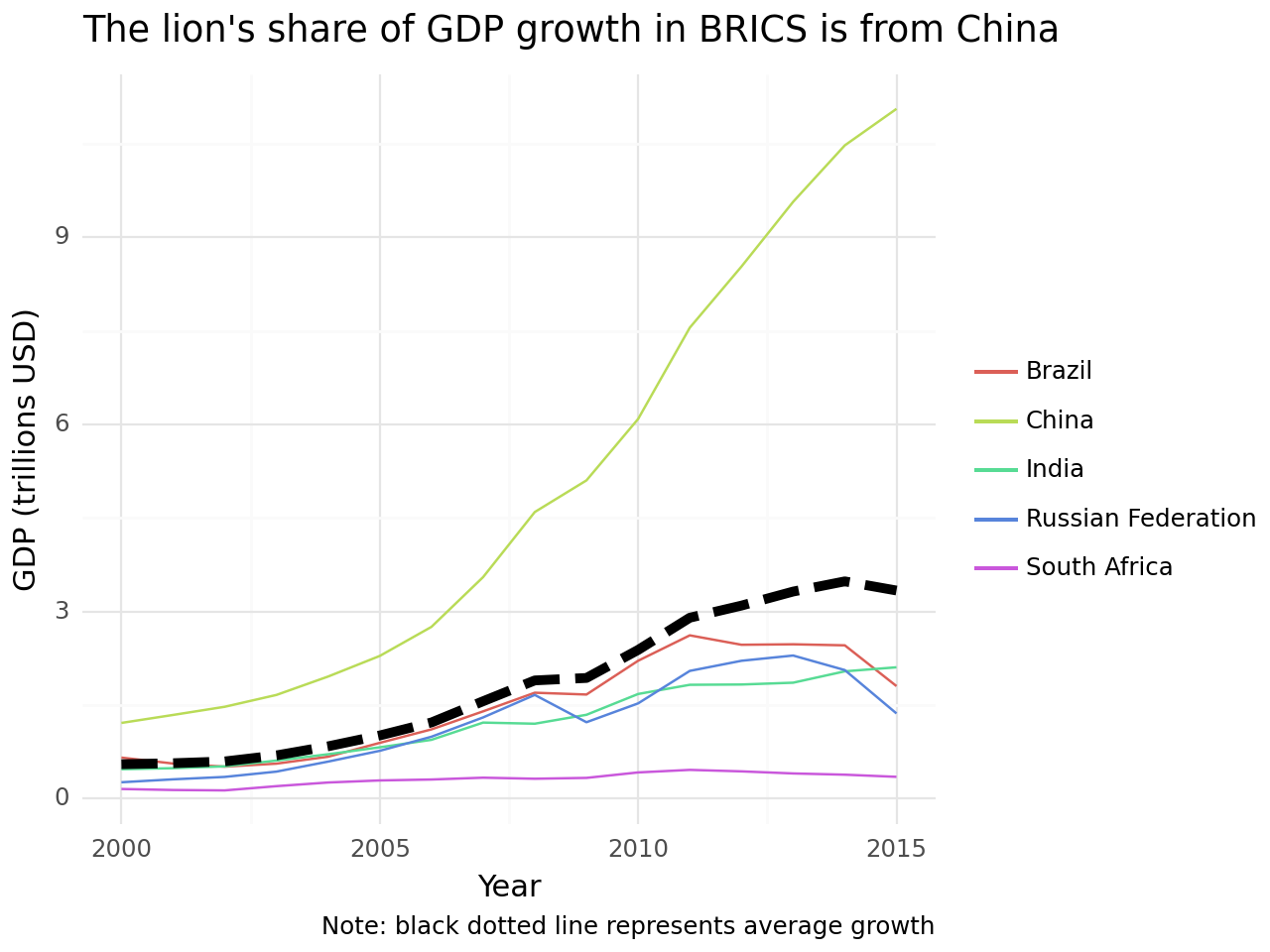
(
 ggplot()
 + geom_line(gdp_brics, aes("year", "gdp", colour = "country_name"))
 + geom_line(mean_gdp_brics, aes("year", "gdp"), size = 2, linetype = "dashed")
 + theme_minimal()
 + labs(x = "Year", y = "GDP (trillions USD)", colour = "",
        title = "The lion's share of GDP growth in BRICS is from China",
        caption = "Note: black dotted line represents average growth")
 )
Converting BRICS 2015 data to JSON
A convenience function to produce JSON from tables
gdp_brics| country_name | year | gdp | |
|---|---|---|---|
| 26 | Brazil | 2000 | 0.655448 |
| 41 | China | 2000 | 1.211332 |
| 88 | India | 2000 | 0.468396 |
| 160 | Russian Federation | 2000 | 0.259710 |
| 176 | South Africa | 2000 | 0.151753 |
| ... | ... | ... | ... |
| 3281 | Brazil | 2015 | 1.802212 |
| 3296 | China | 2015 | 11.061573 |
| 3343 | India | 2015 | 2.103588 |
| 3415 | Russian Federation | 2015 | 1.363482 |
| 3431 | South Africa | 2015 | 0.346710 |
80 rows × 3 columns
gdp_brics_2015 = gdp_brics.query("year == 2015").reset_index(drop = True).drop(columns = 'year')
gdp_brics_2015[["country_name"]] = gdp_brics_2015[["country_name"]].astype("string")
gdp_brics_2015[["gdp"]] = gdp_brics_2015[["gdp"]].astype("float")
print(gdp_brics_2015.info())

import json
gdp_brics_2015_json = gdp_brics_2015.to_json()

from pprint import pprint as pp
pp(gdp_brics_2015_json, depth=2)
<class 'pandas.core.frame.DataFrame'>
RangeIndex: 5 entries, 0 to 4
Data columns (total 2 columns):
# Column Non-Null Count Dtype
--- ------ -------------- -----
0 country_name 5 non-null string
1 gdp 5 non-null float64
dtypes: float64(1), string(1)
memory usage: 212.0 bytes
None
('{"country_name":{"0":"Brazil","1":"China","2":"India","3":"Russian '
'Federation","4":"South '
'Africa"},"gdp":{"0":1.8022122069,"1":11.0615726186,"2":2.10358836,"3":1.3634821822,"4":0.3467097905}}')JSON output
JSON notation has the same formatting structure as a Python ‘dictionary’
{
  "country_name": {
    "0": "Brazil",
    "1": "China",
    "2": "India",
    "3":"Russian Federation",
    "4":"South Africa"},
  "gdp":{"0":1.8022122069,
        "1":11.0615726186,
        "2":2.10358836,
        "3":1.3634821822,
        "4":0.3467097905}
}
Re-formatted
gdp_brics_2015_json = gdp_brics_2015.to_json(orient = "index")


from pprint import pprint as pp
pp(gdp_brics_2015_json, depth=2)
('{"0":{"country_name":"Brazil","gdp":1.8022122069},"1":{"country_name":"China","gdp":11.0615726186},"2":{"country_name":"India","gdp":2.10358836},"3":{"country_name":"Russian '
'Federation","gdp":1.3634821822},"4":{"country_name":"South '
'Africa","gdp":0.3467097905}}'){
"0": {
"country_name": "Brazil",
"gdp": 1.8022122069
},
"1": {
"country_name": "China",
"gdp": 11.0615726186
},
"2": {
"country_name": "India",
"gdp": 2.10358836
},
"3": {
"country_name":"Russian Federation","gdp":1.3634821822},
"4":{"country_name":"South Africa","gdp":0.3467097905}
}# print(
# gdp_brics.query("year == 2015").reset_index(drop = True).drop(columns = "year").to_json()
# )Converting BRICS 2010 data to HTML
A convenience function to produce HTML tables (you can embed these into your own web reports)
html = gdp_brics.query("year == 2010").reset_index(drop = True).drop(columns = "year").to_html()
html_op = os.path.join('DS101A_data', 'gdp_brics_2010.html')

with open(html_op, 'w') as html_file:
    html_file.write(html)

print(html)
<table border="1" class="dataframe">
<thead>
<tr style="text-align: right;">
<th></th>
<th>country_name</th>
<th>gdp</th>
</tr>
</thead>
<tbody>
<tr>
<th>0</th>
<td>Brazil</td>
<td>2.208838</td>
</tr>
<tr>
<th>1</th>
<td>China</td>
<td>6.087192</td>
</tr>
<tr>
<th>2</th>
<td>India</td>
<td>1.675616</td>
</tr>
<tr>
<th>3</th>
<td>Russian Federation</td>
<td>1.524917</td>
</tr>
<tr>
<th>4</th>
<td>South Africa</td>
<td>0.417364</td>
</tr>
</tbody>
</table>g7 = ["Canada", "France", "Germany", "Italy", "Japan", "United Kingdom", "United States"]
gdp_g7 = gdp_long.query("country_name in @g7")
#gdp_g7["gdp"] = gdp_g7["gdp"].astype(float) / 1e12
gdp_g7.loc[:,"gdp"] = gdp_g7["gdp"].astype(float) / 1e12
print(gdp_g7) country_name year gdp
35 Canada 2000 0.744773
67 France 2000 1.365640
72 Germany 2000 1.947982
95 Italy 2000 1.146677
97 Japan 2000 4.968359
... ... ... ...
3327 Germany 2015 3.357586
3350 Italy 2015 1.836638
3352 Japan 2015 4.444931
3460 United Kingdom 2015 2.927911
3461 United States 2015 18.295019
[112 rows x 3 columns]total_gdp_g7 = gdp_g7.groupby("year", as_index = False)["gdp"].sum()
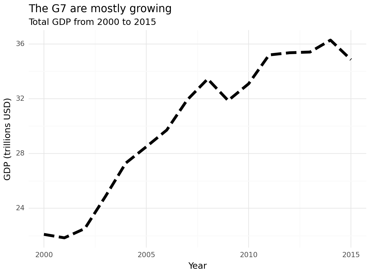
mean_gdp_g7 = gdp_g7.groupby("year", as_index = False)["gdp"].mean()(
ggplot()
+ geom_line(total_gdp_g7, aes("year", "gdp"), size = 2, linetype = "dashed")
+ theme_minimal()
+ labs(x = "Year", y = "GDP (trillions USD)",
title = "The G7 are mostly growing",
subtitle = "Total GDP from 2000 to 2015")
)
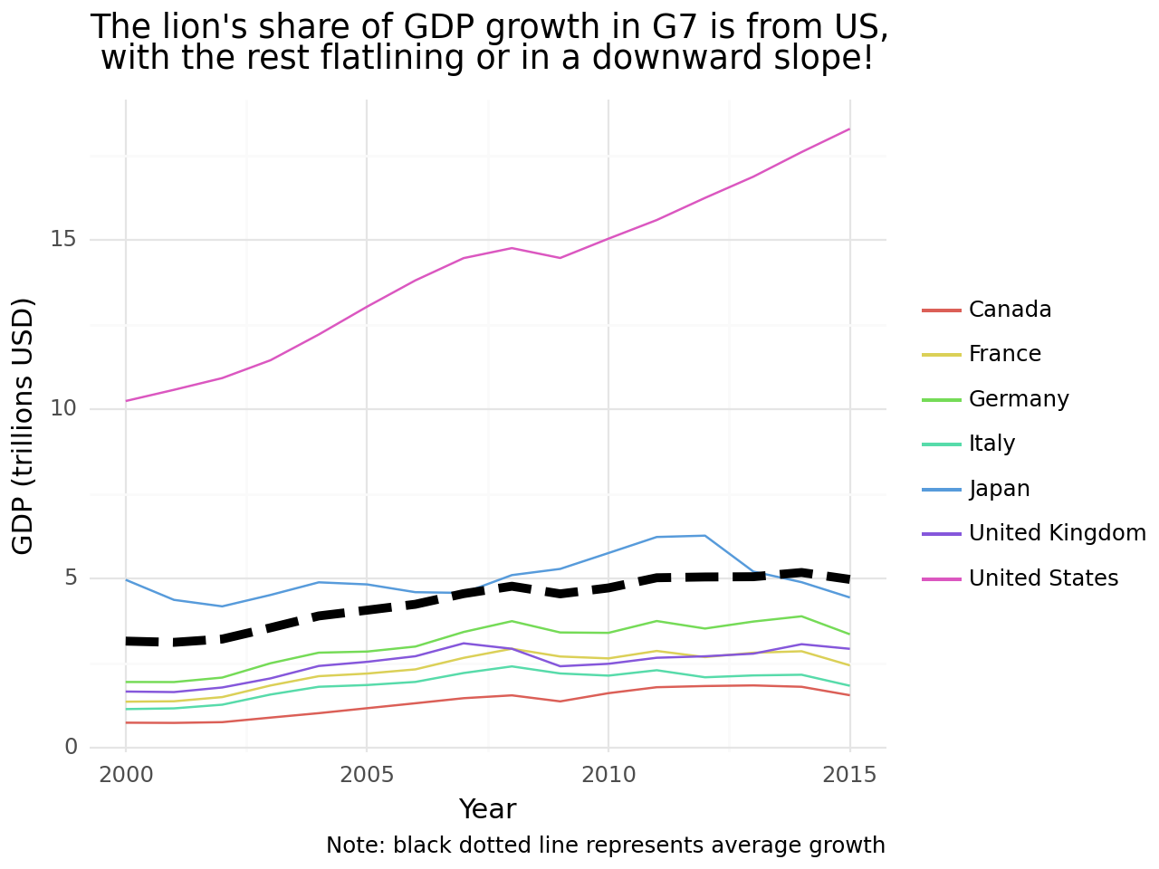
(
 ggplot()
 + geom_line(gdp_g7, aes("year", "gdp", colour = "country_name"))
 + geom_line(mean_gdp_g7, aes("year", "gdp"), size = 2, linetype = "dashed")
 + theme_minimal()
 + labs(x = "Year", y = "GDP (trillions USD)", colour = "",
        title = "The lion's share of GDP growth in G7 is from US,\n with the rest flatlining or in a downward slope!",
        caption = "Note: black dotted line represents average growth")
 )
