💻 Week 07 - Class Roadmap (90 min)

2023/24 Autumn Term

Welcome to the sixth class of the course!

As mentioned during the lecture on Monday, today, we will be exploring the UCI Diagnostic Wisconsin Breast Cancer Database (Wolberg and Street 1995) and testing a few classification algorithms on it.

In this class, you’ll need to run code a Jupyter Notebook: it’s up to you to decide whether you want to open a new Jupyter Notebook in Nuvolos, Google Colab or simply in VSCode.

Step 1 - Download the dataset (~5min)

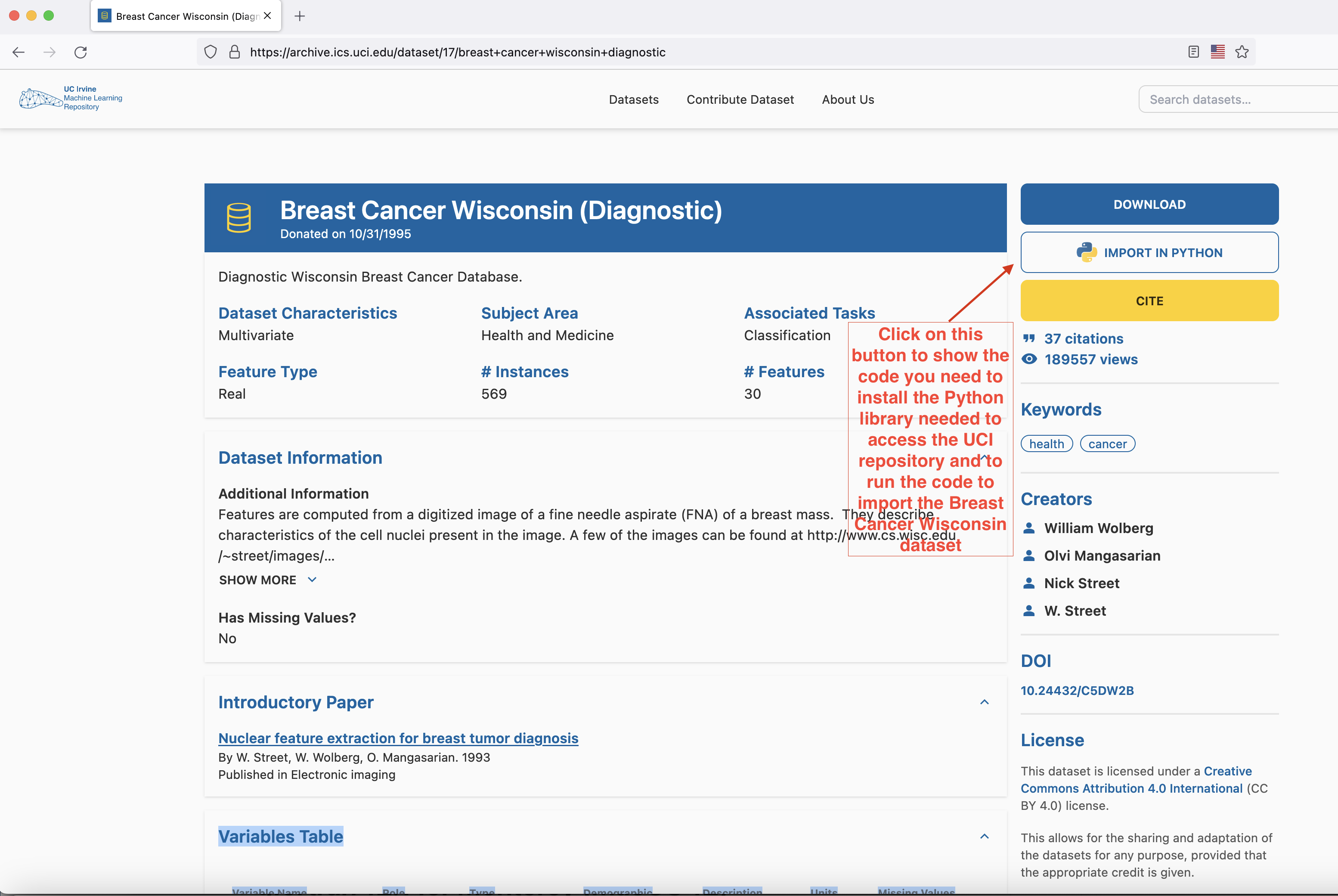
Head to here to download the dataset. The easiest way to proceed is to open a Jupyter Notebook file (either through Google Colab or through VSCode) and follow the instructions of the popup that shows up when you press the IMPORT IN PYTHON button on the page.

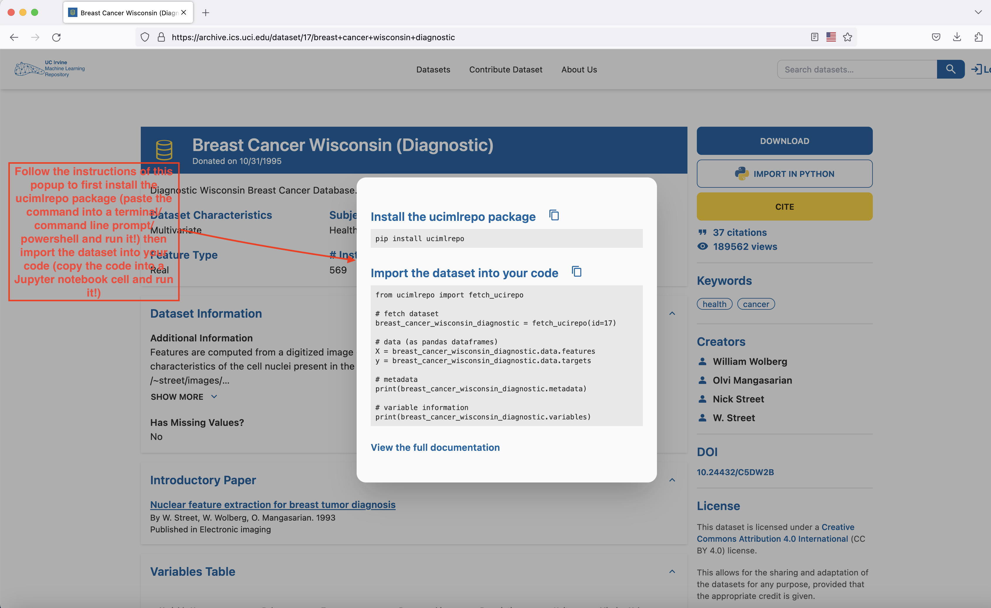
1. Install the ucimlrepo package with the pip install ucimlrepo command (run this command either on a cell in your Google Colab notebook or open Terminal/Command line prompt/Power Shell in your laptop, paste this command into it and run it)
2. Copy the block of code that appears in the Import the dataset into your code section of the popup into a cell of your Google Colab or VSCode notebook and run it. The dataset has now been loaded and you’re ready to proceed to the next part of the lab

Step 2 - Basic data exploration and processing (~40min)

Before you’re ready to do anything with the data, you need to explore it a bit to understand its main features. that’s the objective of this part of the class. The full information about the dataset can be found here.

Tip

In this dataset, the independent variables and the dependent variable are not part of a single dataframe but are two distinct dataframes contained in distinct data structures.

If you need to access the dataframe corresponding to the independent variables in the dataset, you need to get the breast_cancer_wisconsin_diagnostic.data.features variable and if you need to access the dependent variable, then the variable you need to access is breast_cancer_wisconsin_diagnostic.data.targets.

1. With the help of the code from Week 3 and Week 5, can you:
   • get basic information about your dataset (e.g column names, data types of each column, the number of non-null entries per column)
   • visualise the missing values per column?

💭 Do we need to do any missing value imputation for this dataset? Do we need to clean up column names?

2. Now we need to check how many elements of each class we have our data:

• First, you need to retrieve the target variable and convert it into a list type. Use this code to do so:

     target_values=breast_cancer_wisconsin_diagnostic.data.targets.values.tolist()

  (if you want to visualise the result of the command you’ve just typed and run, you can run either this command:

    target_values

  or this one

    print(target_values)

  in a separate code block from the previous one )

• then, you need to flatten target_values (this is a list of lists and needs to become a list so we can count its elements; we’ll use a predefined function from the standard itertools library to do that) and then count its elements again using a predefined function this time from the standard collections library.
  In summary, simply use this code to count the elements in target_values:

    from itertools import chain
    from collections import Counter
    counts=Counter(chain(*target_values))
    for  k in counts.keys():
         print("---------------------------\ntarget value:", k, '\nnumber of elements for target value',k,":",counts[k],'\nproportion in data:',counts[k]/len(target_values))

🩻 What do you notice?

🧑‍🏫 TEACHING MOMENT: Your class teacher will explain:

• the notion of imbalanced data
• why this is a problem
• ways to overcome this

3. We will make the dataset balanced by using an oversampling technique called SMOTE (Synthetic Minority Over-sampling Technique)(Chawla et al. 2002):

   • To do this, you will need to have imbalanced-learn library installed so run the conda install imbalanced-learn if you are running your code in VSCode (if you are using Google Colab, the library is already pre-installed so you can skip this install command).

   • Then run this code in a new code block:

        from imblearn.over_sampling import SMOTE
        oversample=SMOTE()
        X,y=oversample.fit_resample(breast_cancer_wisconsin_diagnostic.data.features,breast_cancer_wisconsin_diagnostic.data.targets)

   • Now, check the number of elements for each class in your new (oversampled) dataset:

      target_values=y.values.tolist()
      l=list(chain.from_iterable(target_values))
      counts=Counter(chain(*target_values))
      for k in counts.keys():
          print("---------------------------\ntarget value:", k, '\nnumber of elements for target value',k,":",counts[k],'\nproportion in data:',counts[k]/len(target_values))

🩻 What do you notice?

4. Before we proceed, let’s check the correlations between our dataset variables

   import pandas as pd
   import numpy as np
   import math

   #Data visualization
   import matplotlib.pyplot as plt
   import seaborn as sns
   %matplotlib inline
   colors = ['#c1121f','#669bbc', '#f4d35e', '#e9724c', '#ffc857']
   plt.style.use('seaborn-v0_8-white')
   plt.rc('figure', figsize=(12,8))
   plt.rc('font', size=18)
   plt.rc('axes', labelsize=14, titlesize=14)
   plt.rc('legend', fontsize=14)
   plt.rc('xtick', labelsize=10)
   plt.rc('ytick', labelsize=10)
 
   data=pd.concat([X,y],axis=1)
   plt.figure(figsize=(25,25))

   heatmap_colors = [colors[1], '#d6d5c9', colors[0]]

   corr = data.corr()
   mask = np.triu(np.ones_like(corr, dtype=bool))

   sns.heatmap(data.corr(),
            mask=mask,
            center=0,
            annot=True,
            fmt='.2f',
            cmap=heatmap_colors,
            square=True,
            linewidths=.2,
            cbar_kws={"shrink": .6})

    plt.title('Features Correlation Matrix Heatmap', fontsize=18);

🩻 What do you notice?

We drop all unnecessary columns (i.e columns exhibiting strong correlations with other in the dataset) and plot the correlation heatmap for this new, reduced dataset:

   cleaned_data=data[['Diagnosis', 'radius1', 'texture1', 'smoothness1',
       'compactness1', 'symmetry1', 'fractal_dimension1',
       'radius2', 'texture2', 'smoothness2', 'compactness2',
       'symmetry2', 'fractal_dimension2']]
   plt.figure(figsize=(25,25))

   heatmap_colors = [colors[1], '#d6d5c9', colors[0]]

   corr = cleaned_data.corr()
   mask = np.triu(np.ones_like(corr, dtype=bool))

   sns.heatmap(cleaned_data.corr(),
            mask=mask,
            center=0,
            annot=True,
            fmt='.2f',
            cmap=heatmap_colors,
            square=True,
            linewidths=.2,
            cbar_kws={"shrink": .6})

   plt.title('Features Correlation Matrix Heatmap', fontsize=18);

5. Let’s now split our dataset in two: a training set (on which we’ll train our models) and a test set (on which we’ll test their performance). To do that use the code below:

# Split the data into training and testing sets
from sklearn.model_selection import train_test_split
X = cleaned_data.drop(columns=['Diagnosis'])
y = cleaned_data['Diagnosis']

X_train, X_test, y_train, y_test = train_test_split(X, y, test_size=0.3, random_state=42)

This code is splitting the data into training and testing sets using the train_test_split function from the sklearn.model_selection module:

• The X and y variables are the input features and target variable (obtained by oversampling earlier), respectively.

• The test_size parameter specifies the proportion of the data that should be used for testing, in this case 30% (and 70% for the training set).

• The random_state parameter sets the seed for the random number generator, ensuring that the same split is obtained each time the code is run.

• The function returns four arrays: X_train and y_train are the training set, while X_test and y_test are the test set.

Part 3 - Exploring classification algorithms (~40min)

In this part, we’ll explore some of the classication algorithms we mentioned during the lecture on Monday.

1. We’ll first start with logistic regression:

   • we first need to import some important libraries:

      import statsmodels.api as sm
      import statsmodels.formula.api as smf

   • We need to prepare a parameter that is going to be used in the logistic regression function from the statsmodels library:

   
      # Logistic Regression Model
   
      # Create a string for the formula
      cols = cleaned_data.columns.drop('Diagnosis')
      formula = 'Diagnosis ~ ' + ' + '.join(cols)
      print(formula, '\n')

   • We run the model and report the results:

        # Run the model and report the results
        model = smf.glm(formula=formula, data=X_train, family=sm.families.Binomial())
        logistic_fit = model.fit()
     
        print(logistic_fit.summary())

   • We make predictions on unseen data using the model we’ve just trained:

      # predict the test data and show the first 10 predictions
      predictions = logistic_fit.predict(X_test)
      predictions[0:10]

   🐍 Can you show the 40th to the 100th prediction? (Hint: Python indices start at zero, so prediction number 1 is predictions[0] instead of predictions[1])

   We have now shown the probability of each element of the test of belonging to one class or another. To assign each element to a class, we need a probability cut-off point or threshold. Here, we set the threshold to 0.5 and assign to class “M” all elements whose probability is lower than 0.5 and to class “B” all elements with probability higher than 0.5.

   This is what this looks like translated in code:

      # Note how the values are numerical.
      # Convert these probabilities into nominal values and check the first 10 predictions again.
      predictions_nominal = [ "M" if x < 0.5 else "B" for x in predictions]
      predictions_nominal[0:10]

   Finally, we assess the performance of our model using the accuracy metric:

      from sklearn.metrics import accuracy_score
      # Calculate accuracy
      logistic_accuracy = accuracy_score(y_test, predictions_nominal)
      logistic_accuracy

   • Before we continue, we create a numerical encoding for our target variable (translating “M” to 0 and “B” to 1) and encode our target variables (in the training/test sets) as well as the predictions we produced with logistic regression with it (to ensure we can make comparisons with other models).

   
    # To avoid confusion, define your custom encoding mapping
    custom_encoding = {
         'M': 0,
         'B': 1
    }
   
    # Use a list comprehension to apply the custom encoding
    y_train_encoded = [custom_encoding[label] for label in y_train]
    y_test_encoded = [custom_encoding[label] for label in y_test]
   
    #Let's get the predictions from our logistic regression model encoded (we'll need that for comparisons with other models later)
   
    encoded_logistic_predictions=[custom_encoding[e] for e in predictions_nominal]
    encoded_logistic_predictions[0:10] #showing the first 10 predictions (encoded)

   🐍 Use this code to check your encoding:

   
      # To check you encoding
      # Create a dictionary to store the mapping
      encoding_mapping = {label: var for label, var in zip(y_train, y_train_encoded)}
   
      # Print the mapping
      for label, var in encoding_mapping.items():
          print(f"{label} corresponds to {var}")

2. Next, we move to decision trees and we follow a similar process to earlier in this code block (this time, the model fitting and training uses the sklearn library instead of the statsmodels library).

# Decision Tree classification
from sklearn.tree import DecisionTreeClassifier

# We define the model
dtcla = DecisionTreeClassifier(random_state=9)

# We train model
dtcla.fit(X_train, y_train_encoded)

# We predict target values
y_dt_predict = dtcla.predict(X_test)

print("first 10 predictions for decision tree model", y_dt_predict[0:10].tolist() ) #showing the first ten predictions

#how does that compare to logistic regression

print("first 10 predictions for logistic model",encoded_logistic_predictions[0:10])

Note that we also compare the first ten predictions of the decision tree model with those of the logistic regression model. How do they compare?

🐍 Can you show the 40th to the 100th prediction of both models? (Hint: Python indices start at zero, so prediction number 1 is predictions[0] instead of predictions[1]) How do they compare?

Finally, we assess the performance of our decision tree model using the accuracy metric:

```python
   accuracy = accuracy_score(y_test_encoded, y_dt_predict)
   accuracy
```

🩻 How does this accuracy score compare to that of the logistic regression?

3. Finally, we move to the SVM model and the principle is the same as before: we train the model on the training set using the appropriate sklearn function, summarise the results, show the first ten predictions and compare them to those of the two previous models.

     # SVM (Support Vector Machine) classification
     from sklearn.ensemble import BaggingClassifier
     from sklearn.multiclass import OneVsRestClassifier
     from sklearn.svm import SVC
   
     # We define the SVM model
     svmcla = OneVsRestClassifier(BaggingClassifier(SVC(C=10, kernel='rbf',random_state=9, probability=True), n_jobs=-1))
   
     # We train model
     svmcla.fit(X_train, y_train_encoded)
   
     # We predict target values
     y_svm_predict = svmcla.predict(X_test)
   
   
     print("first 10 predictions for SVM model", y_svm_predict[0:10].tolist() ) #showing the first ten predictions
   
     # how does it compare to the other two models
   
     print("first 10 predictions for decision tree model", y_dt_predict[0:10].tolist() ) #showing the first ten predictions
   
     print("first 10 predictions for logistic model",encoded_logistic_predictions[0:10])

   🐍 How do the different models compare? What if you compare the 40th to 100th predictions instead?

   We also, as usual, compute the accuracy of the SVM model:

   
   svm_accuracy = accuracy_score(y_test_encoded, y_svm_predict)
   svm_accuracy

   🐍 What happens to the predictions and/or accuracy value if you change the parameters of the SVM model (e.g kernel) - see here how to do that? What about when you tweak the parameters of the decision tree model (e.g max tree depth or criterion) - see here how to do that?

References

Chawla, N. V., K. W. Bowyer, L. O. Hall, and W. P. Kegelmeyer. 2002. “SMOTE: Synthetic Minority over-Sampling Technique.” Journal of Artificial Intelligence Research 16 (June): 321–57. https://doi.org/10.1613/jair.953.

Wolberg, Mangasarian, William, and W. Street. 1995. “Breast Cancer Wisconsin (Diagnostic).” UCI Machine Learning Repository.