🗓️ Week 05:
Support Vector Machines (SVM)

Non-linear algorithms

Dr. Jon Cardoso-Silva and Dr. Stuart Bramwell

@LSEDataScience

10/28/22

What we will cover today

• Support Vector Machines
• Example: Iris data
• Overfitting
• Cross-validation* for the rescue!
• Tips for Summative Problem Set 01
• Thank you!

Support Vector Machines

Support Vector Machines for Classification

• Considered one of the best out-of-the-box classifiers (ISLR)
• Able to accommodate non-linear decision boundaries

Building Intuition: the Hyperplane

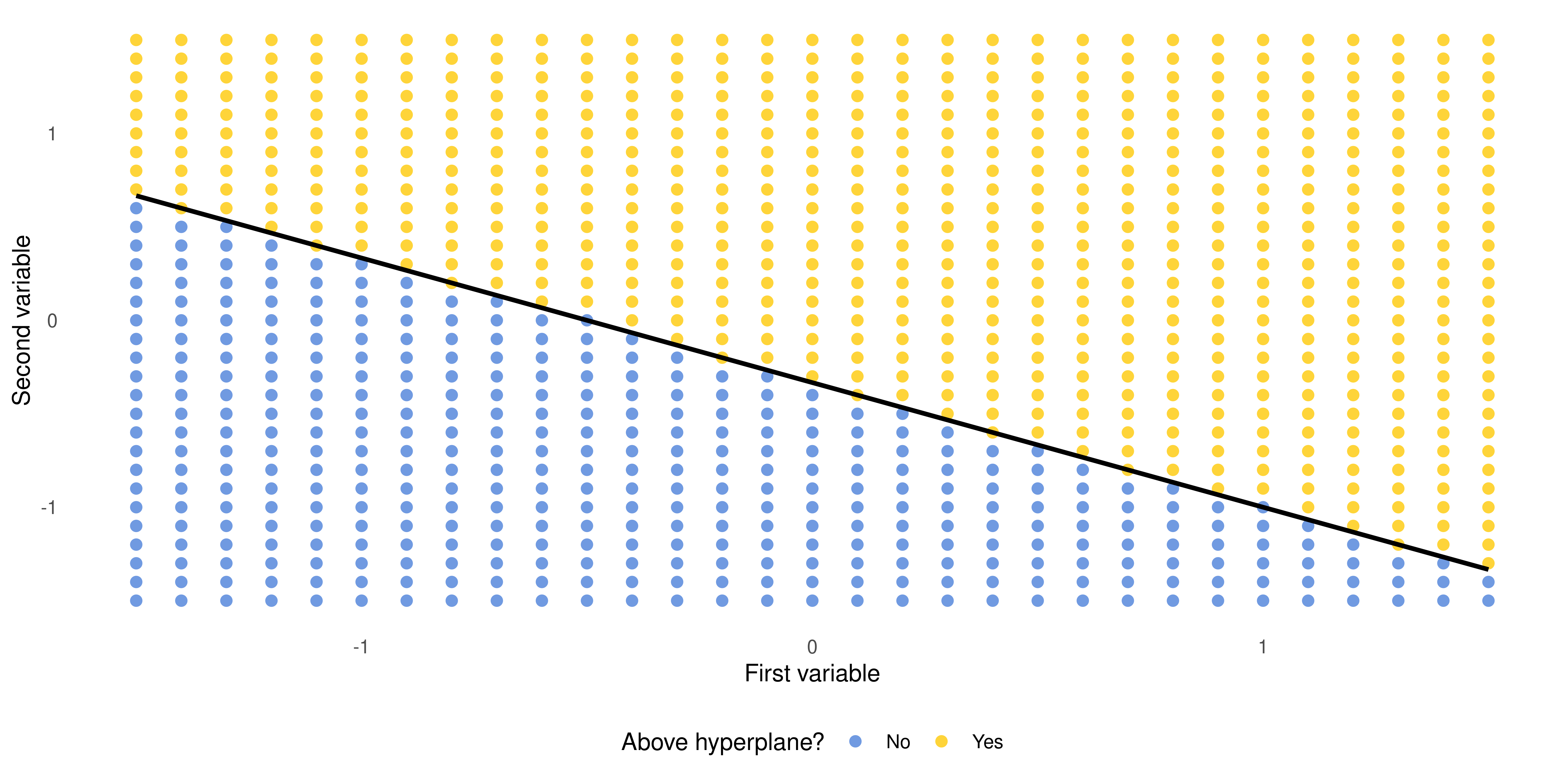
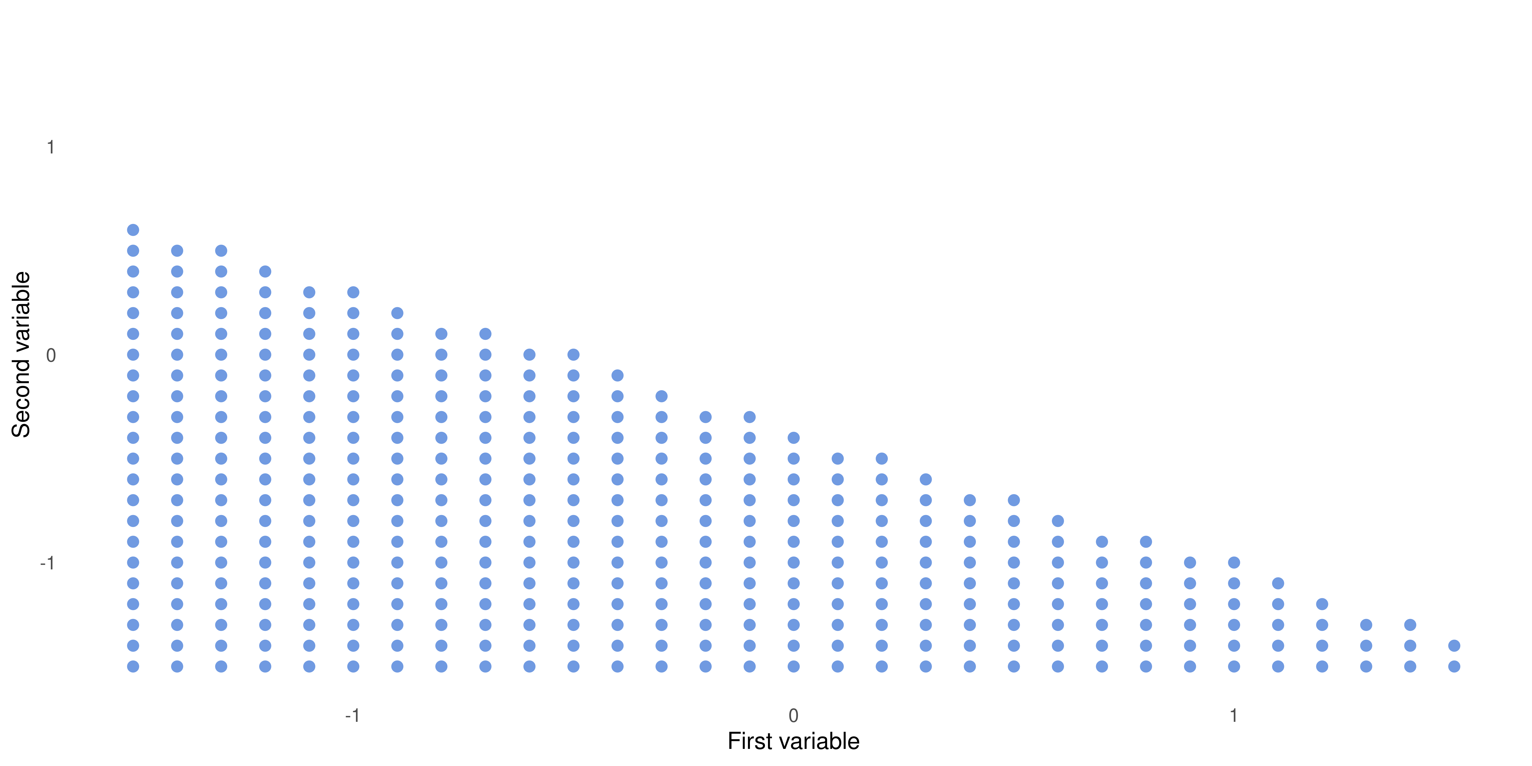
Building Intuition: the Hyperplane (cont.)

When \(1 + 2x_1 + 3x_2 < 0\)

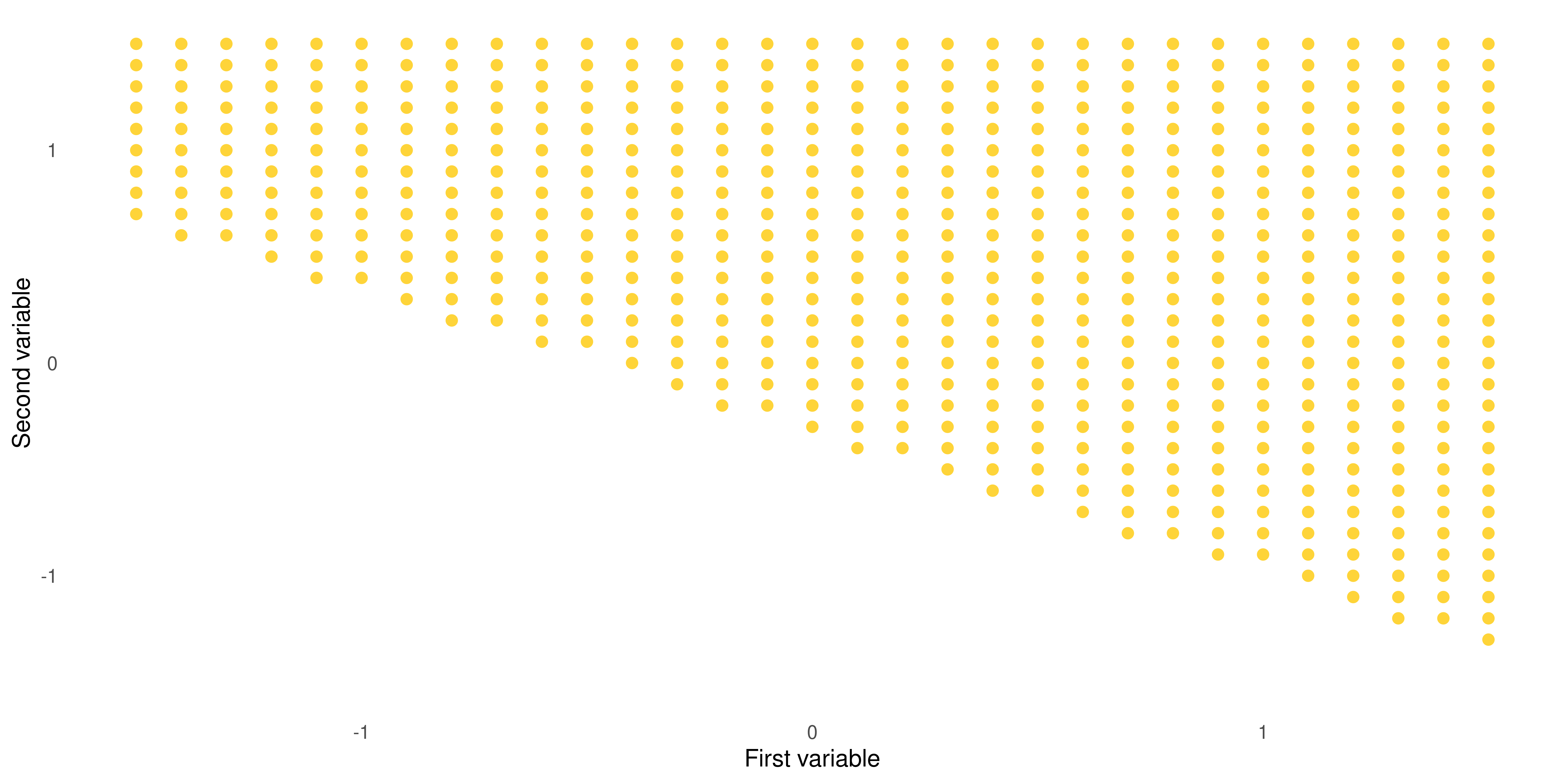
Building Intuition: the Hyperplane (cont.)

When \(1 + 2x_1 + 3x_2 > 0\)

Building Intuition: the Hyperplane (cont.)

When \(1 + 2x_1 + 3x_2 = 0\)

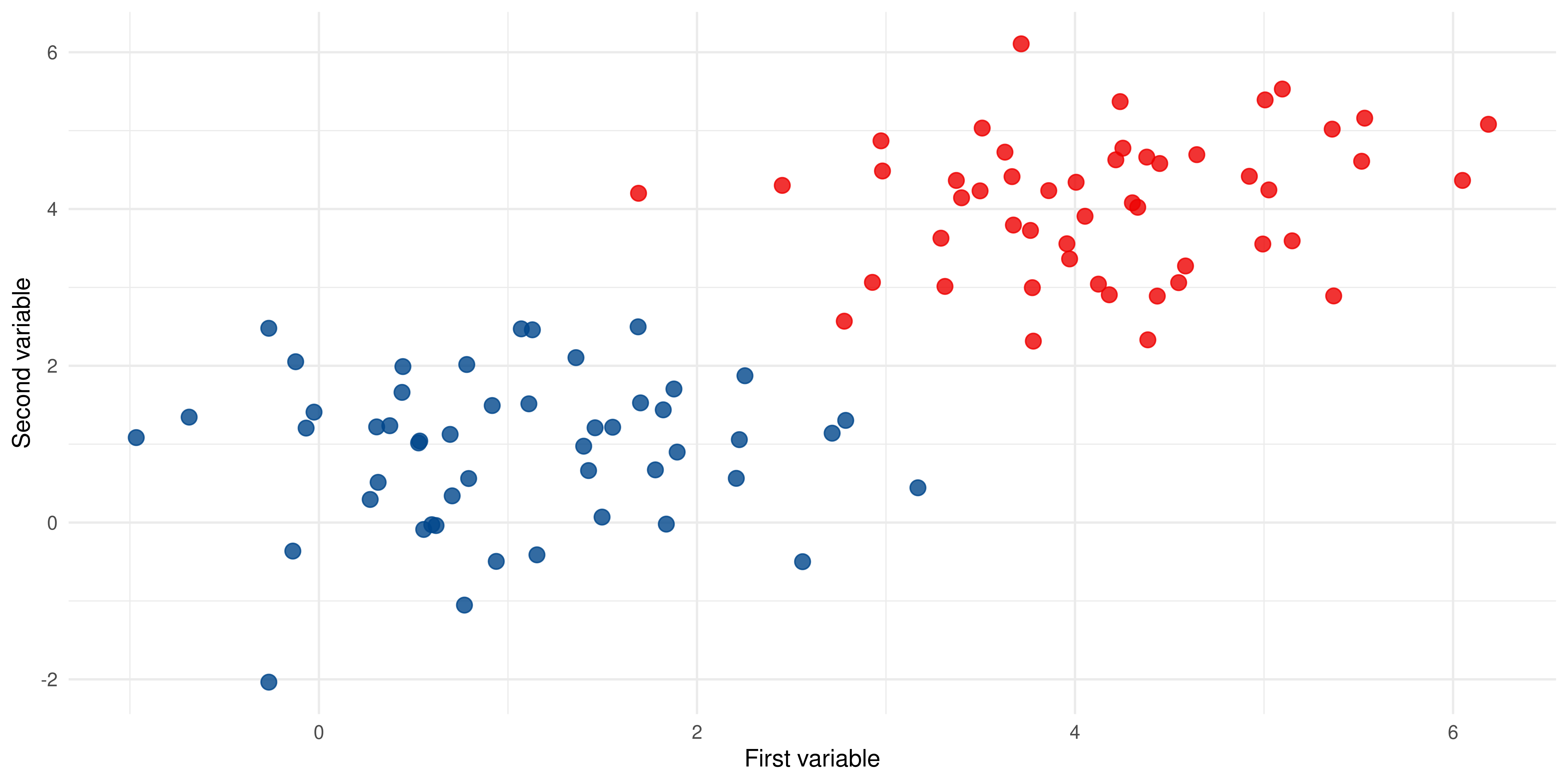
The Maximal Marginal Classifier

The linearly separable case:

Identifying support vectors

The SV’s represent the so-called support vectors:

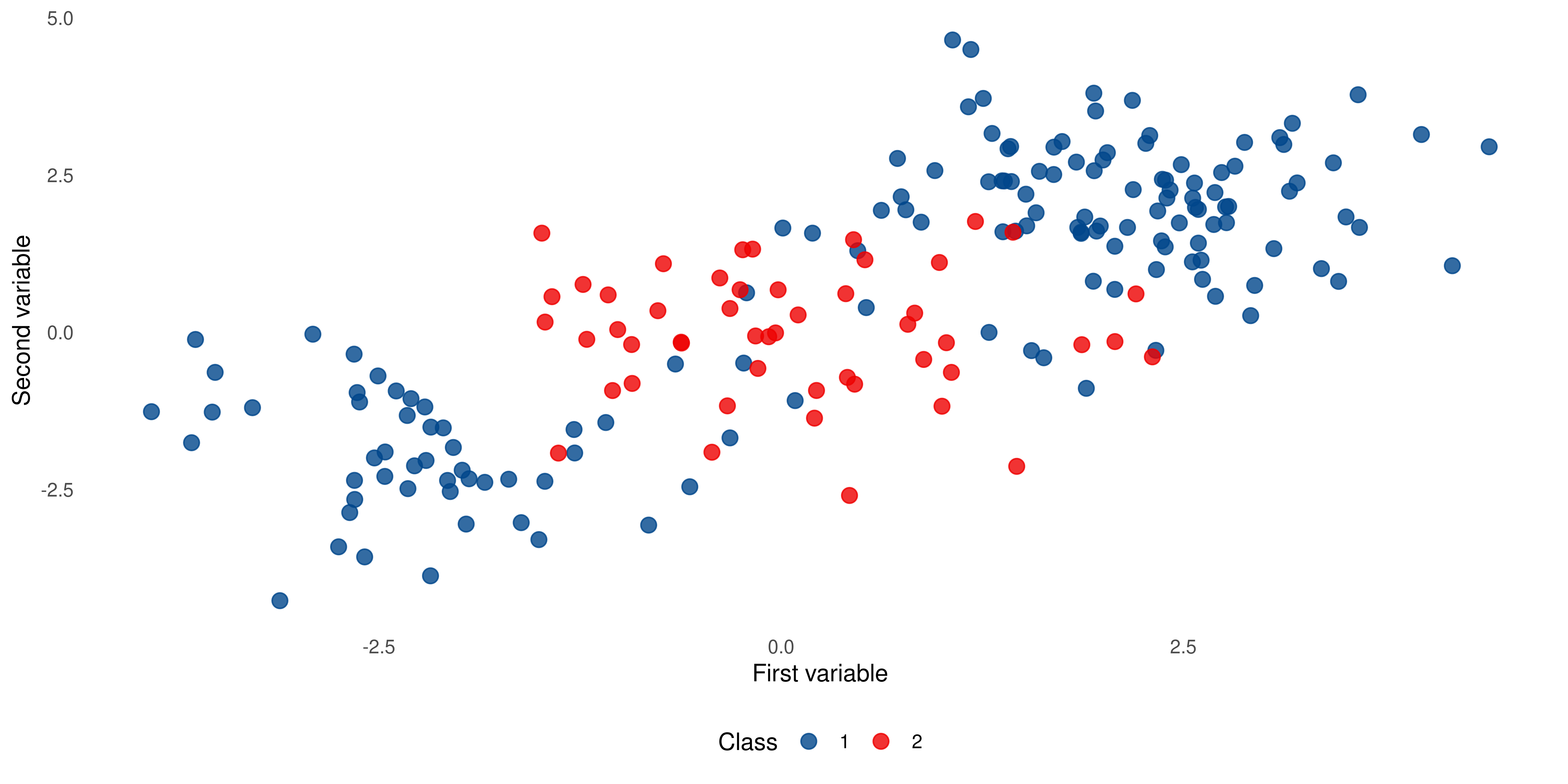
When data is not linearly separable

Suppose we have a case that is not linearly separable like this. We have two classes but class 1 is “sandwiched” in between class 2.

Enter support vector machines

Let’s start with a (linear) support vector classifier function

\[ f(x) = \beta_0 + \sum_{i\in\mathcal{S}}^{} \alpha_i\left\langle x_i, x_{i'} \right\rangle \]

A couple of points:

• \(\left\langle x_i, x_{i'} \right\rangle\) is the inner product ¹ of two observations
• \(\alpha_i\) is a parameter fitted for all pairs of training observations
• \(i\in\mathcal{S}\) indicates observations that are support vectors (all other observations are ignored by setting all \(\alpha_i \notin \mathcal{S}\) to zero.)

1. Read about inner products

Enter support vector machines (cont.)

• We can replace \(\left\langle x_i, x_{i'} \right\rangle\) with a of the form \(K(x_i, x_{i'})\) where \(K\) is a kernel.

Two well-known kernels:

• Polynomial \(K(x_i, x_{i'}) = (1 + \sum_{j = 1}^{p} x_{ij}x_{i'j})^d\) where \(d > 1\).
• Radial or “Gaussian” \(K(x_i, x_{i'}) = \text{exp}(-\gamma\sum_{j=1}^{p}(x_{ij}-x_{i'j})^2)\) where \(\gamma\) is a positive constant.

Example: Iris data

  Sepal.Length Sepal.Width Petal.Length Petal.Width Species
1          5.1         3.5          1.4         0.2  setosa
2          4.9         3.0          1.4         0.2  setosa
3          4.7         3.2          1.3         0.2  setosa
4          4.6         3.1          1.5         0.2  setosa
5          5.0         3.6          1.4         0.2  setosa
6          5.4         3.9          1.7         0.4  setosa

SVM with Linear Kernel

SVM with Polynomial Kernel

SVM with Sigmoid Kernel

SVM with Radial Kernel

Source Code

Tip

• Use the code below to replicate the plot from the previous slide.
• Found a bug? Report it on Slack.

library(datasets)   # to load the iris  data
library(tidyverse)  # to use things like the pipe (%>%), mutate and if_else
library(ggsci)      # just for pretty colours! It enables functions scale_fill_lancet() and scale_colour_lancet().
library(e1071)      # to load the SVM algorithm
data(iris)          # load the dataset `iris`

# Train the model! change the parameter `kernel`. It accepts 'linear', 'polynomial', 'radial' and 'sigmoid'
model <- svm(Species ~ Sepal.Length + Sepal.Width, data = iris, kernel = 'linear')

# Generate all possible combinations of Sepal.Length and Sepal.Width
kernel.points <- crossing(Sepal.Length = seq(4, 8, 0.1), Sepal.Width = seq(2, 5, 0.1)) %>%  mutate(pred = predict(model, .))

# Create a dataframe just for plotting (with predictions)
plot_df <- iris %>% mutate(pred=predict(model, iris), correct = if_else(pred == Species, TRUE, FALSE))

plot_df %>%   
  ggplot() +
  geom_tile(data = kernel.points, aes(x=Sepal.Length, y=Sepal.Width, fill = pred), alpha = 0.25) +
  geom_point(aes(x=Sepal.Length, y=Sepal.Width, colour = Species, shape = correct), size = 4) +
  scale_shape_manual(values = c(4, 1)) +
  scale_colour_lancet() +
  scale_fill_lancet() +
  theme_minimal() +
  theme(panel.grid = element_blank(), legend.position = 'bottom', plot.title = element_text(hjust = 0.5)) +
  labs(x = 'Sepal.Length', y = 'Sepal.Width', fill = 'Species', colour = 'Species', shape = 'Correct prediction?',
       title = sprintf('Overall Training Accuracy = %.2f %%', 100*(sum(plot_df$correct)/nrow(plot_df))))

Overfitting

Overfitting illustrated

Simple models can sometimes be better than complex models.

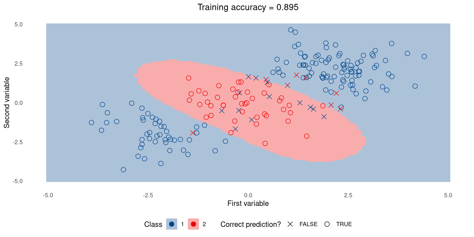
Simple model on training set

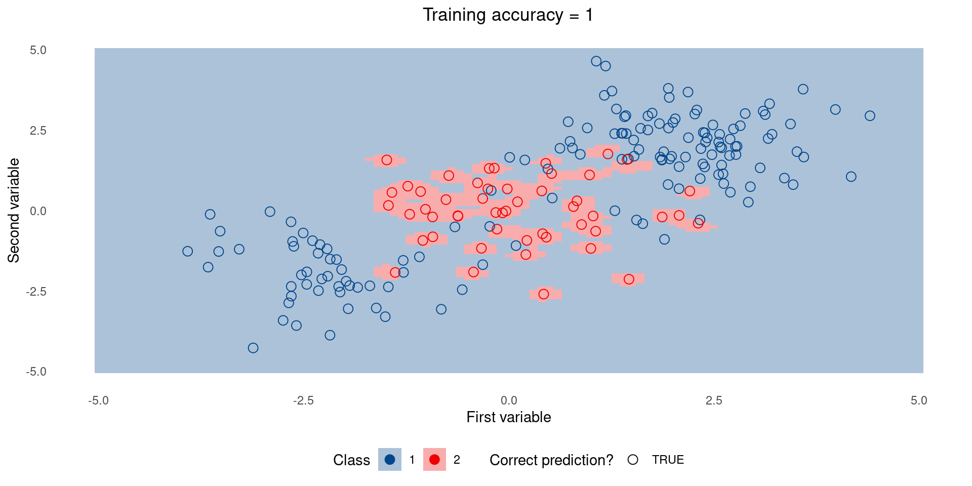
Complex model on training set

Now let’s create some testing data

Look what happens when I set a different seed (nothing else changes) to construct a test set.

Simple model on test set

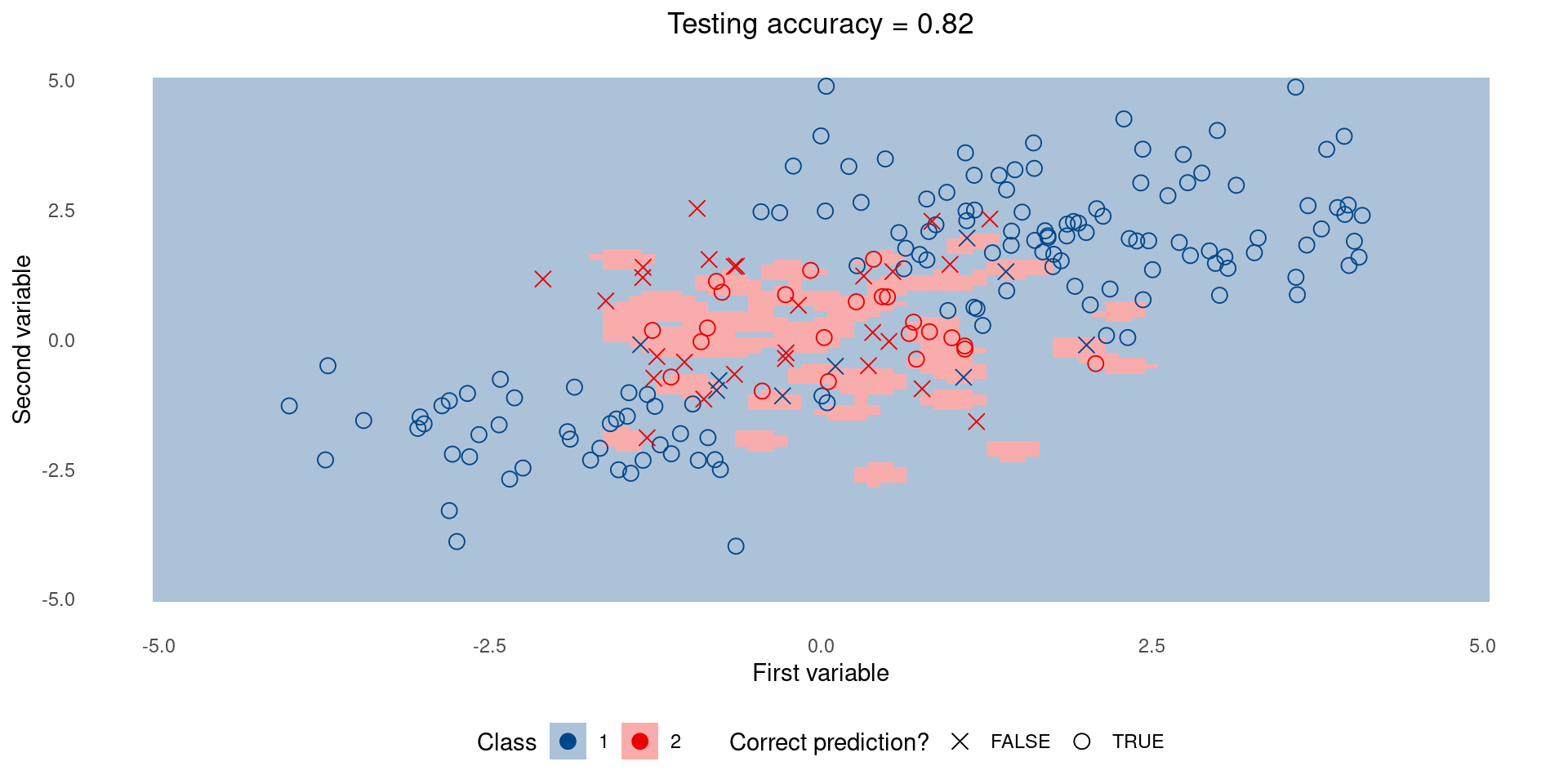
Complex model on test set

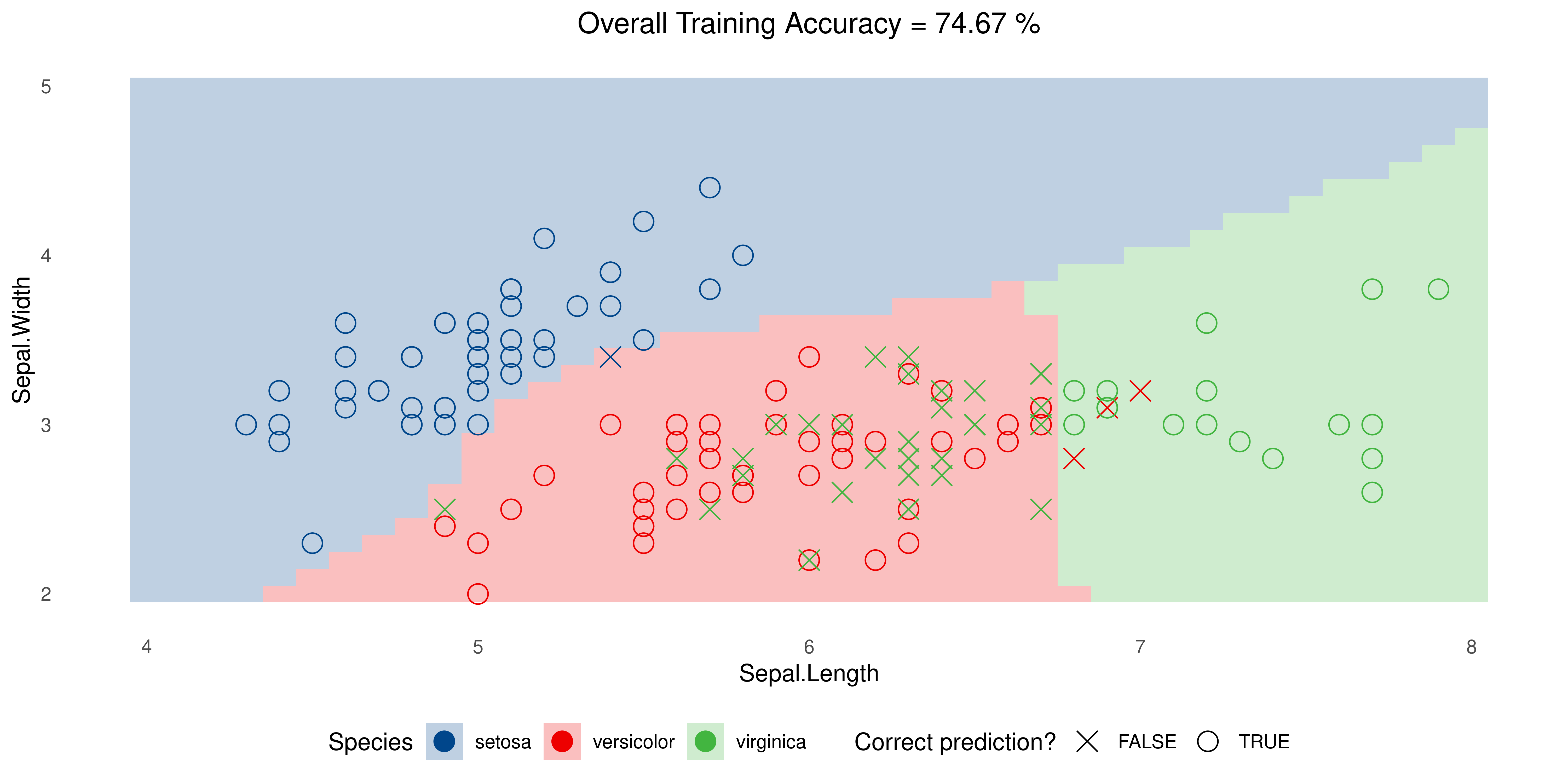
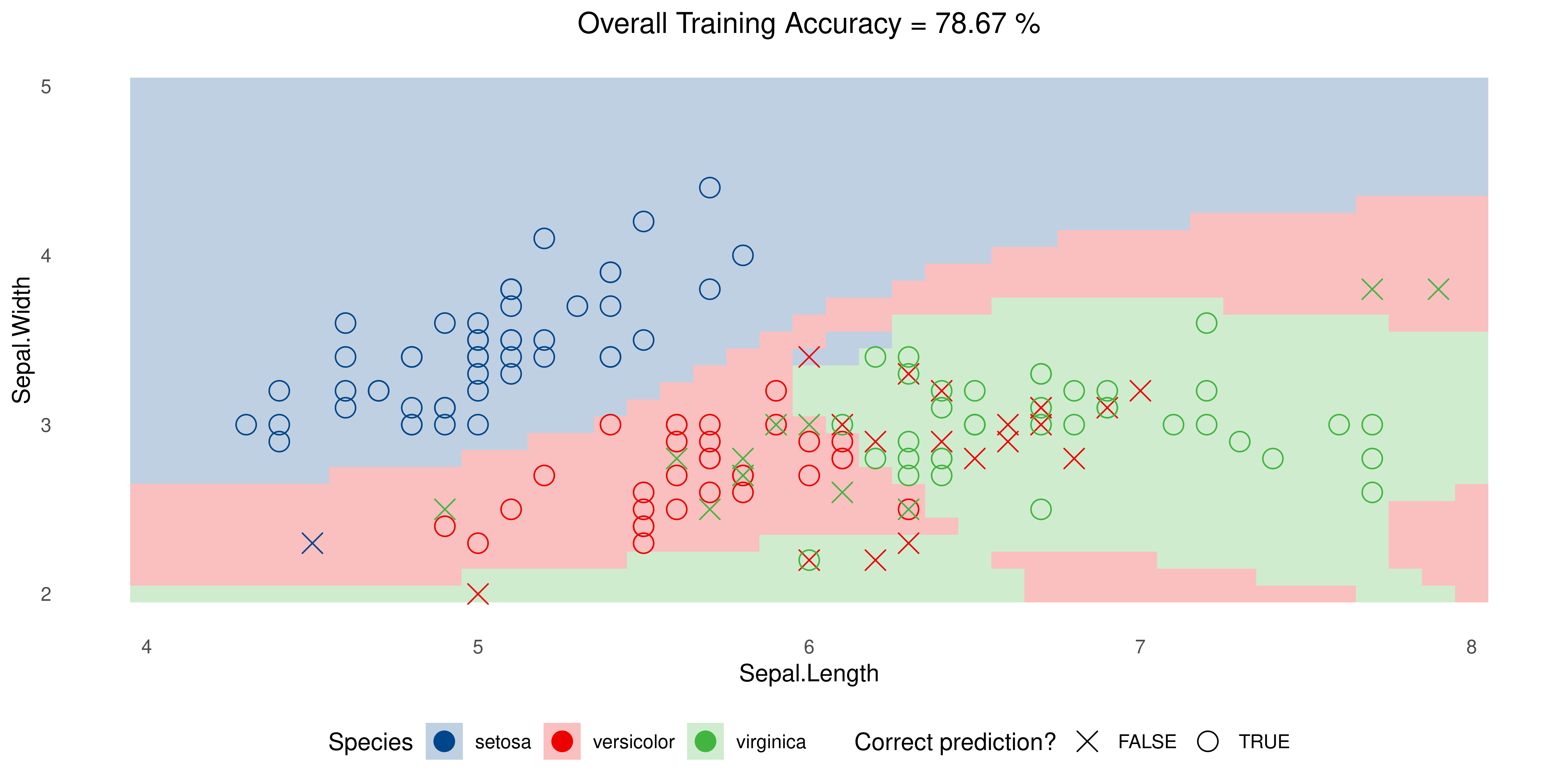
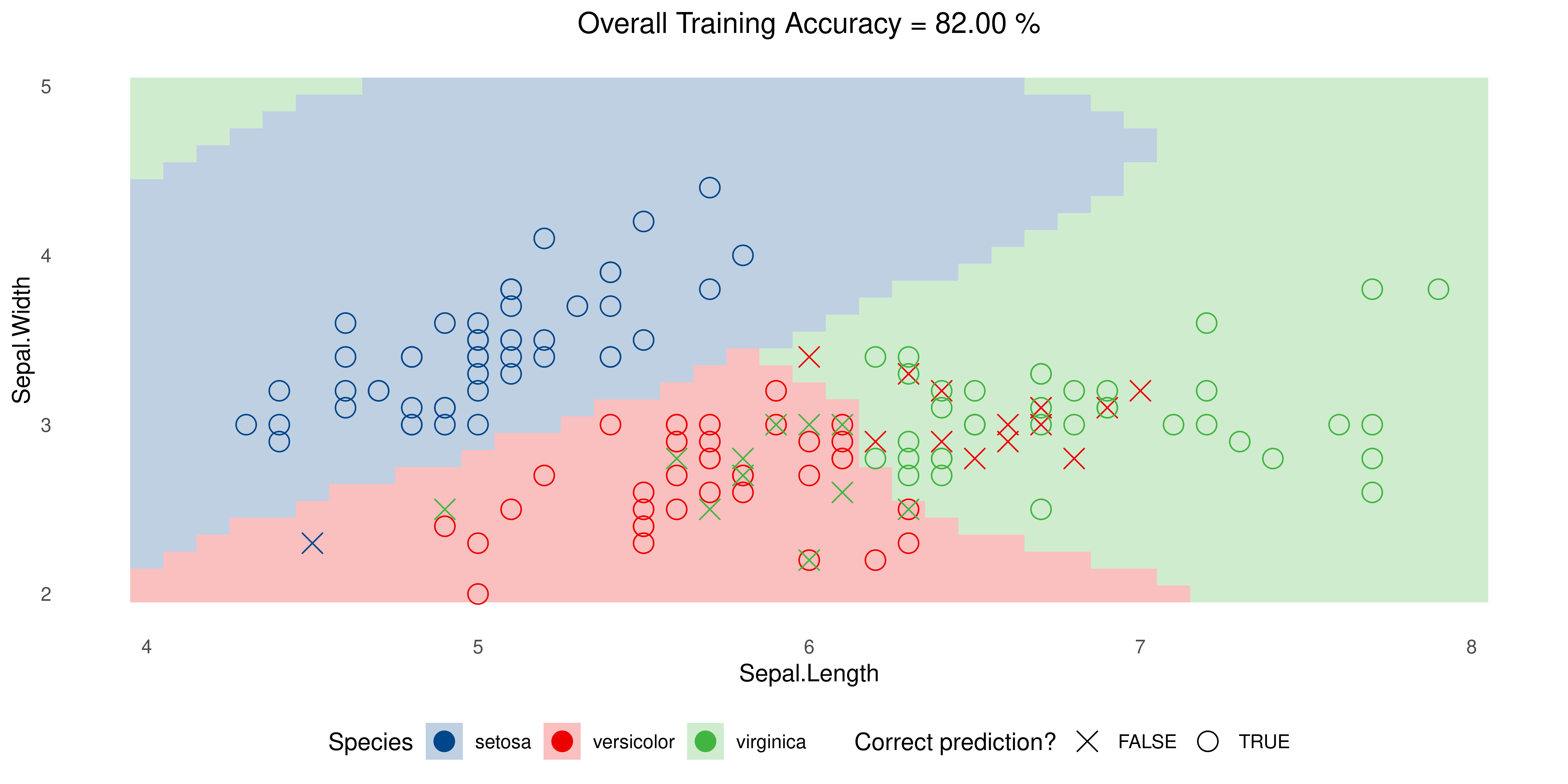
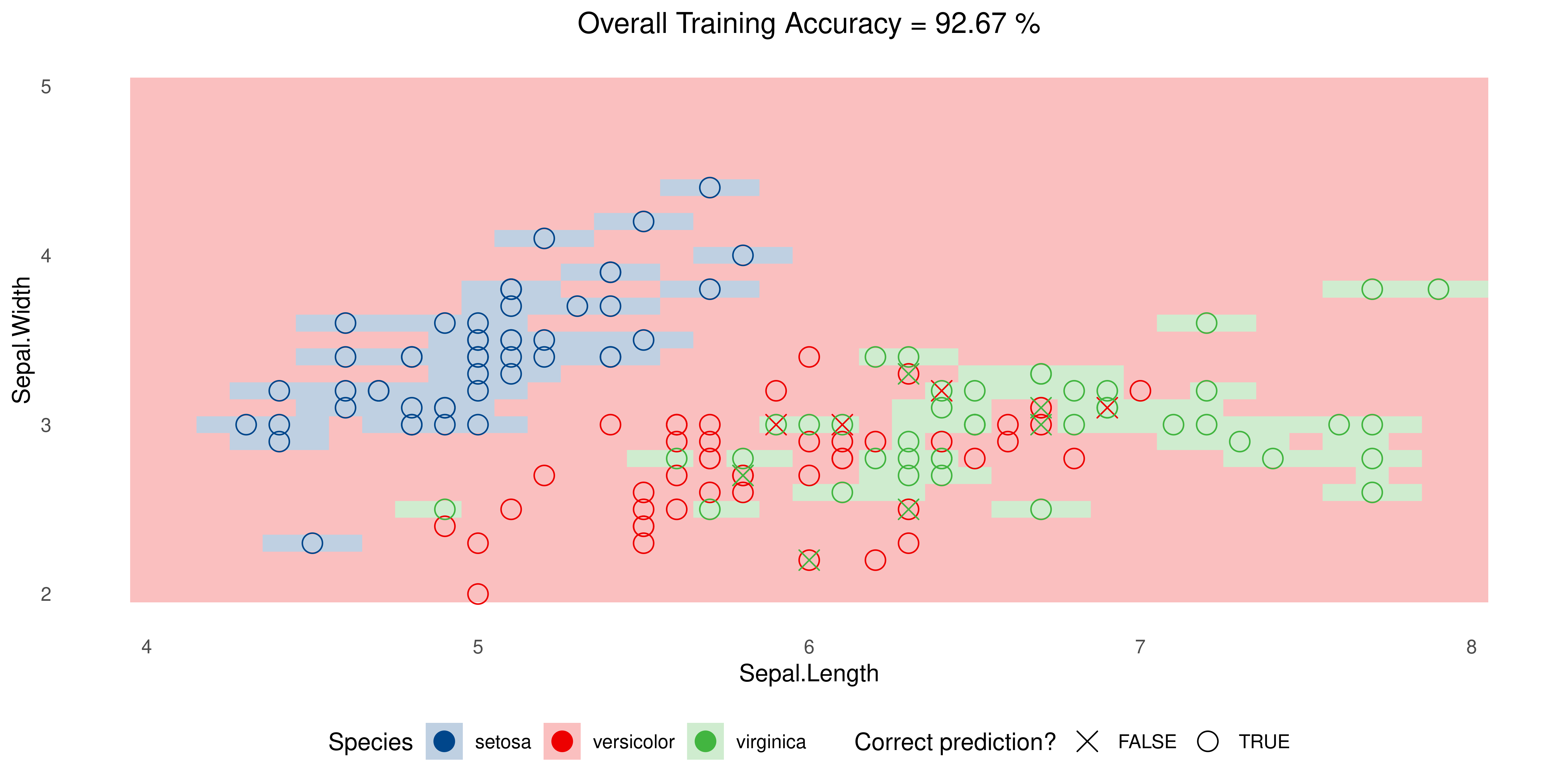
Back to iris

SVM with Radial Kernel but tweaking parameters, namely cost and gamma:

Source Code

Tip

• The only difference is that we added gamma and cost:

library(datasets)   # to load the iris  data
library(tidyverse)  # to use things like the pipe (%>%), mutate and if_else
library(ggsci)      # just for pretty colours! It enables functions scale_fill_lancet() and scale_colour_lancet().
library(e1071)      # to load the SVM algorithm
data(iris)          # load the dataset `iris`

# Train the model! change the parameter `kernel`. It accepts 'linear', 'polynomial', 'radial' and 'sigmoid'
model <- svm(Species ~ Sepal.Length + Sepal.Width, data = iris, kernel = 'radial', gamma = 10^2, cost = 10^4)

# Generate all possible combinations of Sepal.Length and Sepal.Width
kernel.points <- crossing(Sepal.Length = seq(4, 8, 0.1), Sepal.Width = seq(2, 5, 0.1)) %>%  mutate(pred = predict(model, .))

# Create a dataframe just for plotting (with predictions)
plot_df <- iris %>% mutate(pred=predict(model, iris), correct = if_else(pred == Species, TRUE, FALSE))

plot_df %>%   
  ggplot() +
  geom_tile(data = kernel.points, aes(x=Sepal.Length, y=Sepal.Width, fill = pred), alpha = 0.25) +
  geom_point(aes(x=Sepal.Length, y=Sepal.Width, colour = Species, shape = correct), size = 4) +
  scale_shape_manual(values = c(4, 1)) +
  scale_colour_lancet() +
  scale_fill_lancet() +
  theme_minimal() +
  theme(panel.grid = element_blank(), legend.position = 'bottom', plot.title = element_text(hjust = 0.5)) +
  labs(x = 'Sepal.Length', y = 'Sepal.Width', fill = 'Species', colour = 'Species', shape = 'Correct prediction?',
       title = sprintf('Overall Training Accuracy = %.2f %%', 100*(sum(plot_df$correct)/nrow(plot_df))))

Cross-validation* for the rescue!

* Yes, again!

Example

• A 5-fold cross-validation:

Split 1:

Test

Train

Train

Train

Train

Split 2:

Train

Test

Train

Train

Train

Split 3:

Train

Train

Test

Train

Train

Split 4:

Train

Train

Train

Test

Train

Split 5:

Train

Train

Train

Train

Test

Recommendations

• Readings - Decision Trees: (James et al. 2021, sec. 8.1) (ignore section 8.2) - SVMs: (James et al. 2021, chap. 9) - Read it all once just to retain main concepts - Focus your attention on the concepts on the margins of the book
• Practice the code that is contained in these slides! Several times! - There are many datasets in the ISLR2 package (link) - Load any dataset and explore it with these new algorithms

Tips for Summative Problem Set 01

Thank you!

James, Gareth, Daniela Witten, Trevor Hastie, and Robert Tibshirani. 2021. An Introduction to Statistical Learning: With Applications in R. Second edition. Springer Texts in Statistics. New York NY: Springer. https://www.statlearning.com/.