🗓️ Week 05:
Decision Trees

Non-linear algorithms

Dr. Jon Cardoso-Silva and Dr. Stuart Bramwell

10/28/22

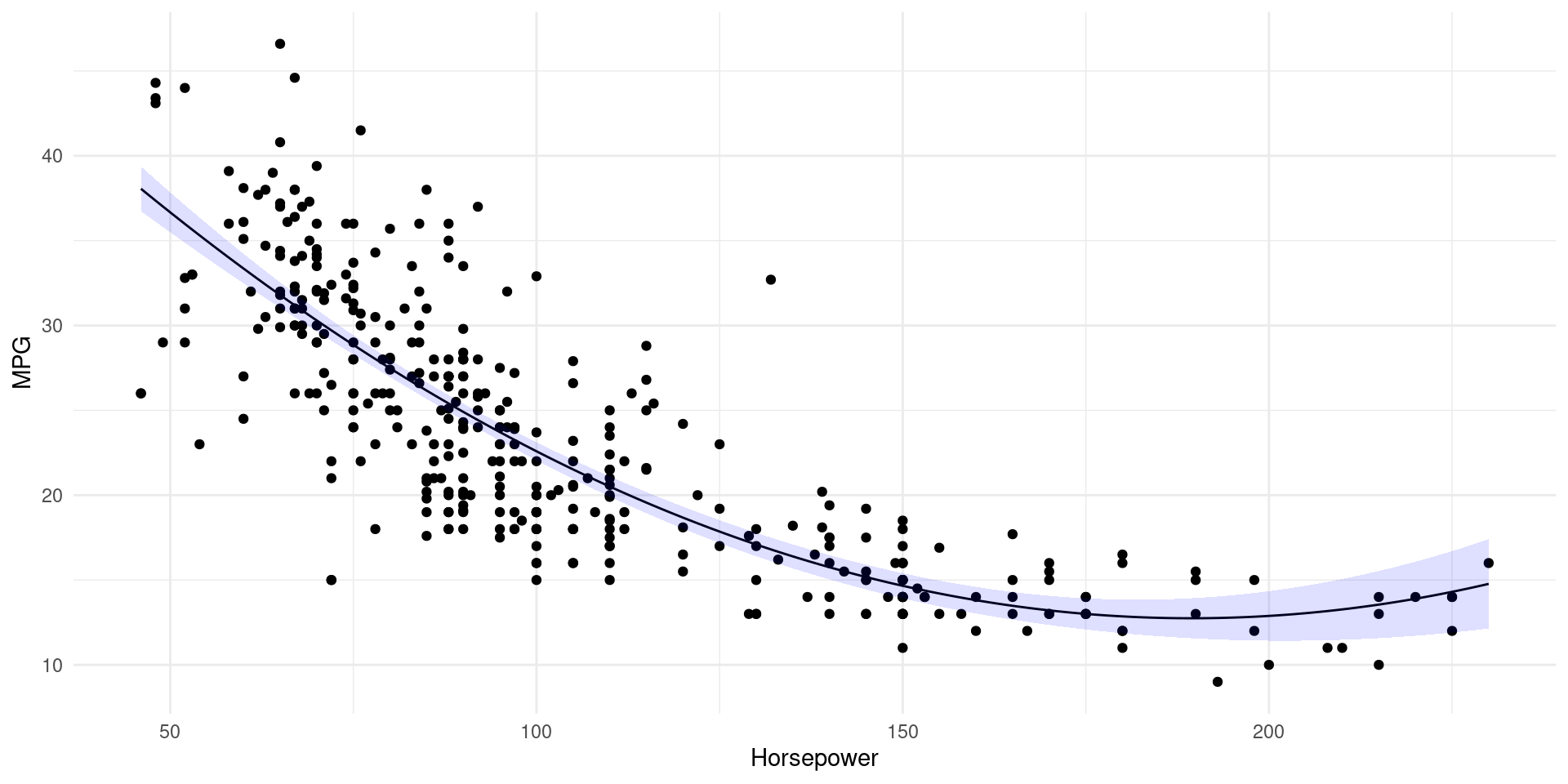
Regression analysis in real life

Following current trends, the next PM will be in office for approximately minus 200 days pic.twitter.com/avLQE9i1yy
— Rob Sansom (@Sansom_Rob) October 20, 2022

The limits of classic regression models

Linear and logistic regression are a good first shot for building ML models

Easy-to-interpret coefficients
Intuitive (ish) ways to assess variable importance
Often good out-of-the-box predictions

However…

Assumption that the predictors are linearly related to the outcome is restrictive
We have seen, for instance, that accounting for higher order polynomial relationships can produce better model fit

Example

Think of the relationship between lstat and medv in Boston (💻 Week 05 Lab)

Enter non-linear methods

These algorithms do not make (strong) statistical assumptions about the data
The focus is more on predictive rather than explanatory power

The Decision Tree

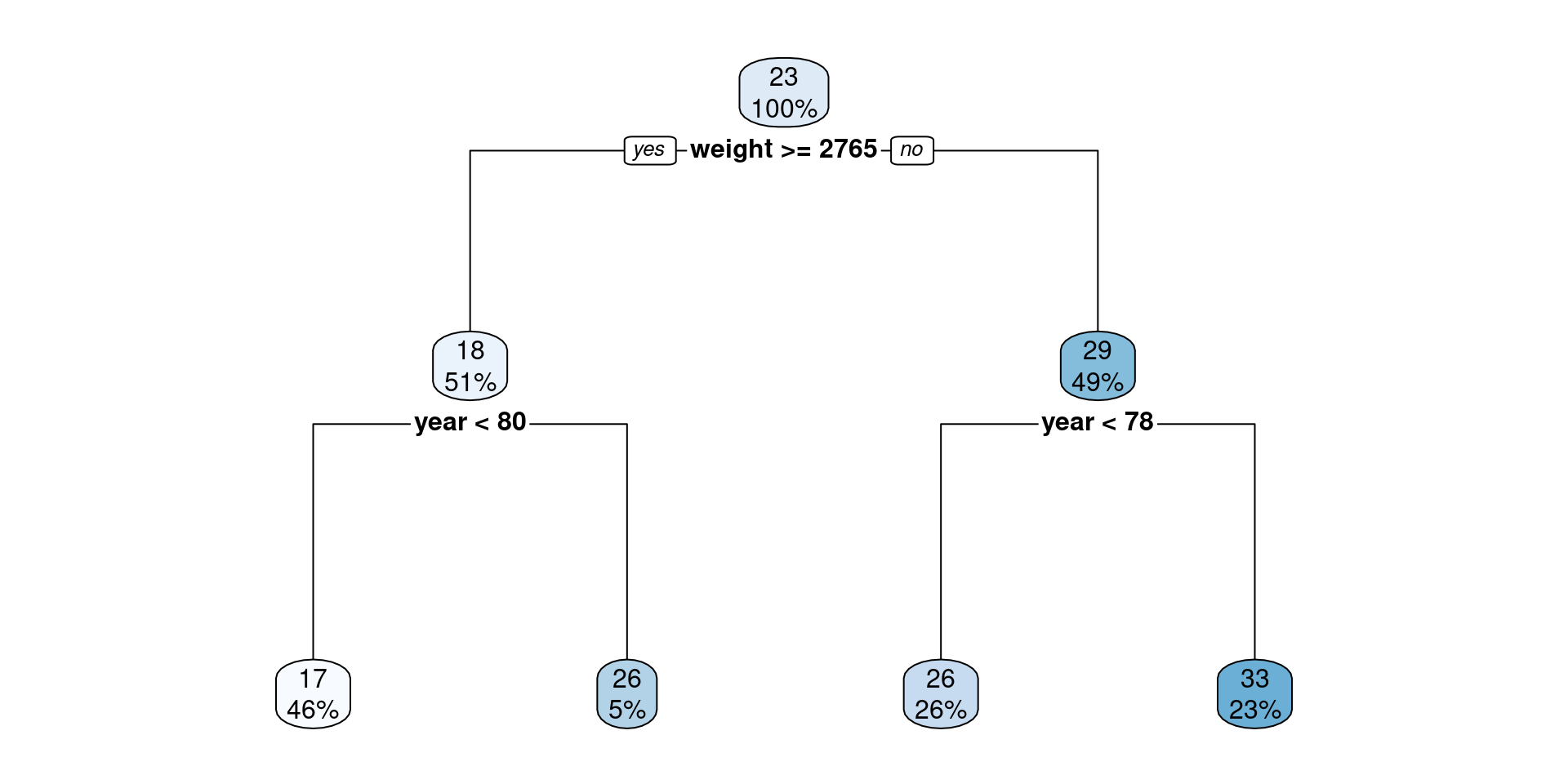
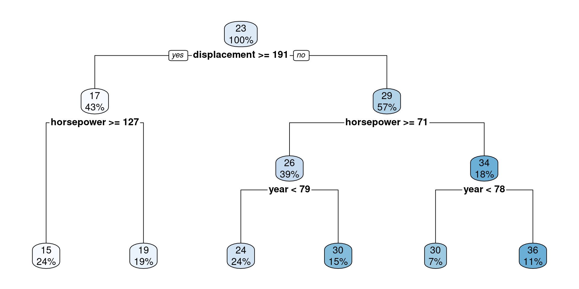
Decision Tree for a Regression task

Using the Auto dataset, predict mpg with a tree-based model using weight and year as features.

Source Code

Tip

Use the code below to replicate the plot from the previous slide.
Found a bug? Report it on Slack.
💡 Check out this tutorial of rpart.plot.

library(ISLR2)      # to load Boston data
library(tidyverse)  # to use things like the pipe (%>%), mutate and if_else

library(rpart)      # a library that contains decision tree models
library(rpart.plot) # a library that plots rpart models 

# The function rpart below fits a decision tree to the data
# You can control various aspects of the rpart fit with the parameter `control`
# Type ?rpart.control in the R console to see what else you can change in the algorithm

tree.reg <- rpart(mpg ~ weight + year, data = Auto, control = list(maxdepth = 2))

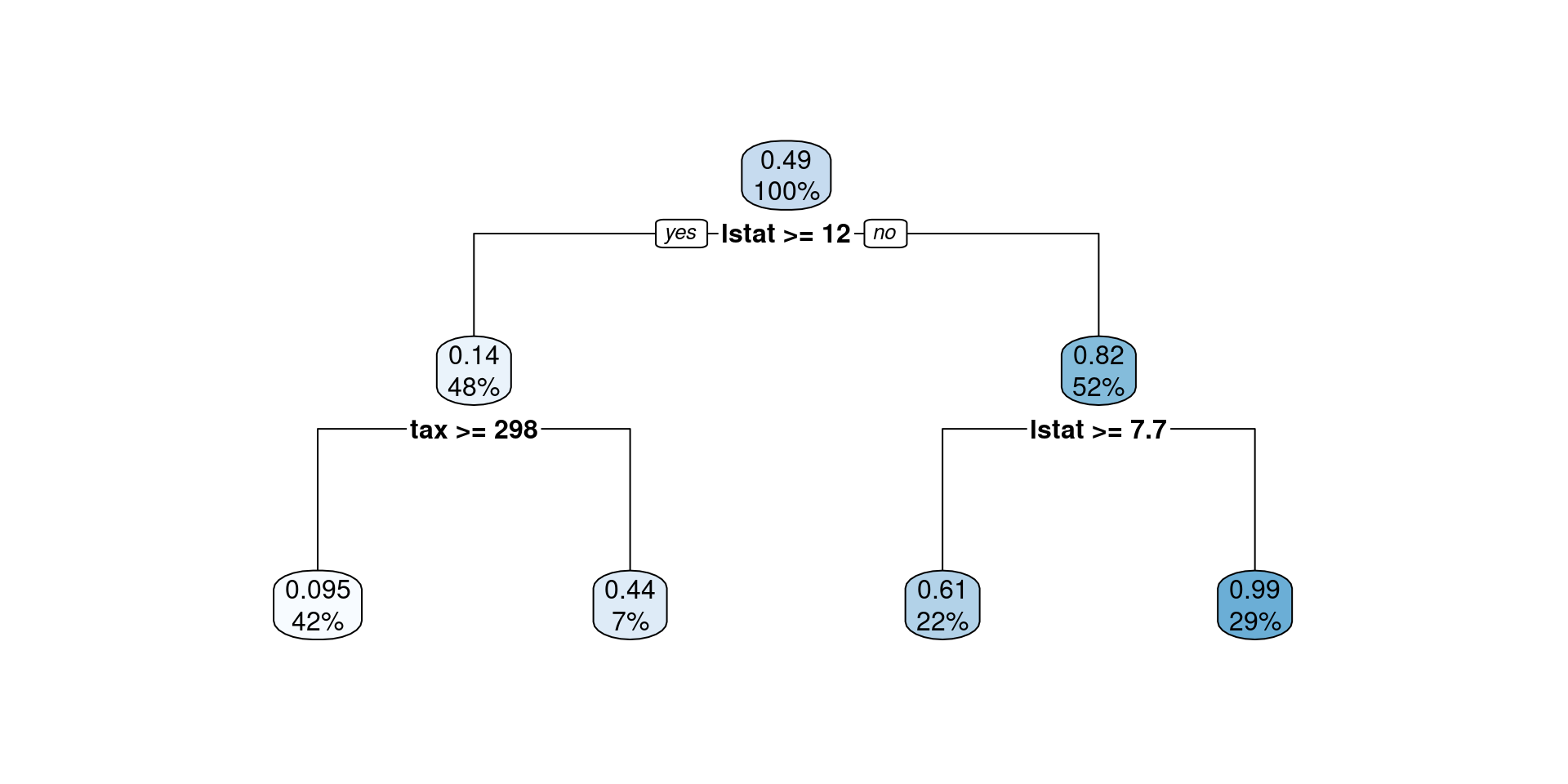
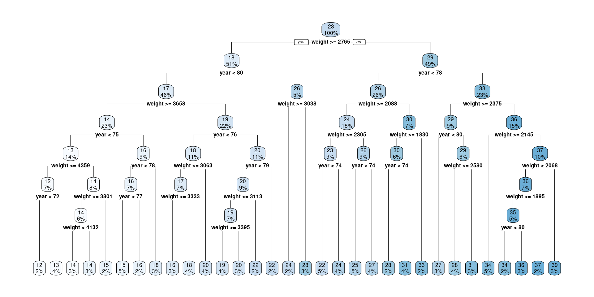
rpart.plot(tree.reg)

Decision Tree for a Classification task

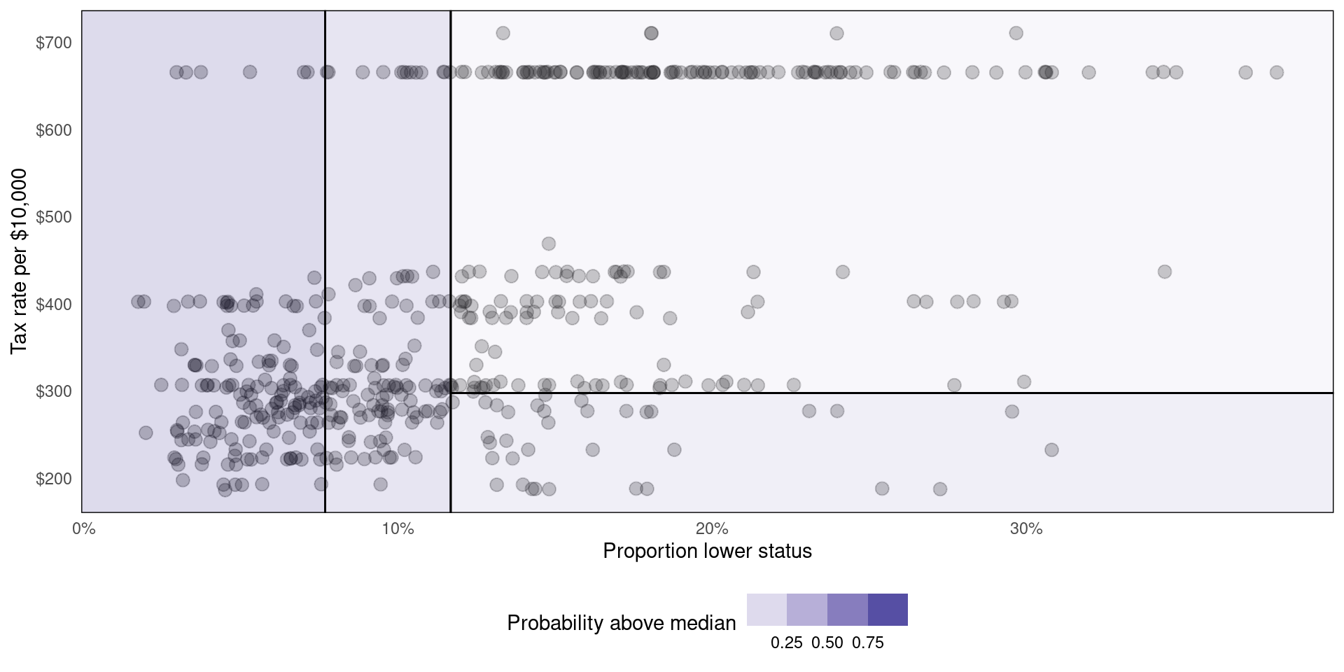
Using the Boston dataset, predict whether medv is above the median using crim and tax:

Source Code

Tip

Use the code below to replicate the plot from the previous slide.
Found a bug? Report it on Slack.
💡 Check out this tutorial of rpart.plot.

library(ISLR2)      # to load Boston data
library(tidyverse)  # to use things like the pipe (%>%), mutate and if_else

library(rpart)      # a library that contains decision tree models
library(rpart.plot) # a library that plots rpart models 

# Add a column named `medv_gtmed` to indicate whether tax rate is above median
Boston <- Boston %>% mutate(medv_gtmed = if_else(medv > median(medv), TRUE, FALSE))

# The function rpart below fits a decision tree to the data
# You can control various aspects of the rpart fit with the parameter `control`
# Type ?rpart.control in the R console to see what else you can change in the algorithm

tree.class <- rpart(medv_gtmed ~ lstat + tax, data = Boston, control = list(maxdepth = 2))

rpart.plot(tree.class)

How does it work?

What’s going on behind the scenes?

How decision trees work:

Divide the predictor space into \(\mathbf{J}\) distinct regions \(R_1\), \(R_2\),…,\(R_j\).
Take the mean of the response values in each region

Here’s how the regions were created in our regression/classification examples ⏭️

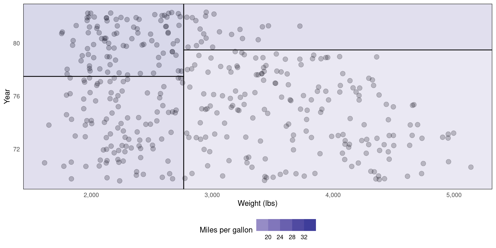
Alternative representation of decision tree (Regression)

Alternative representation of decision tree (Classification)

Source code

Tip

Use the code in the following slides to replicate the plot from those two plots.
Found a bug? Report it on Slack.
💡Check out the parttree documentation for how to customize your plot
💡Learn more about data visualisation with ggplot2 on R for Data Science - Chapter 3

Source Code (regression)

First, you will have to install the parttree package:

# Follow the instructions by the developers of the package
# (https://github.com/grantmcdermott/parttree)

install.packages("remotes")
remotes::install_github("grantmcdermott/parttree", force = TRUE)

Then:

library(ISLR2)      # to load Boston data
library(tidyverse)  # to use things like the pipe (%>%), mutate and if_else

library(rpart)      # a library that contains decision tree models
library(parttree)   # R package for plotting simple decision tree partitions

# The function rpart below fits a decision tree to the data
# You can control various aspects of the rpart fit with the parameter `control`
# Type ?rpart.control in the R console to see what else you can change in the algorithm

tree.reg <- rpart(mpg ~ weight + year, data = Auto, control = list(maxdepth = 2))

Auto %>%
   ggplot(aes(x = weight, y = year)) +
   geom_jitter(size = 3, alpha = 0.25) +
   geom_parttree(data = tree.reg, aes(fill = mpg), alpha = 0.2) +
   theme_minimal() +
   theme(panel.grid = element_blank(), legend.position = 'bottom') +
   scale_x_continuous(labels = scales::comma) +
   scale_fill_steps2() +
   labs(x = 'Weight (lbs)', y = 'Year', fill = 'Miles per gallon')

Source Code (classification)

First, you will have to install the parttree package:

# Follow the instructions by the developers of the package
# (https://github.com/grantmcdermott/parttree)

install.packages("remotes")
remotes::install_github("grantmcdermott/parttree", force = TRUE)

Then:

library(ISLR2)      # to load Boston data
library(tidyverse)  # to use things like the pipe (%>%), mutate and if_else

library(rpart)      # a library that contains decision tree models
library(parttree)   # R package for plotting simple decision tree partitions

# Add a column named `medv_gtmed` to indicate whether tax rate is above median
Boston <- Boston %>% mutate(medv_gtmed = if_else(medv > median(medv), TRUE, FALSE))

# The function rpart below fits a decision tree to the data
# You can control various aspects of the rpart fit with the parameter `control`
# Type ?rpart.control in the R console to see what else you can change in the algorithm

tree.class <- rpart(medv_gtmed ~ lstat + tax, data = Boston, control = list(maxdepth = 2))

Boston %>%
   ggplot(aes(x = lstat, y = tax)) +
   geom_jitter(size = 3, alpha = 0.25) +
   geom_parttree(data = tree.class, aes(fill = medv_gtmed), alpha = 0.2) +
   theme_minimal() +
   theme(panel.grid = element_blank(), legend.position = 'bottom') +
   scale_x_continuous(labels = scales::percent_format(scale = 1)) +
   scale_y_continuous(labels = dollar) +
   scale_fill_steps2() +
   labs(x = 'Proportion lower status', y = 'Tax rate per $10,000', fill = 'Probability above median')

How are regions created?

Recursive binary splitting

Top down

Start from the top of the tree
Then perform splits at a current level of depth

Greedy

Splits are “local” not global
Only cares about data in the current branch

For regression…

The tree selects a predictor \(X_j\) and a cutpoint \(s\) that minimises the residual sum of squares.

We define two half planes \(R_1(j,s) = \left\{X|X_j < s\right\}\) and \(R_2(j,s) = \left\{X|X_j \geq s\right\}\) and find \(j\) and \(s\) by minimising.

\[ \sum_{i: x_i \in R_1(j,s)} (y_i - \hat{y}_{R_1})^2 + \sum_{i: x_i \in R_2(j,s)} (y_i - \hat{y}_{R_2})^2 \]

For classification…

The tree selects a predictor \(X_j\) and a cutpoint \(s\) that maximises node purity.
Gini index: \(G = \sum_{k = 1}^{K} \hat{p}_{mk}(1 - \hat{p}_{mk})\)
Entropy: \(D = - \sum_{k = 1}^{K} \hat{p}_{mk}\log \hat{p}_{mk}\)

What can go wrong

When trees run amock

Trees can become too complex if we are not careful
It can lead to something called overfitting
- High training set predictive power
- Low test set predictive power
Let’s see one example ⏭️

The following tree is TOO specialised

Partition visualisation of the same tree

How to fix it

Pruning the tree

Hyperparameters are model-specific dials that we can tune
- Things like max tree depth, or min samples per leaf
As with model selection, there is no one one-size-fits-all approach to hyperparameter tuning.
Instead, we experiment with resampling
- Most frequently, k-fold cross-validation

k-fold cross-validation

We experimented with k-fold CV in 🗓️ Week 04’s lecture/workshop
We will revisit this topic in 🗓️ Week 07’s lab
Not compulsory for ✍️ Summmative Problem Set (01) | W05-W07

Cost Complexity

We apply \(\alpha\) which is a non-negative value to prune the tree.
For example, when \(\alpha = 0.02\) we can create a less complex tree.

What’s Next

After our 10-min break ☕:

Support Vector Machine
Tips for the Summative Problem Set 01

🗓️ Week 05: Decision Trees

Regression analysis in real life

The limits of classic regression models

The limits of classic regression models

However…

Example

Enter non-linear methods

The Decision Tree

Decision Tree for a Regression task

Source Code

Decision Tree for a Classification task

Source Code

How does it work?

What’s going on behind the scenes?

Alternative representation of decision tree (Regression)

Alternative representation of decision tree (Classification)

Source code

Source Code (regression)

Source Code (classification)

How are regions created?

Top down

Greedy

For regression…

For classification…

What can go wrong

When trees run amock

The following tree is TOO specialised

Partition visualisation of the same tree

How to fix it

Pruning the tree

Cost Complexity

What’s Next

🗓️ Week 05:
Decision Trees