🗓️ Week 03
Classifiers - Part I

DS202 Data Science for Social Scientists

Dr. Jon Cardoso-Silva

@LSEDataScience

10/14/22

What we will cover today

• Regression vs Classification
• Logistic Regression
• Interpreting coefficients
• Multiple
  Logistic
  Regression
• What’s Next

Regression vs Classification

Classification

• We have so far only modelled quantitative responses.
• Today, we focus on predicting categorical, or qualitative, responses.

The generic supervised model:

\[ Y = \operatorname{f}(X) + \epsilon \]

still applies, only this time \(Y\) is categorical. ➡️

Our categorical variables of interest take values in an unordered set \(\mathcal{C}\), such as:

• \(\text{eye color} \in \mathcal{C} = \{\color{brown}{brown},\color{blue}{blue},\color{green}{green}\}\)
• \(\text{email} \in \mathcal{C} = \{spam, ham\}\)
• \(\text{football results} \in \mathcal{C} \{away\ win,draw,home\ win\}\)

Opening slides - Unordered here is an important distinction. - We can also call it a class

Why can’t I use linear regression?

What if I just coded each category as a number?

\[ Y = \begin{cases} 1 &\text{if}~\color{brown}{brown},\\ 2 &\text{if}~\color{blue}{blue},\\ 3 &\text{if}~\color{green}{green}. \end{cases} \]

What could go wrong?

How would you interpret a particular prediction if your model returned:

• \(\hat{y} = ~~1.5\) or
• \(\hat{y} = ~~0.1\) or
• \(\hat{y} = 20.0\)?

Key takeaway: Regression is not suitable for all problems. - regression cannot accommodate a qualitative response with more than two classes - regression will not provide meaningful estaimtes of Pr(Y|X)

More on Classification

• Often we are more interested in estimating the probabilities that \(X\) belongs to each category in \(\mathcal{C}\).

• For example, it is sometimes more valuable to have an estimate of the probability that an insurance claim is fraudulent, than a classification fraudulent or not.

• A successful gambling strategy, for instance, requires placing bets on outcomes to which you believe the bookmakers have assigned incorrect probabilities. Knowing the most likely outcome is not enough!

Note

Statistical models for ordinal response, when sets are discrete but have an order, are outside the scope of this course. Should you need to create models for ordinal variables, consult “ordinal logistic regression”. A good reference about this is (Agresti 2019, chap. 6).

Key takeaway: normally, we estimate

Speaking of Probabilities…

Let’s talk about three possible interpretations of probability:

Classical

Frequentist

Bayesian

Events of the same kind can be reduced to a certain number of equally possible cases.

Example: coin tosses lead to either heads or tails \(1/2\) of the time ( \(50\%/50\%\))

What would be the outcome if I repeat the process many times?

Example: if I toss a coin \(1,000,000\) times, I expect \(\approx 50\%\) heads and \(\approx 50\%\) tails outcome.

What is your judgement of the likelihood of the outcome? Based on previous information.

Example: if I know that this coin has symmetric weight, I expect a \(50\%/50\%\) outcome.

Source: (DeGroot and Schervish 2003)

Speaking of Probabilities…

For our purposes:

• Probabilities are numbers between 0 and 1
• The sum of all possible outcomes of an event must sum to 1.
• It is useful to think of things as probabilities

Note

💡 Although there is no such thing as “a probability of \(120\%\)” or “a probability of \(-23\%\)”, you could still use this language to refer to increase or decrease in an outcome.

Logistic Regression

The Logistic Regression model

Consider a binary response:

\[ Y = \begin{cases} 0 \\ 1 \end{cases} \]

We model the probability that \(Y = 1\) using the logistic function (aka. sigmoid curve):

\[ Pr(Y = 1|X) = p(X) = \frac{e^{\beta_0 + \beta_1X}}{1 + e^{\beta_0 + \beta_1 X}} \]

• This is how this function looks like

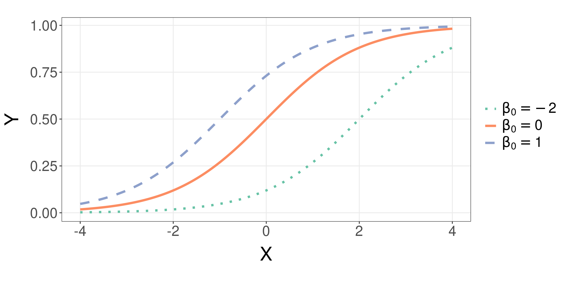
The Logistic function

• Changing \(\beta_0\) while keeping \(\beta_1 = 1\):

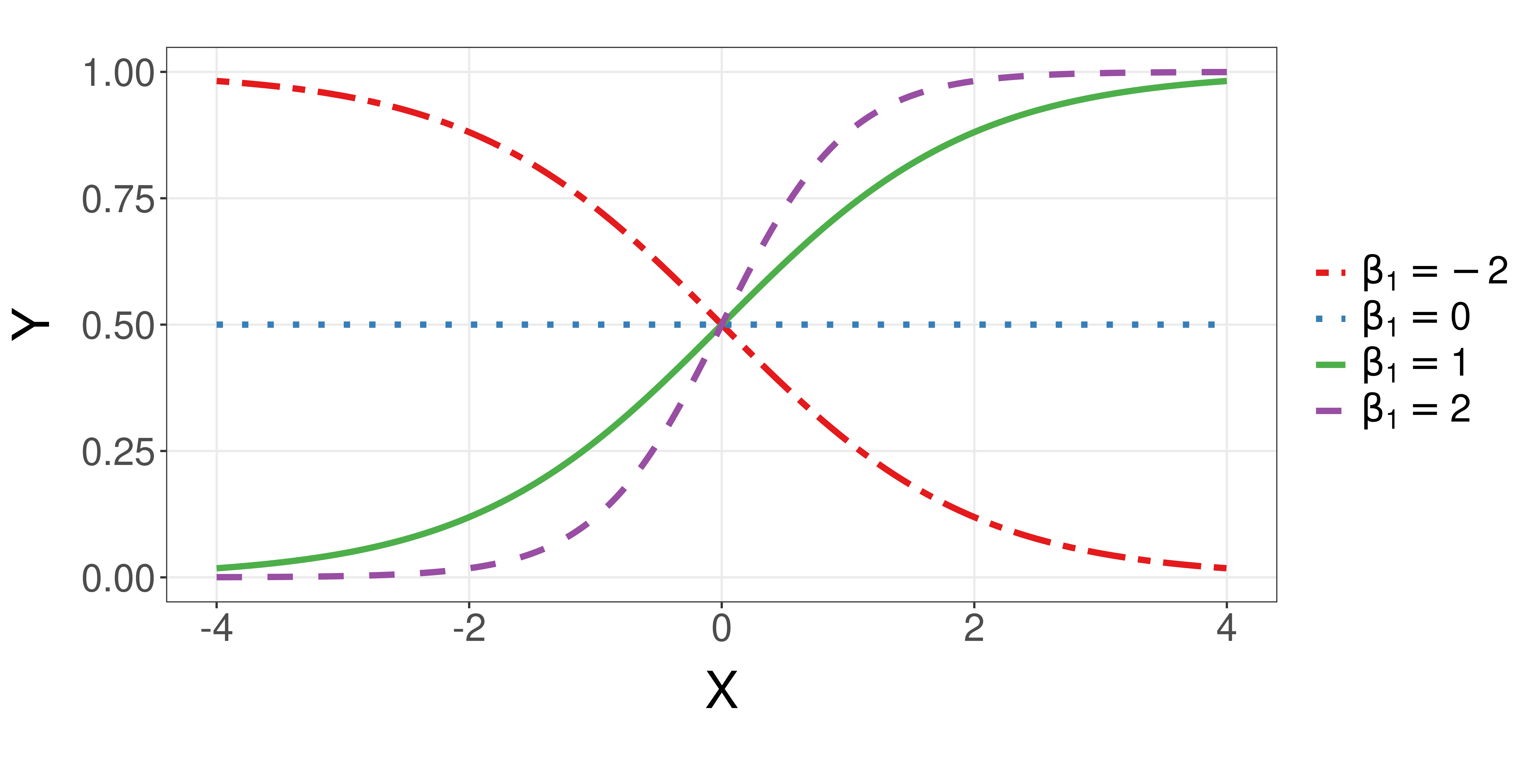
The Logistic function (cont.)

• Keep \(\beta_0 = 0\) but vary \(\beta_1\):

Maximum likelihood estimate

As with linear regression, the coefficients are unknown and need to be estimated from training data:

\[ \hat{p}(X) = \frac{e^{\hat{\beta}_0 + \hat{\beta}_1X}}{1 + e^{\hat{\beta}_0 + \hat{\beta}_1 X}} \]

We estimate these by maximising the likelihood function:

\[ \max \ell(\beta_0, \beta_1) = \prod_{i:y_i=1}{p(x_i)} \prod_{i':y_{i'}=0} (1 - p(x_{i'})), \]

and we call this method the Maximum Likelihood Estimate (MLE).

➡️ As usual, there are multiple ways to solve this equation!

Key takeaway of this slide: MLE (logistic regression) is analogous to OLS (linear regression).

Intuition: What are the values for \(\alpha\) and \(\beta\) that generate predicted probabilities, \(\hat{Y}_i\) for each training observation that are as close as possible to the realised outcomes, \(Y_i\)?

💡 If you want to read on how exactly this is solved check this link

Solutions to MLE

• MLE is much more difficult to solve than the least squares formulations.
• Most solutions rely on a variant of the Hill Climbing algorithm

How do you find the latitude and longitude of a mountain peak if you can’t see very far?

• Start somewhere.
• Look around for the best way to go up.
• Go a small distance in that direction.
• Look around for the best way to go up.
• Go a small distance in that direction.
• \(\cdots\)

Interpreting coefficients

Since we now mostly care about probabilities, how do the odds change according to features of the customers?

The concept of odds

The quantity below is called the odds:

\[ \frac{p(X)}{1 - p(X)} = e^{\beta_0 + \beta_1 X} \]

Example

If the odds are 9, then \(\frac{p(X)}{(1-p(X))} = 9 \Rightarrow p(X) = 0.9\).

This means that 9 out of 10 people will default.

Tip

How to interpret \(\beta_1\)

If X increases one unit then the odds increase by a factor of \(e^{\beta_1}\)

Log odds or logit

• It is also useful to think of the odds in log terms.

\[ log\left(\frac{p(X)}{1 - p(X)}\right) = \beta_0 + \beta_1 X \]

• We call the quantity above the log odds or logit

Tip

How to interpret \(\beta_1\)

If X increases one unit then the log odds increase by \(\beta_1\)

Example: Default data

A sample of the data:

library(ISLR2)

head(ISLR2::Default, n=15)

   default student   balance    income
1       No      No  729.5265 44361.625
2       No     Yes  817.1804 12106.135
3       No      No 1073.5492 31767.139
4       No      No  529.2506 35704.494
5       No      No  785.6559 38463.496
6       No     Yes  919.5885  7491.559
7       No      No  825.5133 24905.227
8       No     Yes  808.6675 17600.451
9       No      No 1161.0579 37468.529
10      No      No    0.0000 29275.268
11      No     Yes    0.0000 21871.073
12      No     Yes 1220.5838 13268.562
13      No      No  237.0451 28251.695
14      No      No  606.7423 44994.556
15      No      No 1112.9684 23810.174

How the data is spread:

summary(ISLR2::Default$default)

  No  Yes 
9667  333 

summary(ISLR2::Default$balance)

   Min. 1st Qu.  Median    Mean 3rd Qu.    Max. 
    0.0   481.7   823.6   835.4  1166.3  2654.3 

summary(ISLR2::Default$income)

   Min. 1st Qu.  Median    Mean 3rd Qu.    Max. 
    772   21340   34553   33517   43808   73554 

summary(ISLR2::Default$student)

  No  Yes 
7056 2944 

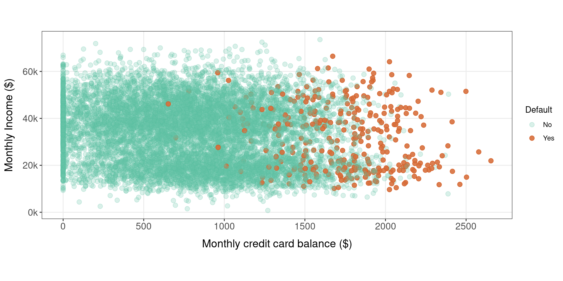
Who is more likely to default?

• You can see that large balance leads more easily to default

This is essentially the same plot as Figure 4.1 in (James et al. 2021)

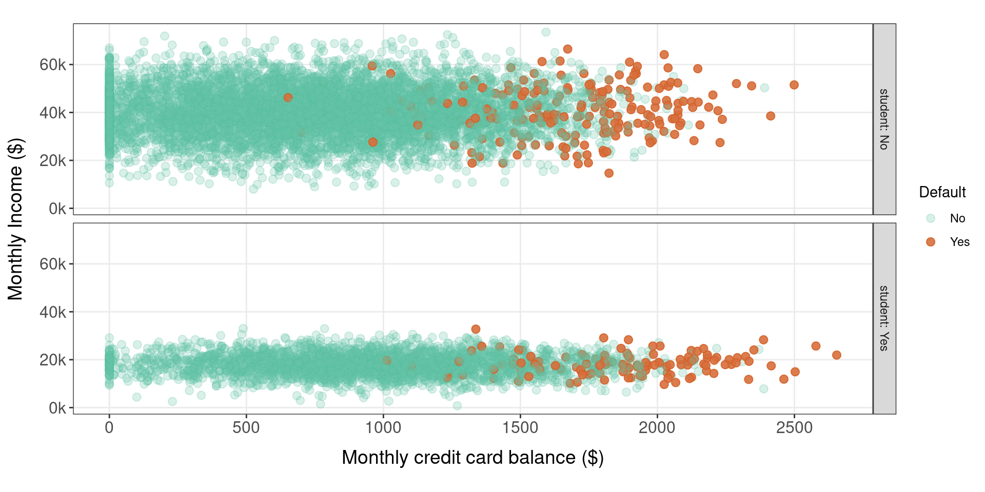
Does it matter if customer is a student?

Simple logistic regression models

• Income 💰

income_model <- 
  glm(default ~ income, data=ISLR2::Default, family=binomial)
cat(sprintf("beta_0 = %.5f | beta_1 = %e",
            income_model$coefficients["(Intercept)"],
            income_model$coefficients["income"]))

beta_0 = -3.09415 | beta_1 = -8.352575e-06

• Balance 💸

balance_model <- 
  glm(default ~ balance, data=ISLR2::Default, family=binomial)
cat(sprintf("beta_0 = %.5f | beta_1 = %.4f",
            balance_model$coefficients["(Intercept)"],
            balance_model$coefficients["balance"]))

beta_0 = -10.65133 | beta_1 = 0.0055

• Student 🧑‍🎓

student_model <- 
  glm(default ~ student, data=ISLR2::Default, family=binomial)
cat(sprintf("beta_0 = %.5f | beta_1 = %.4f",
            student_model$coefficients["(Intercept)"],
            student_model$coefficients["studentYes"]))

beta_0 = -3.50413 | beta_1 = 0.4049

Note

Logistic regression coefficients are a bit trickier to interpret when compared to those of linear regression. Let’s look at how it works ➡️

• Gather answers from students.

Example: Default vs Balance

• Model: Default vs Balance 💸

\[ \hat{y} = \frac{e^{-10.65133 + 0.005498917X}}{1 + e^{-10.65133 + 0.005498917X}} \]

That is:

\[ \begin{align} \hat{\beta}_0 &= -10.65133\\ \hat{\beta}_1 &= 0.005498917 \end{align} \]

Interpreting \(\hat{\beta}_0\):

• In the absence of balance information:
  • Log odds: \(-10.65133\)
  • Odds : \(e^{-10.65133} = 2.366933 \times 10^{-5}\) \[ \begin{align} p(\text{default}=\text{Yes}) &= \frac{\text{odds}}{(1 + \text{odds})} \\ &= 2.366877 \times 10^{-5}\end{align} \]

Interpreting \(\hat{\beta}_1\):

• With balance information:
  • Log odds: \(0.005498917\)
  • Odds : \(e^{0.005498917} = 1.005514\)
  • That is, for every \(\$1\) increase in balance, the probability of default increases

• Note that the increase is cumulative, not linear. It depends on where X is.

Example: Default vs Income

• Model: Default vs Income 💰

\[ \hat{y} = \frac{e^{-3.094149 - 8.352575 \times 10^{-6} X}}{1 + e^{-3.094149 - 8.352575 \times 10^{-6} X}} \]

That is:

\[ \begin{align} \hat{\beta}_0 &= - 3.094149\\ \hat{\beta}_1 &= - 8.352575 \times 10^{-6} \end{align} \]

Interpreting \(\hat{\beta}_0\):

• In the absence of balance information:
  • Log odds: \(- 3.094149\)
  • Odds : \(e^{- 3.094149} = 0.04531355\) \[ \begin{align} p(\text{default}=\text{Yes}) &= \frac{\text{odds}}{(1 + \text{odds})} \\ &= 0.04334924 = 4.33\%\end{align} \]

Interpreting \(\hat{\beta}_1\):

• With balance information:
  • Log odds: \(- 8.352575\)
  • Odds : \(e^{- 8.352575} = 0.9999916\)
  • That is, for every \(\$1\) increase in income, the probability of default decreases

• Note that the increase is cumulative, not linear. It depends on where X is.

Example: Default vs Is Student?

• Model: Default vs Student 🧑‍🎓

\[ \hat{y} = \frac{e^{-3.504128 + 0.4048871 X}}{1 + e^{-3.504128 + 0.4048871 X}} \]

That is:

\[ \begin{align} \hat{\beta}_0 &= -3.504128\\ \hat{\beta}_1 &= +0.4048871 \end{align} \]

Interpreting \(\hat{\beta}_0\):

• In the absence of balance information:
  • Log odds: \(-3.504128\)
  • Odds : \(e^{- 3.504128} = 0.03007299\) \[ \begin{align} p(\text{default}=\text{Yes}) &= \frac{\text{odds}}{(1 + \text{odds})} \\ &= 0.02919501 \approx 2.92\%\end{align} \]

Interpreting \(\hat{\beta}_1\):

• With balance information:
  • Log odds: \(0.4048871\)
  • Odds : \(e^{0.4048871} = 1.499133\)
• If person is a student, then the probability of default increases

Model info

The output of summary is similar to that of linear regression:

• Model: Default vs Balance 💸

summary(balance_model)

Call:
glm(formula = default ~ balance, family = binomial, data = ISLR2::Default)

Deviance Residuals: 
    Min       1Q   Median       3Q      Max  
-2.2697  -0.1465  -0.0589  -0.0221   3.7589  

Coefficients:
              Estimate Std. Error z value Pr(>|z|)    
(Intercept) -1.065e+01  3.612e-01  -29.49   <2e-16 ***
balance      5.499e-03  2.204e-04   24.95   <2e-16 ***
---
Signif. codes:  0 '***' 0.001 '**' 0.01 '*' 0.05 '.' 0.1 ' ' 1

(Dispersion parameter for binomial family taken to be 1)

    Null deviance: 2920.6  on 9999  degrees of freedom
Residual deviance: 1596.5  on 9998  degrees of freedom
AIC: 1600.5

Number of Fisher Scoring iterations: 8

Confidence Intervals

confint(balance_model)

                    2.5 %       97.5 %
(Intercept) -11.383288936 -9.966565064
balance       0.005078926  0.005943365

Wraping up on coefficients:

• Pay attention to the sign of the coefficient. The sign of the coefficients indicate the direction of the association.
• If the value of a predictor increases, we look at the sign of its coefficient:
  • If it is a ➕ positive coefficient, we predict an increase in the probability of the class
  • If it is a ➖ negative coefficient, we predict a decrease in the probability of the class

Multiple
Logistic
Regression

Multiple Logistic Regression

• It is straightforward to extend the logistic model to include multiple predictors:

\[ log \left( \frac{p(X)}{1-p(X)} \right)=\beta_0 + \beta_1 X_1 + \ldots + \beta_p X_p \]

\[ p(X) = \frac{e^{\beta_0 + \beta_1 X_1 + \ldots + \beta_p X_p}}{1 + e^{\beta_0 + \beta_1 X_1 + \ldots + \beta_p X_p}} \]

• Most things are still available (hypothesis test, confidence intervals, etc.)
• Let’s explore the output and summary of the full model ⏭️

Fitting all predictors of Default

Full Model

full_model <- glm(default ~ ., data=ISLR2::Default, family=binomial)
summary(full_model)

Call:
glm(formula = default ~ ., family = binomial, data = ISLR2::Default)

Deviance Residuals: 
    Min       1Q   Median       3Q      Max  
-2.4691  -0.1418  -0.0557  -0.0203   3.7383  

Coefficients:
              Estimate Std. Error z value Pr(>|z|)    
(Intercept) -1.087e+01  4.923e-01 -22.080  < 2e-16 ***
studentYes  -6.468e-01  2.363e-01  -2.738  0.00619 ** 
balance      5.737e-03  2.319e-04  24.738  < 2e-16 ***
income       3.033e-06  8.203e-06   0.370  0.71152    
---
Signif. codes:  0 '***' 0.001 '**' 0.01 '*' 0.05 '.' 0.1 ' ' 1

(Dispersion parameter for binomial family taken to be 1)

    Null deviance: 2920.6  on 9999  degrees of freedom
Residual deviance: 1571.5  on 9996  degrees of freedom
AIC: 1579.5

Number of Fisher Scoring iterations: 8

Confidence Intervals

confint(full_model)

                    2.5 %        97.5 %
(Intercept) -1.185902e+01 -9.928174e+00
studentYes  -1.109018e+00 -1.822147e-01
balance      5.294898e-03  6.204587e-03
income      -1.304712e-05  1.912447e-05

What’s Next

After our 10-min break ☕:

• Bayes’ Theorem
• The Naive Bayes algorithm
• Thresholds
• Confusion Matrix
• ROC Curve
• What will happen in our 💻 labs this week?

References

Agresti, Alan. 2019. An Introduction to Categorical Data Analysis. Third edition. Wiley Series in Probability and Statistics. Hoboken, NJ: John Wiley & Sons.

DeGroot, Morris H., and Mark J. Schervish. 2003. Probability and Statistics. 3. ed., international edition. Boston Munich: Addison-Wesley.

James, Gareth, Daniela Witten, Trevor Hastie, and Robert Tibshirani. 2021. An Introduction to Statistical Learning: With Applications in R. Second edition. Springer Texts in Statistics. New York NY: Springer. https://www.statlearning.com/.