🗓️ Week 01
Overview of core concepts

DS202 Data Science for Social Scientists

Dr. Jon Cardoso-Silva

@LSEDataScience

9/30/22

What we will cover today

• What do we mean by data science?
• The
  Data
  Science
  Workflow
• How is that different to what I have learned in my previous stats courses?
• Machine Learning
• Training algorithm
• What’s Next?
• Thank you

What do we mean by data science?

Data science is…

“[…] a field of study and practice that involves the collection, storage, and processing of data in order to derive important 💡 insights into a problem or a phenomenon.

Such data may be generated by humans (surveys, logs, etc.) or machines (weather data, road vision, etc.),

and could be in different formats (text, audio, video, augmented or virtual reality, etc.).”

(Shah 2020, chap. 1) - Emphasis and emojis are of my own making.

The mythical unicorn 🦄

knows everything about statistics

able to communicate insights perfectly

fully understands businesses like no one

is a fluent computer programmer

Of course, such a person does not exist!

See (Davenport 2020) for a more in-depth discussion about this

In reality…

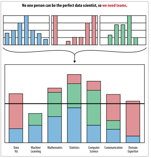
We are all jugglers 🤹

• Everyone brings a different skill set.
• We need multi-disciplinary teams.
• Good data scientists know a bit of everything.
  • Not fluent in all things
  • Understands their strenghts and weaknessess
  • They know when and where to interface with others

See (Schutt and O’Neil 2013, chap. 1) for more on this.

The
Data
Science
Workflow

The Data Science Workflow

⚠️ Note that this is a simplified version of what happens in a data science project.
In practice, the process is not linear and there are many feedback loops.

The Data Science Workflow

It is often said that 80% of the time and effort spent on a data science project goes to the tasks highlighted above.

The Data Science Workflow

This course is about Machine Learning. So, in most examples and tutorials, we will assume that we already have good quality data.

How is that different to what I have learned in my previous stats courses?

Data Science and Social Science

In reality, data scientists work as a multidisciplinary group, collaborating towards a common goal.

Content borrowed from ME314 Day 1

• Social science: The goal is typically explanation
• Data science: The goal is frequently prediction, or data exploration
• Many of the same methods are used for both objectives

Check (Shmueli 2010) for a discussion about this topic.

Machine Learning

What does it mean to learn something?

Predicting a sequence intuitively

• Say our data is the following simple sequence: \(6, 9, 12, 15, 18, 21, 24, ...\)
• What number do you expect to come next? Why?
• It is very likely that you guessed that
  \(\operatorname{next number}=27\)
• We spot that the sequence follows a pattern
• From this, we notice — we learn — that the sequence is governed by:
  \(\operatorname{next number} = \operatorname{previous number} + 3\)

Predicting a sequence (formula)

The next number is a function of the previous one:

\[ \operatorname{next number} = f(\operatorname{previous number}) \]

Predicting a sequence (generic formula)

In general terms, we can represented it as:

\[ \operatorname{Y} = f(\operatorname{X}) \]

where:

• \(Y\): a quantitative response.
  It goes by many names: dependent variable, response, target, outcome
• \(X\): a set of predictors,
  also called inputs, regressors, covariates, features, independent variables.
• \(f\): the systematic information that \(X\) provides about \(Y\)

Predicting a sequence (generic formula)

In general terms, we can represented it as:

\[ \operatorname{Y} = f(\operatorname{X}) + \epsilon \]

where:

• \(Y\): the output
• \(X\): a set of inputs
• \(f\): the systematic information that \(X\) provides about \(Y\)
• \(\epsilon~~\): a random error term

In reality, there is some error \(\epsilon\) that cannot be reduced.

Approximating \(f\)

• \(f\) is almost always unknown
• We aim to find an approximation (a model). Let’s call it \(\hat{f}\)
• that can then use it to predict values of \(Y\) for whatever \(X\).
• That is: \(\hat{Y} = \hat{f}(X)\)

What is Machine Learning?

• Statistical learning, or Machine learning, refers to a set of approaches for estimating \(f\).
• Each algorithm you will learn on this course has its own way to determine \(\hat{f}\) given data

Types of learning

In general terms, there are two main ways to learn from data:

Supervised Learning

• Each observation (\(x_i\)) has an outcome associated with it (\(y_i\)).
• Your goal is to find a \(\hat{f}\) that produces \(\hat{Y}\) value close to the true \(Y\) values.
• Our focus on 🗓️ Weeks 2, 3, 4 & 5.

Unsupervised Learning

• You have observations (\(x_i\)) but there is no response variable.
• Your goal is to find a \(\hat{f}\), focused only on \(X\) that best represents the patterns in the data.
• Our focus on 🗓️ Weeks 7 & 8.

Training algorithm

Now let’s shift our attention to understanding:

• how we structure our data for supervised learning
• the different sources of statistical errors

Data Structure

Let’s go back to our example:

Our simple sequence:

\(6, 9, 12, 15, 18, 21, 24\)

Becomes:

\(X\)	\(Y\)
6	9
9	12
12	15
15	18
18	21
21	24

And for prediction:

\(X\)	\(\hat{Y}\)
24	?

we present the \(X\) values and ask the fitted model to give us \(\hat{Y}\).

Same data but now in tabular format

a few other terms: - training data/test data - fitted model

The ground truth

Let’s create a dataframe to illustrate the process of training an algorithm:

library(tidyverse)

df = tibble(X=as.integer(seq(6, 21, 3)),
            Y=as.integer(seq(6+3, 21+3, 3)))
print(df)

# A tibble: 6 × 2
      X     Y
  <int> <int>
1     6     9
2     9    12
3    12    15
4    15    18
5    18    21
6    21    24

Adding noise

Let’s simulate the introduction of some random error:

# Let's simulate some noise
gaussian_noise = rnorm(n=nrow(df), mean=0, sd=1.5)

# Call it "observed Y"
df$obsY = df$Y + gaussian_noise
print(df)

# A tibble: 6 × 3
      X     Y  obsY
  <int> <int> <dbl>
1     6     9  11.3
2     9    12  12.1
3    12    15  15.2
4    15    18  17.6
5    18    21  21.2
6    21    24  23.5

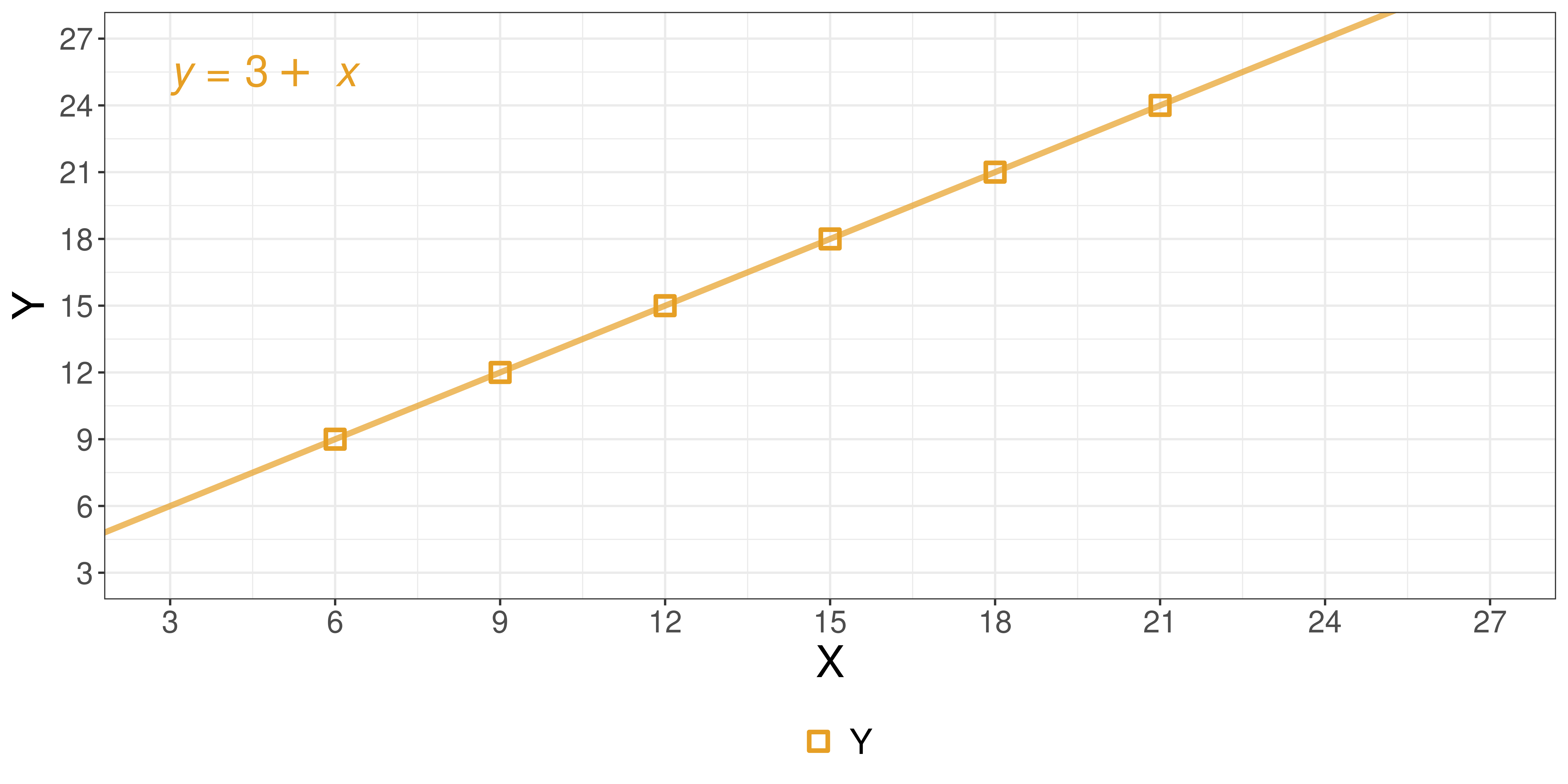
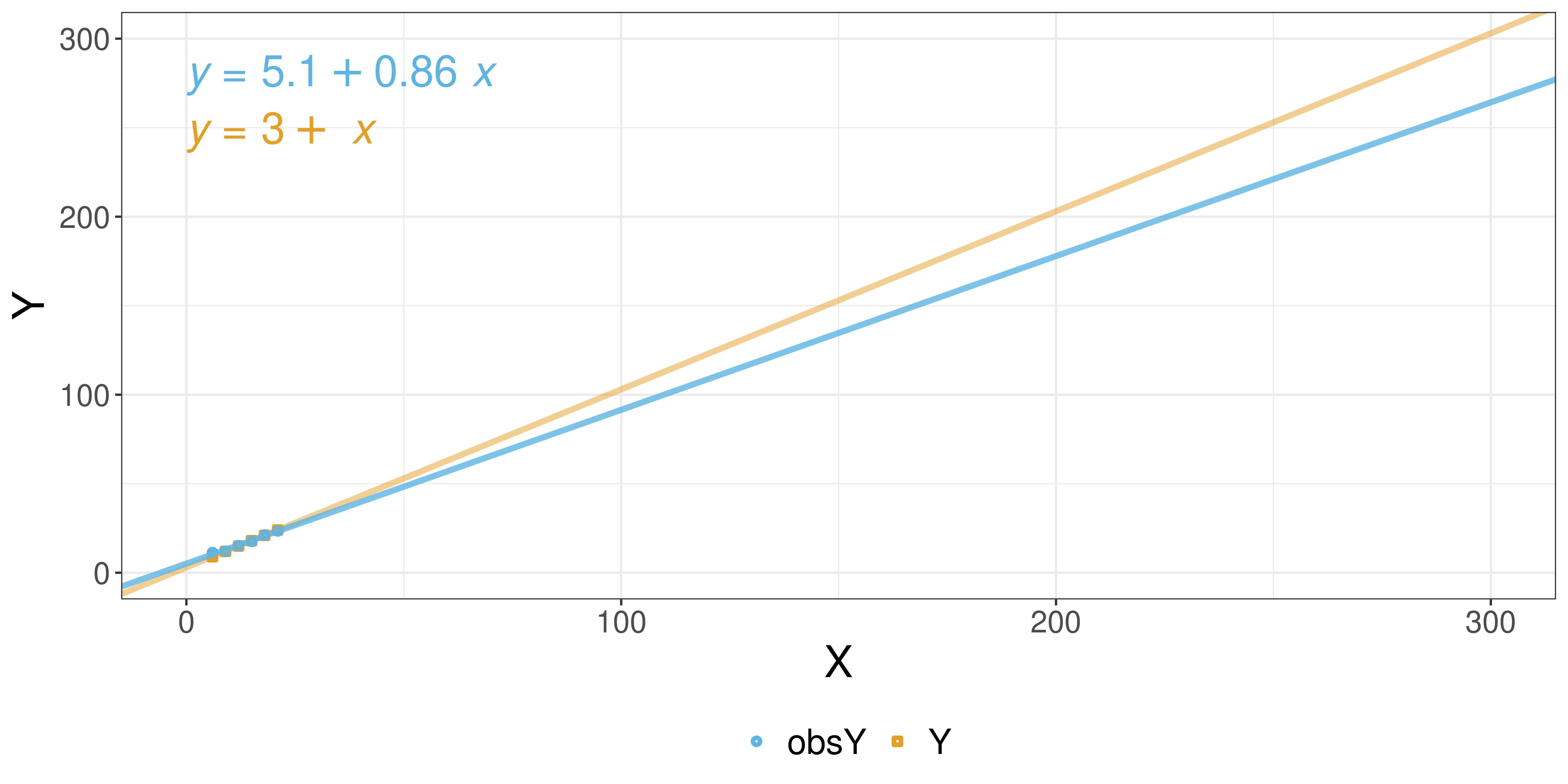
Visualizing the data

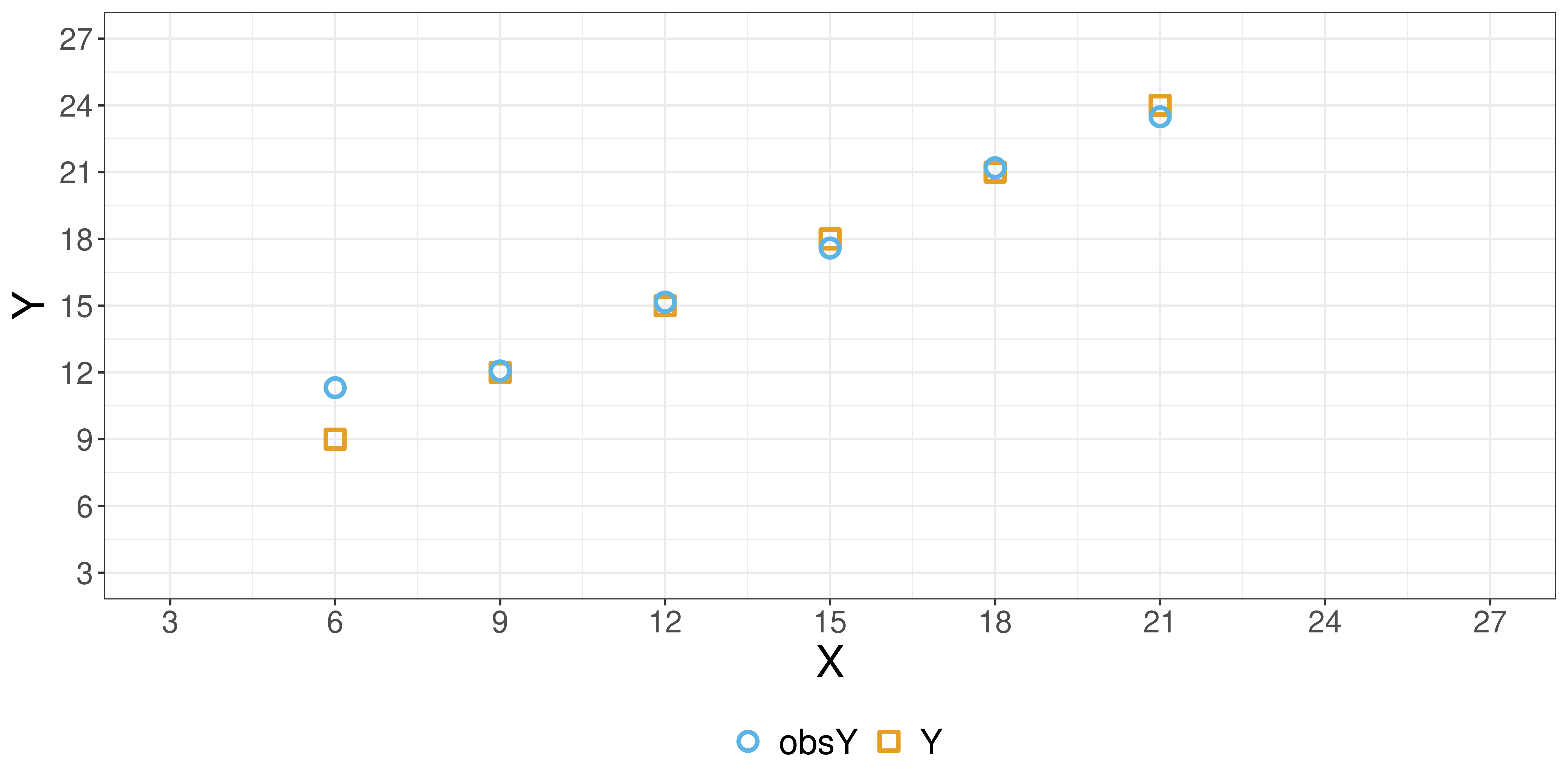
Visualizing the data (w/ noise)

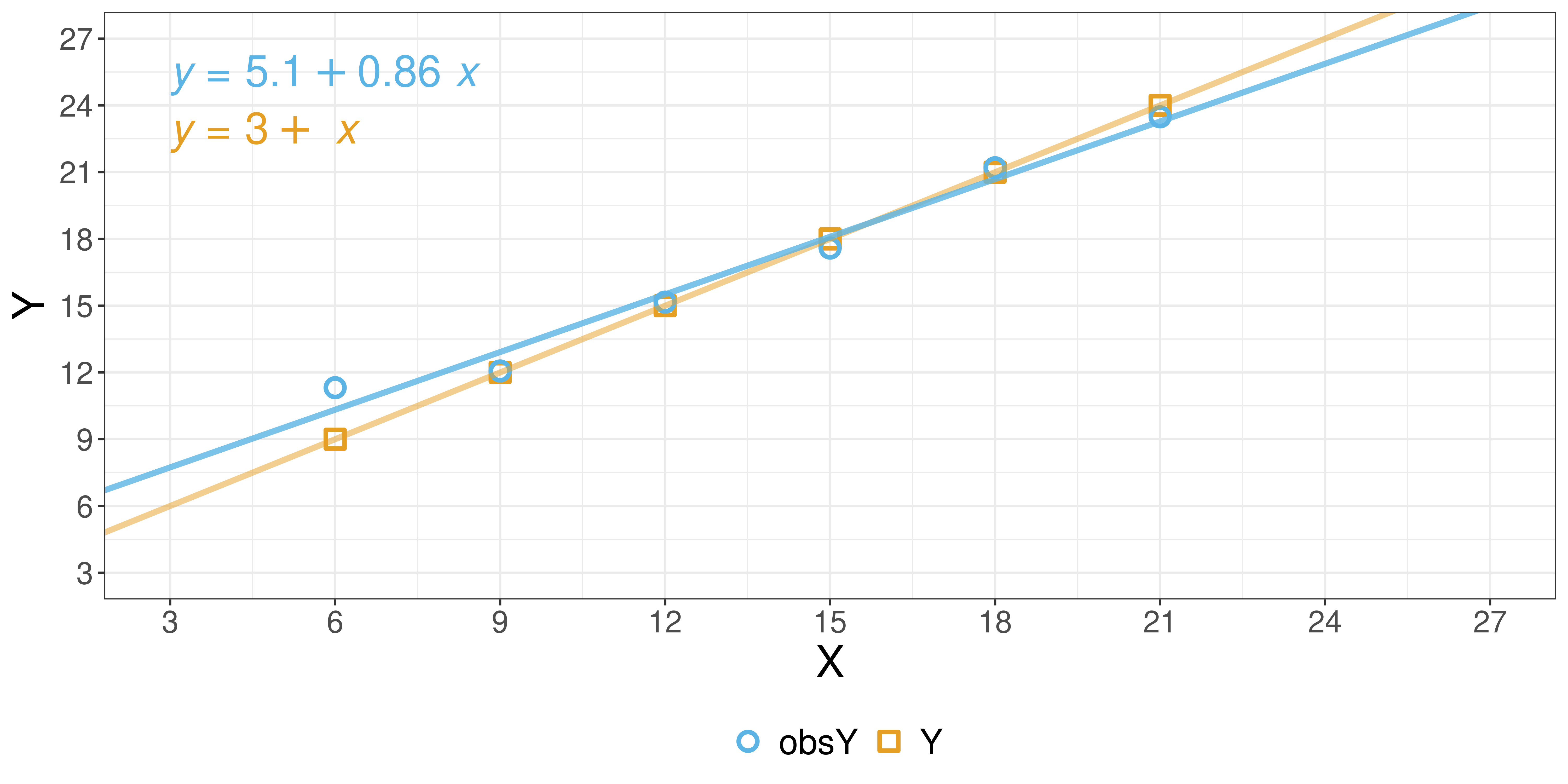
Visualizing the data (w/ noise)

Which line is closer to the “truth”?

Visualizing the data (w/ noise)

How much error can we accept?

Assessing error

How much error was introduced by \(\epsilon\) per sample?

df$error    <- df$Y - df$obsY  # Calculate the error
df$absError <- abs(df$error)   # Ignore the sign of error
df

# A tibble: 6 × 5
      X     Y  obsY   error absError
  <int> <int> <dbl>   <dbl>    <dbl>
1     6     9  11.3 -2.31     2.31  
2     9    12  12.1 -0.0662   0.0662
3    12    15  15.2 -0.162    0.162 
4    15    18  17.6  0.411    0.411 
5    18    21  21.2 -0.197    0.197 
6    21    24  23.5  0.513    0.513 

On average, what is the error?

mean(df$absError)

[1] 0.610755

This measure is called the Mean Absolute Error.

Measures of error

This is what we computed:

\[ \operatorname{MAE} = \frac{\sum_{i=1}^n{|(y_i + \epsilon) - y_i|}}{n} \]

• We were able to compute this error because we knew what the ground truth \(Y\), we knew what its real value was.
• It was only possible because it was a simulation, not real data.
• In practice, we will almost never be able to assess the impact of \(\epsilon\).
• We will use this same way of thinking to assess how good and accurate our models are. 🔜

What’s Next?

• We will introduce different measures of error and goodness-of-fit throughout this course.
• Next week we will cover Simple and Multiple Linear Regression
• Join our Slack group if you haven’t done so yet.
• Use the time before our first lab to revisit basic R programming skills.
• Head over to the 🔖 Week 01 - Appendix page for:
  • Indicative & recommended reading
  • Programming Resources

Thank you

References

Davenport, Thomas. 2020. “Beyond Unicorns: Educating, Classifying, and Certifying Business Data Scientists.” Harvard Data Science Review 2 (2). https://doi.org/10.1162/99608f92.55546b4a.

Schutt, Rachel, and Cathy O’Neil. 2013. Doing Data Science. First edition. Beijing ; Sebastopol: O’Reilly Media. https://ebookcentral.proquest.com/lib/londonschoolecons/detail.action?docID=1465965.

Shah, Chirag. 2020. A Hands-on Introduction to Data Science. Cambridge, United Kingdom ; New York, NY, USA: Cambridge University Press. https://librarysearch.lse.ac.uk/permalink/f/1n2k4al/TN_cdi_askewsholts_vlebooks_9781108673907.

Shmueli, Galit. 2010. “To Explain or to Predict?” Statistical Science 25 (3). https://doi.org/10.1214/10-STS330.