🗓️ Week 01 – Day 02
Data types and common file formats
09 Jul 2024
Datasets
📒 A dataset is simply a collection of data.
- But just having a bunch of data is not enough…
Important
Soon, you will start collecting data. If you’re not careful with how you organise it, you will end up with a mess that will be difficult to work with.
Garbage In -> Garbage Out
We need organised datasets
An example
Now we will start distinguishing:
- the types of data we can find in a dataset;
- the best practices to assemble a dataset.
Data Types
- Structured
- Unstructured
- Semi-structured
Structured Data
📒 Structured data is data that adheres to a pre-defined data model.
- As the name suggests, it has a structure.
- Tabular data is a common data structure ⏭️
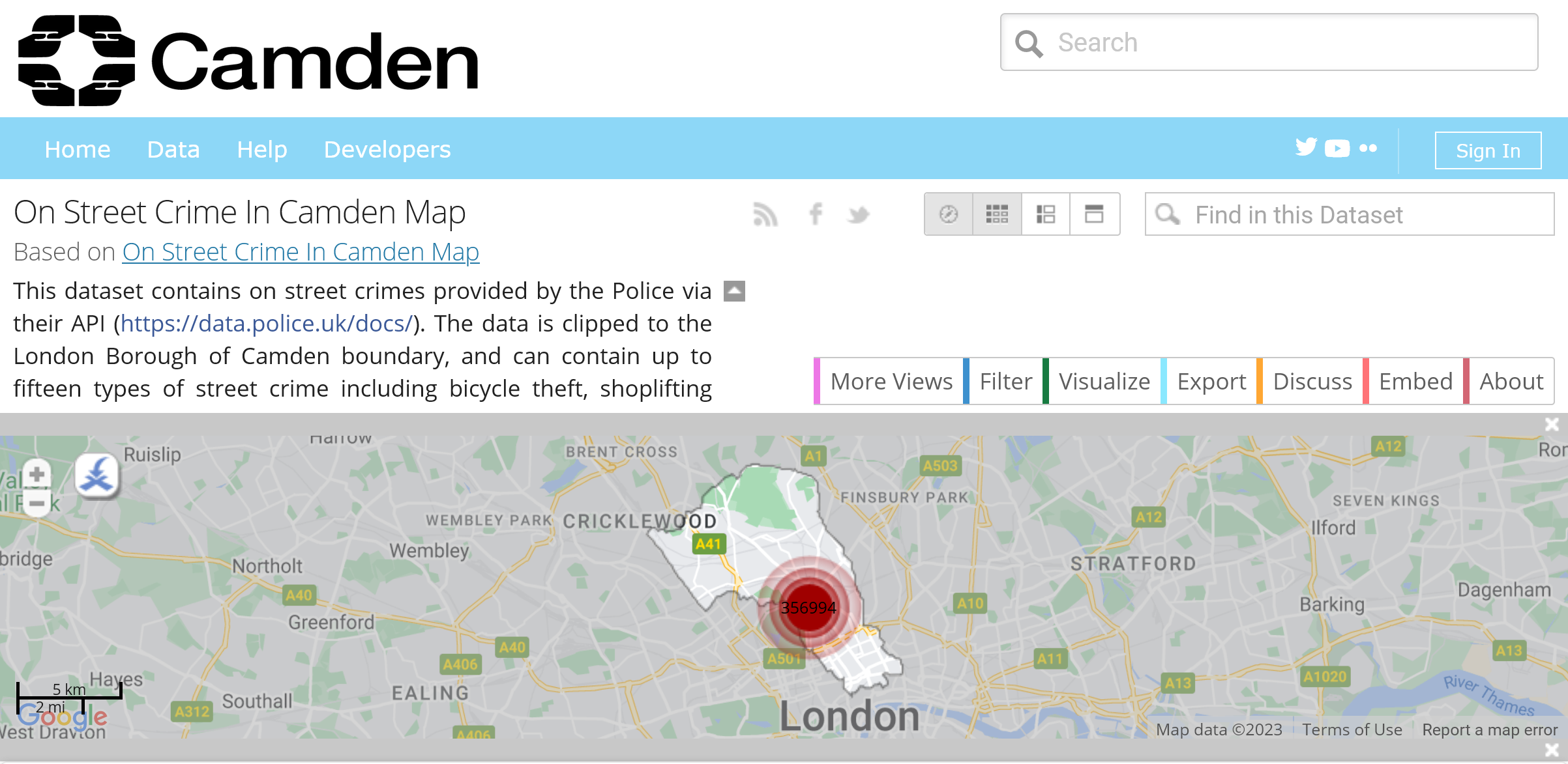
Example
Camden crime dataset
| Category | Street ID | Street Name | Outcome Category | Outcome Date |
|---|---|---|---|---|
| Other theft | 2344108 | Kings Cross (station) | Under investigation | 01/11/2022 |
| Other theft | 2343955 | Holborn (lu Station) | Under investigation | 01/11/2022 |
| Theft from the person | 2343569 | Euston (station) | Under investigation | 01/11/2022 |
| Shoplifting | 2344108 | Kings Cross (station) | Under investigation | 01/11/2022 |
| Public order | 2343101 | Camden Town (lu Station) | Under investigation | 01/11/2022 |
| Violence and sexual offences | 2343568 | Euston (lu Station) | Under investigation | 01/11/2022 |
| Other theft | 2344108 | Kings Cross (station) | Under investigation | 01/11/2022 |
| Public order | 2343164 | Chancery Lane (lu Station) | Under investigation | 01/11/2022 |
| Public order | 2343569 | Euston (station) | Under investigation | 01/11/2022 |
| Other theft | 2343569 | Euston (station) | Under investigation | 01/11/2022 |
| Theft from the person | 2343955 | Holborn (lu Station) | Under investigation | 01/11/2022 |
| Other theft | 2344108 | Kings Cross (station) | Under investigation | 01/11/2022 |
| Robbery | 2343623 | Finchley Road (lu Station) | Under investigation | 01/11/2022 |
| Theft from the person | 1678851 | On or near Shelton Street | Investigation complete; no suspect identified | 01/11/2022 |
Example (cont.)
Data type: numeric(*)
| Category | Street ID | Street Name | Outcome Category | Outcome Date |
|---|---|---|---|---|
| Other theft | 2344108 | Kings Cross (station) | Under investigation | 01/11/2022 |
| Other theft | 2343955 | Holborn (lu Station) | Under investigation | 01/11/2022 |
| Theft from the person | 2343569 | Euston (station) | Under investigation | 01/11/2022 |
| Shoplifting | 2344108 | Kings Cross (station) | Under investigation | 01/11/2022 |
| Public order | 2343101 | Camden Town (lu Station) | Under investigation | 01/11/2022 |
| Violence and sexual offences | 2343568 | Euston (lu Station) | Under investigation | 01/11/2022 |
| Other theft | 2344108 | Kings Cross (station) | Under investigation | 01/11/2022 |
| Public order | 2343164 | Chancery Lane (lu Station) | Under investigation | 01/11/2022 |
| Public order | 2343569 | Euston (station) | Under investigation | 01/11/2022 |
| Other theft | 2343569 | Euston (station) | Under investigation | 01/11/2022 |
| Theft from the person | 2343955 | Holborn (lu Station) | Under investigation | 01/11/2022 |
| Other theft | 2344108 | Kings Cross (station) | Under investigation | 01/11/2022 |
| Robbery | 2343623 | Finchley Road (lu Station) | Under investigation | 01/11/2022 |
| Theft from the person | 1678851 | On or near Shelton Street | Investigation complete; no suspect identified | 01/11/2022 |
* In R, use as.integer(df$column) or as.numeric(df$column) depending on the type of number you need.
* In Python, use df['column'].astype(int) or df['column'].astype(float).
Example (cont.)
Data type: string but could be treated as categorical(*)
| Category | Street ID | Street Name | Outcome Category | Outcome Date |
|---|---|---|---|---|
| Other theft | 2344108 | Kings Cross (station) | Under investigation | 01/11/2022 |
| Other theft | 2343955 | Holborn (lu Station) | Under investigation | 01/11/2022 |
| Theft from the person | 2343569 | Euston (station) | Under investigation | 01/11/2022 |
| Shoplifting | 2344108 | Kings Cross (station) | Under investigation | 01/11/2022 |
| Public order | 2343101 | Camden Town (lu Station) | Under investigation | 01/11/2022 |
| Violence and sexual offences | 2343568 | Euston (lu Station) | Under investigation | 01/11/2022 |
| Other theft | 2344108 | Kings Cross (station) | Under investigation | 01/11/2022 |
| Public order | 2343164 | Chancery Lane (lu Station) | Under investigation | 01/11/2022 |
| Public order | 2343569 | Euston (station) | Under investigation | 01/11/2022 |
| Other theft | 2343569 | Euston (station) | Under investigation | 01/11/2022 |
| Theft from the person | 2343955 | Holborn (lu Station) | Under investigation | 01/11/2022 |
| Other theft | 2344108 | Kings Cross (station) | Under investigation | 01/11/2022 |
| Robbery | 2343623 | Finchley Road (lu Station) | Under investigation | 01/11/2022 |
| Theft from the person | 1678851 | On or near Shelton Street | Investigation complete; no suspect identified | 01/11/2022 |
* In R, use as.factor(df$column) to convert a column to a categorical type.
* In Python, use df['column'].astype('category').
Example (cont.)
Data type: date(*)
| Category | Street ID | Street Name | Outcome Category | Outcome Date |
|---|---|---|---|---|
| Other theft | 2344108 | Kings Cross (station) | Under investigation | 01/11/2022 |
| Other theft | 2343955 | Holborn (lu Station) | Under investigation | 01/11/2022 |
| Theft from the person | 2343569 | Euston (station) | Under investigation | 01/11/2022 |
| Shoplifting | 2344108 | Kings Cross (station) | Under investigation | 01/11/2022 |
| Public order | 2343101 | Camden Town (lu Station) | Under investigation | 01/11/2022 |
| Violence and sexual offences | 2343568 | Euston (lu Station) | Under investigation | 01/11/2022 |
| Other theft | 2344108 | Kings Cross (station) | Under investigation | 01/11/2022 |
| Public order | 2343164 | Chancery Lane (lu Station) | Under investigation | 01/11/2022 |
| Public order | 2343569 | Euston (station) | Under investigation | 01/11/2022 |
| Other theft | 2343569 | Euston (station) | Under investigation | 01/11/2022 |
| Theft from the person | 2343955 | Holborn (lu Station) | Under investigation | 01/11/2022 |
| Other theft | 2344108 | Kings Cross (station) | Under investigation | 01/11/2022 |
| Robbery | 2343623 | Finchley Road (lu Station) | Under investigation | 01/11/2022 |
| Theft from the person | 1678851 | On or near Shelton Street | Investigation complete; no suspect identified | 01/11/2022 |
* The best way to deal with date-time data in R is to use the lubridate package. Base R date-time functions are NOT GREAT.
* In Python, use the pd.to_datetime(df['column']) function (but you might need to specify the format).
Text (data types)
- How is text represented in binary language?
- The ASCII table is one of early standards
- It encodes characters using 7-bits; therefore, it can represent a total of 128 unique characters
The ASCII table
| Dec | Binary | Char | Description |
|---|---|---|---|
| 0 | 0000000 | NUL | Null |
| 1 | 0000001 | SOH | Start of Header |
| 2 | 0000010 | STX | Start of Text |
| 3 | 0000011 | ETX | End of Text |
| 4 | 0000100 | EOT | End of Transmission |
| 5 | 0000101 | ENQ | Enquiry |
| 6 | 0000110 | ACK | Acknowledge |
| 7 | 0000111 | BEL | Bell |
| 8 | 0001000 | BS | Backspace |
| 9 | 0001001 | HT | Horizontal Tab |
| 10 | 0001010 | LF | Line Feed |
| 11 | 0001011 | VT | Vertical Tab |
| 12 | 0001100 | FF | Form Feed |
| 13 | 0001101 | CR | Carriage Return |
| 14 | 0001110 | SO | Shift Out |
| 15 | 0001111 | SI | Shift In |
| 16 | 0010000 | DLE | Data Link Escape |
| 17 | 0010001 | DC1 | Device Control 1 |
| 18 | 0010010 | DC2 | Device Control 2 |
| 19 | 0010011 | DC3 | Device Control 3 |
| 20 | 0010100 | DC4 | Device Control 4 |
| 21 | 0010101 | NAK | Negative Acknowledge |
| 22 | 0010110 | SYN | Synchronize |
| 23 | 0010111 | ETB | End of Transmission Block |
| 24 | 0011000 | CAN | Cancel |
| 25 | 0011001 | EM | End of Medium |
| 26 | 0011010 | SUB | Substitute |
| 27 | 0011011 | ESC | Escape |
| 28 | 0011100 | FS | File Separator |
| 29 | 0011101 | GS | Group Separator |
| 30 | 0011110 | RS | Record Separator |
| 31 | 0011111 | US | Unit Separator |
| Dec | Binary | Char | Description |
|---|---|---|---|
| 32 | 0100000 | space | Space |
| 33 | 0100001 | ! | exclamation mark |
| 34 | 0100010 | ” | double quote |
| 35 | 0100011 | # | number |
| 36 | 0100100 | $ | dollar |
| 37 | 0100101 | % | percent |
| 38 | 0100110 | & | ampersand |
| 39 | 0100111 | ’ | single quote |
| 40 | 0101000 | ( | left parenthesis |
| 41 | 0101001 | ) | right parenthesis |
| 42 | 0101010 | * | asterisk |
| 43 | 0101011 | + | plus |
| 44 | 0101100 | , | comma |
| 45 | 0101101 | - | minus |
| 46 | 0101110 | . | period |
| 47 | 0101111 | / | slash |
| 48 | 0110000 | 0 | zero |
| 49 | 0110001 | 1 | one |
| 50 | 0110010 | 2 | two |
| 51 | 0110011 | 3 | three |
| 52 | 0110100 | 4 | four |
| 53 | 0110101 | 5 | five |
| 54 | 0110110 | 6 | six |
| 55 | 0110111 | 7 | seven |
| 56 | 0111000 | 8 | eight |
| 57 | 0111001 | 9 | nine |
| 58 | 0111010 | : | colon |
| 59 | 0111011 | ; | semicolon |
| 60 | 0111100 | < | less than |
| 61 | 0111101 | = | equality sign |
| 62 | 0111110 | > | greater than |
| 63 | 0111111 | ? | question mark |
| Dec | Binary | Char | Description |
|---|---|---|---|
| 64 | 1000000 | @ | at sign |
| 65 | 1000001 | A | |
| 66 | 1000010 | B | |
| 67 | 1000011 | C | |
| 68 | 1000100 | D | |
| 69 | 1000101 | E | |
| 70 | 1000110 | F | |
| 71 | 1000111 | G | |
| 72 | 1001000 | H | |
| 73 | 1001001 | I | |
| 74 | 1001010 | J | |
| 75 | 1001011 | K | |
| 76 | 1001100 | L | |
| 77 | 1001101 | M | |
| 78 | 1001110 | N | |
| 79 | 1001111 | O | |
| 80 | 1010000 | P | |
| 81 | 1010001 | Q | |
| 82 | 1010010 | R | |
| 83 | 1010011 | S | |
| 84 | 1010100 | T | |
| 85 | 1010101 | U | |
| 86 | 1010110 | V | |
| 87 | 1010111 | W | |
| 88 | 1011000 | X | |
| 89 | 1011001 | Y | |
| 90 | 1011010 | Z | |
| 91 | 1011011 | [ | left square bracket |
| 92 | 1011100 | \ | backslash |
| 93 | 1011101 | ] | right square bracket |
| 94 | 1011110 | ^ | caret / circumflex |
| 95 | 1011111 | _ | underscore |
| Dec | Binary | Char | Description |
|---|---|---|---|
| 96 | 1100000 | ` | grave / accent |
| 97 | 1100001 | a | |
| 98 | 1100010 | b | |
| 99 | 1100011 | c | |
| 100 | 1100100 | d | |
| 101 | 1100101 | e | |
| 102 | 1100110 | f | |
| 103 | 1100111 | g | |
| 104 | 1101000 | h | |
| 105 | 1101001 | i | |
| 106 | 1101010 | j | |
| 107 | 1101011 | k | |
| 108 | 1101100 | l | |
| 109 | 1101101 | m | |
| 110 | 1101110 | n | |
| 111 | 1101111 | o | |
| 112 | 1110000 | p | |
| 113 | 1110001 | q | |
| 114 | 1110010 | r | |
| 115 | 1110011 | s | |
| 116 | 1110100 | t | |
| 117 | 1110101 | u | |
| 118 | 1110110 | v | |
| 119 | 1110111 | w | |
| 120 | 1111000 | x | |
| 121 | 1111001 | y | |
| 122 | 1111010 | z | |
| 123 | 1111011 | { | left curly bracket |
| 124 | 1111100 | ||
| 125 | 1111101 | } | right curly bracket |
| 126 | 1111110 | ~ | tilde |
| 127 | 1000001 | DEL | delete |
Other text formats
ASCII is not the only standard. There are other ways to encode text using binary.
Below is a non-comprehensive list of other text (encoding):
- Unicode
- UTF-8 (Most common of all)
- UTF-16
- UTF-32
- ISO-8859-1
- Latin-1
Note
💡 You might have come across encoding mismatches before if you ever opened a file and the text looked like this:
“Nestlé and Mötley Crüe”
Where it should have read
“Nestlé and Mötley Crüe”
Emojis 😀
Emojis are text! They are part of UTF-8
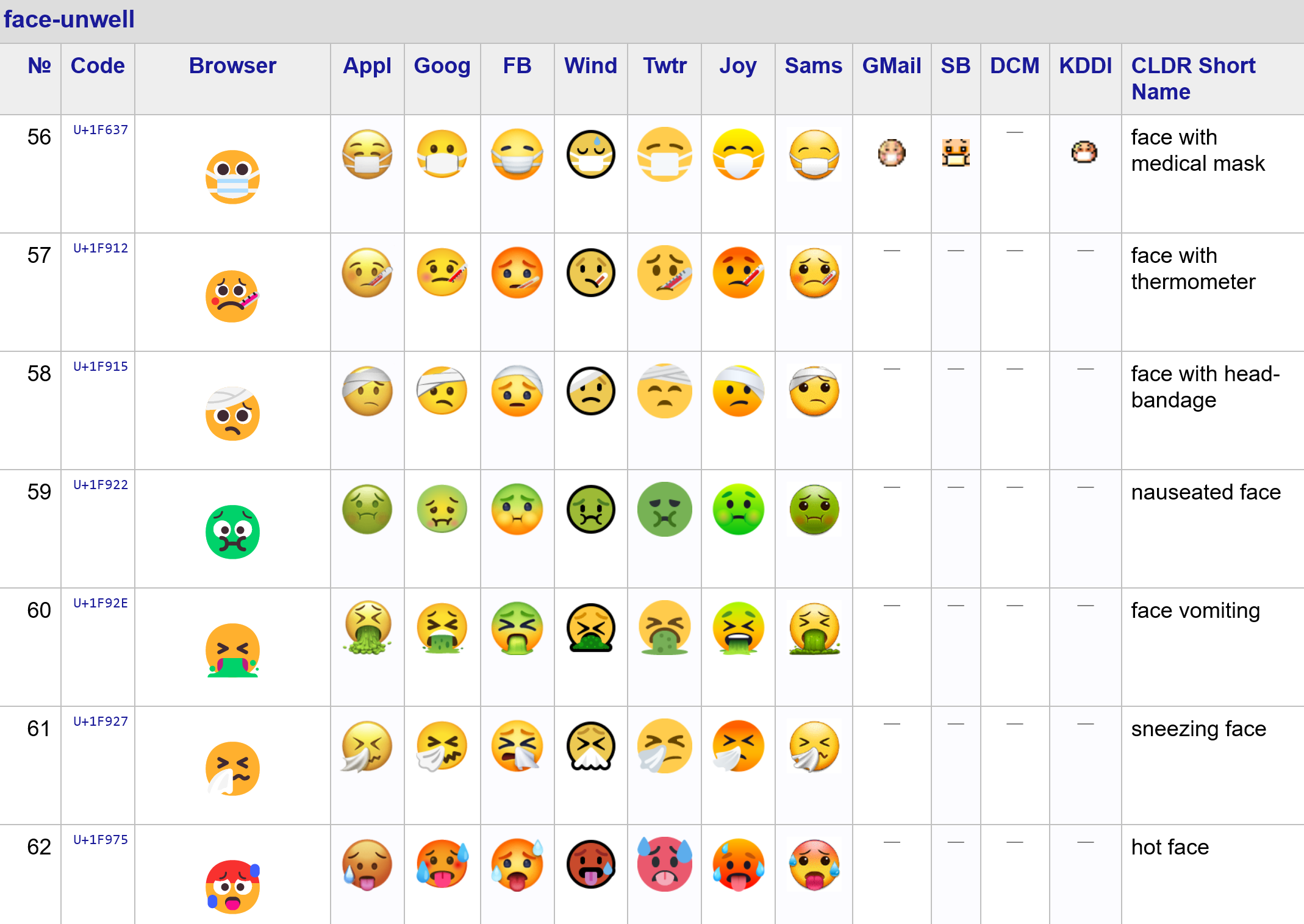
See the complete list on the Unicode website
Structured data can still be messy
- In this context, messy data refers to data that requires extensive preprocessing before it can be effectively used in:
- Exploratory data analysis,
- Statistical tools, or
- Training machine learning algorithms.
- It is important to establish standards to simplify our work.
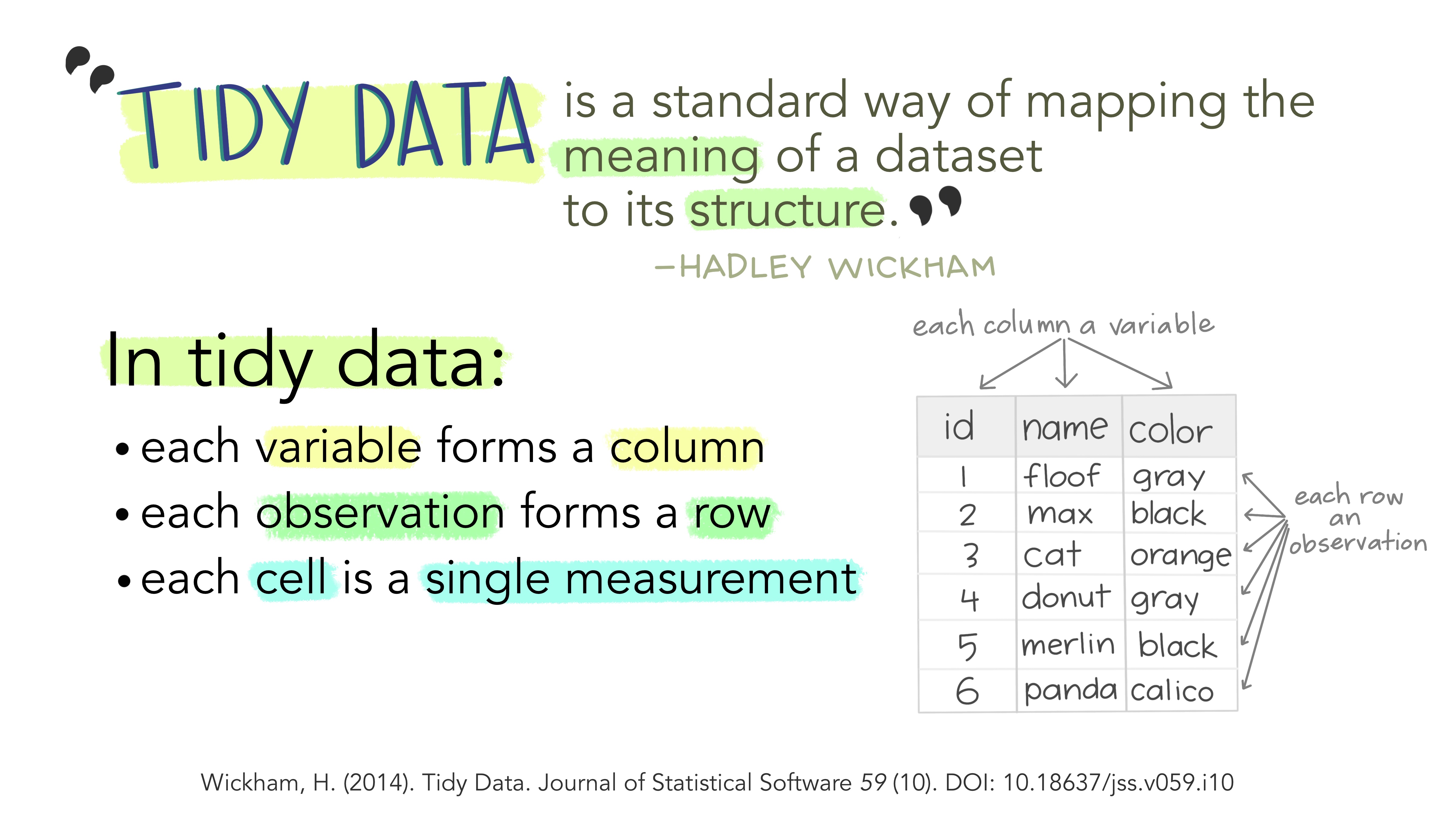
- One such standard for data handling is that of tidy data ➡️
What this means for you
- Most data you will collect will come “messy”
- but you can tidy it up using
tidyverse(R) orpandas(Python)
- but you can tidy it up using
- You will be asked over and over and over again to make your data tidy!
- tidy data will be a requirement for your coursework
Note
📘 Read more about tidy data
Wickham, H. . (2014). Tidy Data. Journal of Statistical Software, 59(10), 1–23. (Wickham 2014)
What about Unstructured Data?
📒 Unstructured data does NOT adhere to a pre-defined data model.
- Rule of thumb: it is not easy to think of this type of data as a table.
- Let’s see a few examples ➡️
Examples
Pure “raw” text

Photos

Videos

Text in scanned images
Semi-structured data
For example, e-mails:
- Parts of the data have a structure
- But the main content itself is usually just raw text
Note
Have you heard of the Enron e-mail scandal story before?

Common File Formats
I will show you how the following file formats are structured and how to read them in R:
- CSV
- XML
- JSON
CSV
- CSV stands for Comma Separated Values
CSV - Example
Which means a table like this:
| Category | Street ID | Street Name | Outcome Category | Outcome Date | Location |
|---|---|---|---|---|---|
| Other theft | 1489515 | Kings Cross (station) | Status update unavailable | 01/08/2017 | (51.5318, -0.123189) |
| Anti-social behaviour | 960522 | On or near Wellesley Place | (51.528169, -0.131558) | ||
| Theft from the person | 965233 | On or near Avenue Road | Investigation complete; no suspect identified | 01/08/2015 | (51.542741, -0.174124) |
| Anti-social behaviour | 960974 | On or near Birkenhead Street | (51.529611, -0.121652) | ||
| Drugs | 972275 | On or near Oakeshott Avenue | Offender given a drugs possession warning | 01/06/2015 | (51.565544, -0.149851) |
| Anti-social behaviour | 965090 | On or near Hawley Mews | (51.542507, -0.146589) | ||
| Violence and sexual offences | 967816 | On or near Maitland Park Villas | Under investigation | 01/06/2017 | (51.548264, -0.156365) |
| Vehicle crime | 967555 | On or near Ferncroft Avenue | Investigation complete; no suspect identified | 01/02/2016 | (51.558504, -0.191468) |
| Theft from the person | 965140 | On or near Nightclub | Under investigation | 01/04/2018 | (51.541352, -0.14629) |
| Other theft | 965052 | On or near Brocas Close | Investigation complete; no suspect identified | 01/05/2016 | (51.543954, -0.165408) |
CSV - Example
Becomes this:
Category,Street ID,Street Name,Outcome Category,Outcome Date,Location
Other theft,1489515,Kings Cross (station),Status update unavailable,01/08/2017,"(51.5318, -0.123189)"
Anti-social behaviour,960522,On or near Wellesley Place,,,"(51.528169, -0.131558)"
Theft from the person,965233,On or near Avenue Road,Investigation complete; no suspect identified,01/08/2015,"(51.542741, -0.174124)"
Anti-social behaviour,960974,On or near Birkenhead Street,,,"(51.529611, -0.121652)"
Drugs,972275,On or near Oakeshott Avenue,Offender given a drugs possession warning,01/06/2015,"(51.565544, -0.149851)"
Anti-social behaviour,965090,On or near Hawley Mews,,,"(51.542507, -0.146589)"
Violence and sexual offences,967816,On or near Maitland Park Villas,Under investigation,01/06/2017,"(51.548264, -0.156365)"
Vehicle crime,967555,On or near Ferncroft Avenue,Investigation complete; no suspect identified,01/02/2016,"(51.558504, -0.191468)"
Theft from the person,965140,On or near Nightclub,Under investigation,01/04/2018,"(51.541352, -0.14629)"
Other theft,965052,On or near Brocas Close,Investigation complete; no suspect identified,01/05/2016,"(51.543954, -0.165408)"
CSV - Example
- CSV files encode tabular data, so it is easy to read them into a data frame.
R
Tip
Read more about Common CSV Problems.
CSV - Inspecting data types (R)
You can use
str(csv_data)to inspect data types.On base R, you will get something like this:
'data.frame':   376132 obs. of  20 variables:
 $ Category        : chr  "Other theft" "Anti-social behaviour" "Theft from the person" "Anti-social behaviour" ...
 $ Street.ID       : int  1489515 960522 965233 960974 972275 965090 967816 967555 965140 965052 ...
 $ Street.Name     : chr  "Kings Cross (station)" "On or near Wellesley Place" "On or near Avenue Road" "On or nea.
 $ Context         : logi  NA NA NA NA NA NA ...
 $ Outcome.Category: chr  "Status update unavailable" "" "Investigation complete; no suspect identified" "" ...
 $ Outcome.Date    : chr  "01/08/2017" "" "01/08/2015" "" ...
 $ Service         : chr  "British Transport Police" "Police Force" "Police Force" "Police Force" ...
 $ Location.Subtype: chr  "Station" "" "" "" ...
 $ ID              : int  64777250 51520755 42356413 59431385 41931981 51522064 58014826 46231592 64334450 4850859.
 $ Persistent.ID   : chr  "" "" "915131bf174019fd2fcf5aa4af305f7b2b34a763d8fcb0ccc4050503b82fa0fb" "" ...
 $ Epoch           : chr  "01/04/2017" "01/09/2016" "01/07/2015" "01/08/2017" ...
 $ Ward.Code       : chr  "E05000143" "E05000143" "E05000144" "E05000141" ...
 $ Ward.Name       : chr  "St Pancras and Somers Town" "St Pancras and Somers Town" "Swiss Cottage" "King's Cross".
 $ Easting         : num  530277 529707 526717 530390 528336 ...
 $ Northing        : num  183101 182683 184228 182861 186806 ...
 $ Longitude       : num  -0.123 -0.132 -0.174 -0.122 -0.15 ...
 $ Latitude        : num  51.5 51.5 51.5 51.5 51.6 ...
 $ Spatial.Accuracy: chr  "This is only an approximation of where the crime happened" "This is only an approximati.
 $ Last.Uploaded   : chr  "11/07/2018" "11/07/2018" "05/05/2016" "03/11/2017" ...
 $ Location        : chr  "(51.5318, -0.123189)" "(51.528169, -0.131558)" "(51.542741, -0.174124)" "(51.529611, -0.
R is pretty good at guessing data types, but it won’t get things like dates right and it won’t always use the most efficient data type (e.g. int vs num).
CSV - Inspecting data types (tidyverse)
- If you read the data frame with tidyverse,
str(csv_data)will look differently:
spc_tbl_ [376,132 x 20] (S3: spec_tbl_df/tbl_df/tbl/data.frame)
 $ Category        : chr [1:376132] "Other theft" "Anti-social behaviour" "Theft from the person" "Anti-social beh.
 $ Street ID       : num [1:376132] 1489515 960522 965233 960974 972275 ...
 $ Street Name     : chr [1:376132] "Kings Cross (station)" "On or near Wellesley Place" "On or near Avenue Road" .
 $ Context         : logi [1:376132] NA NA NA NA NA NA ...
 $ Outcome Category: chr [1:376132] "Status update unavailable" NA "Investigation complete; no suspect identified".
 $ Outcome Date    : chr [1:376132] "01/08/2017" NA "01/08/2015" NA ...
 $ Service         : chr [1:376132] "British Transport Police" "Police Force" "Police Force" "Police Force" ...
 $ Location Subtype: chr [1:376132] "Station" NA NA NA ...
 $ ID              : num [1:376132] 64777250 51520755 42356413 59431385 41931981 ...
 $ Persistent ID   : chr [1:376132] NA NA "915131bf174019fd2fcf5aa4af305f7b2b34a763d8fcb0ccc4050503b82fa0fb" NA ...
 $ Epoch           : chr [1:376132] "01/04/2017" "01/09/2016" "01/07/2015" "01/08/2017" ...
 $ Ward Code       : chr [1:376132] "E05000143" "E05000143" "E05000144" "E05000141" ...
 $ Ward Name       : chr [1:376132] "St Pancras and Somers Town" "St Pancras and Somers Town" "Swiss Cottage" "Kin.
 $ Easting         : num [1:376132] 530277 529707 526717 530390 528336 ...
 $ Northing        : num [1:376132] 183101 182683 184228 182861 186806 ...
 $ Longitude       : num [1:376132] -0.123 -0.132 -0.174 -0.122 -0.15 ...
 $ Latitude        : num [1:376132] 51.5 51.5 51.5 51.5 51.6 ...
 $ Spatial Accuracy: chr [1:376132] "This is only an approximation of where the crime happened" "This is only an a.
 $ Last Uploaded   : chr [1:376132] "11/07/2018" "11/07/2018" "05/05/2016" "03/11/2017" ...
 $ Location        : chr [1:376132] "(51.5318, -0.123189)" "(51.528169, -0.131558)" "(51.542741, -0.174124)" "(51..
 - attr(*, "spec")=
  .. cols(
  ..   Category = col_character(),
  ..   `Street ID` = col_double(),
  ..   `Street Name` = col_character(),
  ..   Context = col_logical(),
  ..   `Outcome Category` = col_character(),
  ..   `Outcome Date` = col_character(),
  ..   Service = col_character(),
  ..   `Location Subtype` = col_character(),
  ..   ID = col_double(),
  ..   `Persistent ID` = col_character(),
  ..   Epoch = col_character(),
  ..   `Ward Code` = col_character(),
  ..   `Ward Name` = col_character(),
  ..   Easting = col_double(),
  ..   Northing = col_double(),
  ..   Longitude = col_double(),
  ..   Latitude = col_double(),
  ..   `Spatial Accuracy` = col_character(),
  ..   `Last Uploaded` = col_character(),
  ..   Location = col_character()
  .. )
 - attr(*, "problems")=<externalptr>
CSV - Inspecting data types (tidyverse)
In sum:
- the output is more verbose
tidyversedidn’t useinteven in the most explicit cases (e.g.Street ID)- it used
numinstead
- it used
- similarly, it didn’t use
factorsfor obviously categorical variables
(e.g.Outcome Category) - it didn’t decode the dates (e.g.
Outcome Date)
But I really want to draw your attention to the following line:
which indicates that this is a ![]() tibble object.
tibble object.
From the tibble documentation:
A tibble, or
tbl_df, is a modern reimagining of the data.frame, keeping what time has proven to be effective, and throwing out what is not.Tibbles are data.frames that are lazy and surly:
- they do less (i.e. they don’t change variable names or types, and don’t do partial matching)
- and complain more (e.g. when a variable does not exist).
This forces you to confront problems earlier, typically leading to cleaner, more expressive code. Tibbles also have an enhanced print() method which makes them easier to use with large datasets containing complex objects.
If you are new to tibbles, the best place to start is the tibbles chapter in R for data science (Wickham and Grolemund 2016, chap. 10).
Source: the documentation page of tibble, accessed on 08 July 2023.. I have split the paragraphs and highlighted certain words for better communication.
CSV - Inspecting data types (Python)
You can use
csv_data.dtypesto inspect data types.In
pandas, you will get something like this:
Category             object
Street ID             int64
Street Name          object
Context             float64
Outcome Category     object
Outcome Date         object
Service              object
Location Subtype     object
ID                    int64
Persistent ID        object
Epoch                object
Ward Code            object
Ward Name            object
Easting             float64
Northing            float64
Longitude           float64
Latitude            float64
Spatial Accuracy     object
Last Uploaded        object
Location             object
dtype: object
CSV - Inspecting data types (df.info())
In sum:
- the output is more verbose
pandasdidn’t use the most memory-efficientint- it used
int64even for small ranges
- it used
- similarly, it didn’t use
categoryfor obviously categorical variables
(e.g.Outcome Category) - it didn’t decode the dates (e.g.
Outcome Date)
Category             object
<class 'pandas.core.frame.DataFrame'>
RangeIndex: 419273 entries, 0 to 419272
Data columns (total 20 columns):
 #   Column            Non-Null Count   Dtype
---  ------            --------------   -----
 0   Category          419273 non-null  object
 1   Street ID         419273 non-null  int64
 2   Street Name       419273 non-null  object
 3   Context           0 non-null       float64
 4   Outcome Category  324353 non-null  object
 5   Outcome Date      324353 non-null  object
 6   Service           419273 non-null  object
 7   Location Subtype  15697 non-null   object
 8   ID                419273 non-null  int64
 9   Persistent ID     298195 non-null  object
 10  Epoch             419273 non-null  object
 11  Ward Code         419273 non-null  object
 12  Ward Name         419273 non-null  object
 13  Easting           419273 non-null  float64
 14  Northing          419273 non-null  float64
 15  Longitude         419273 non-null  float64
 16  Latitude          419273 non-null  float64
 17  Spatial Accuracy  419273 non-null  object
 18  Last Uploaded     419273 non-null  object
 19  Location          419273 non-null  object
dtypes: float64(5), int64(2), object(13)
memory usage: 64.0+ MB
Our approach to data processing
- This philosophy aligns with the principles of this course.
- We want you using the most appropriate data types and addressing issues proactively early on.
- Even if they are not super necessary (i.e. you don’t have Big Data)
- From a pedagogical standpoint, it is crucial for us to teach you the best practices.
- Let me be more specific ➡️
Principle 1: Ensure data types make sense (R)
Reflect on the character variables (R)
- How many unique values each of them have?
csv_data %>%
  select(where(is.character)) %>%
  summarise(across(everything(), n_distinct)) %>%
  pivot_longer(everything(),
               names_to = "Column",
               values_to = "# Distinct") %>%
  mutate(Percentage=sprintf("%.2f%%",(`# Distinct`/dim(csv_data)[1])*100)) %>%
  arrange(desc(`# Distinct`))
🗣️ CLASS DISCUSSION
What does this summary tell us?
| Column | # Distinct | Percentage |
|---|---|---|
| Persistent ID | 257160 | 68.37% |
| Location | 2917 | 0.78% |
| Street Name | 1311 | 0.35% |
| Outcome Date | 101 | 0.03% |
| Epoch | 100 | 0.03% |
| Ward Code | 38 | 0.01% |
| Outcome Category | 27 | 0.01% |
| Ward Name | 27 | 0.01% |
| Last Uploaded | 27 | 0.01% |
| Category | 14 | 0.00% |
| Location Subtype | 3 | 0.00% |
| Service | 2 | 0.00% |
| Spatial Accuracy | 1 | 0.00% |
🛣️ First, let’s take a little detour to understand the code above.
🛣️ Detour: Code explainer
First, we select only the character variables.
🛣️ Detour: Code explainer (R)
Then we summarise each selected column using the across() function.
This returns the following tibble:
# A tibble: 1 x 13
  Category `Street Name` `Outcome Category` `Outcome Date` Service `Location Subtype` `Persistent ID` Epoch `Ward Code` `Ward Name`
     <int>         <int>              <int>          <int>   <int>              <int>           <int> <int>       <int>       <int>
1       14          1311                 27            101       2                  3          257160   100          38          27
# i 3 more variables: `Spatial Accuracy` <int>, `Last Uploaded` <int>, Location <int>
🛣️ Detour: Code explainer (R)
We use the pivot_longer() function from the tidyr package to ‘rotate’ the data:
Columns becomes rows:
🛣️ Detour: Code explainer (R)
Now it’s easy to add a new column with the percentages using mutate:
This produces:
# A tibble: 13 x 3
   Column           `# Distinct` Percentage
   <chr>                   <int> <chr>
 1 Category                   14 0.00%
 2 Street Name              1311 0.35%
 3 Outcome Category           27 0.01%
 4 Outcome Date              101 0.03%
 5 Service                     2 0.00%
 6 Location Subtype            3 0.00%
 7 Persistent ID          257160 68.37%
 8 Epoch                     100 0.03%
 9 Ward Code                  38 0.01%
10 Ward Name                  27 0.01%
11 Spatial Accuracy            1 0.00%
12 Last Uploaded              27 0.01%
13 Location                 2917 0.78%
🛣️ Detour: Code explainer (R)
To communicate the results better, we sort the rows by # Distinct:
which leads us to our desired output:
# A tibble: 13 x 3
   Column           `# Distinct` Percentage
   <chr>                   <int> <chr>
 1 Persistent ID          257160 68.37%
 2 Location                 2917 0.78%
 3 Street Name              1311 0.35%
 4 Outcome Date              101 0.03%
 5 Epoch                     100 0.03%
 6 Ward Code                  38 0.01%
 7 Outcome Category           27 0.01%
 8 Ward Name                  27 0.01%
 9 Last Uploaded              27 0.01%
10 Category                   14 0.00%
11 Location Subtype            3 0.00%
12 Service                     2 0.00%
13 Spatial Accuracy            1 0.00%
Peek at the data
🗣️ How would you change the type of these columns?
| Persistent ID | Location | Street Name | Service | Spatial Accuracy |
|---|---|---|---|---|
| NA | (51.5318, -0.123189) | Kings Cross (station) | British Transport Police | This is only an approx |
| NA | (51.528169, -0.131558) | On or near Wellesley Place | Police Force | This is only an approx |
| 915131bf174019fd2fcf5aa4af305f7b2b34a763d8fcb0ccc4050503b82fa0fb | (51.542741, -0.174124) | On or near Avenue Road | Police Force | This is only an approx |
| NA | (51.529611, -0.121652) | On or near Birkenhead Street | Police Force | This is only an approx |
| bd5bef6ee7b3711e69ecfc40c1c256d45336f23aeda337b24616efed2eafddf1 | (51.565544, -0.149851) | On or near Oakeshott Avenue | Police Force | This is only an approx |
| NA | (51.542507, -0.146589) | On or near Hawley Mews | Police Force | This is only an approx |
| 32d289676240e51a8f0adcb1fd796547820cd59d5dcdeb6e1f6678d21dce9865 | (51.548264, -0.156365) | On or near Maitland Park Villas | Police Force | This is only an approx |
| 6149304809fb465afd840bd6a35bdfac1a06915d2bcb2baa7361719e5467d8bd | (51.558504, -0.191468) | On or near Ferncroft Avenue | Police Force | This is only an approx |
| 34795948a0731cd1f445b59eb237e93146a784f108a81bceccfea8e2ffcd91d5 | (51.541352, -0.14629) | On or near Nightclub | Police Force | This is only an approx |
| 05d796c77702b5cd2f5c03c32ff51c49c95a7ecc0f4f404a701e141ece858160 | (51.543954, -0.165408) | On or near Brocas Close | Police Force | This is only an approx |
| NA | (51.5325, -0.12601) | St Pancras International (station) | British Transport Police | This is only an approx |
| da582a168109e9c5e41f06add7c629083f0d5cd9ed0da5679732cce1fab9f6fe | (51.524465, -0.124891) | On or near Marchmont Street | Police Force | This is only an approx |
| 8c71420dfdcee3dc390e78791189d931f72ed677a510f377e274dfd0cf205c29 | (51.545363, -0.133277) | On or near Petrol Station | Police Force | This is only an approx |
| 8421b68d78559638e4bb243feb673a076b145a44e9da98cd91f289560509b109 | (51.541133, -0.192229) | On or near Quex Road | Police Force | This is only an approx |
| adef0ec085796c97a9dbca411af4b41adc33838025e704862cbb56580558827a | (51.545807, -0.162579) | On or near Supermarket | Police Force | This is only an approx |
| f374661faf45420007111e26473b5812c0ad22326e1e13aeece0c862467d3dda | (51.54288, -0.147425) | On or near Petrol Station | Police Force | This is only an approx |
| 29b4b7f0a8e2a31a5be0dafe0003b25d57ab0b41695f92064f6d185e9d78919a | (51.523469, -0.126114) | On or near Parking Area | Police Force | This is only an approx |
| 5416cc3cb894805a81221f43a42a47042a7c5baadf0871a43d04d8023e337718 | (51.552811, -0.135698) | On or near Montpelier Grove | Police Force | This is only an approx |
| 4e70cb3468ee72ab29bbadfb8141a6ea2ed04f1c2470d0890d1df6c4eeaaa500 | (51.540012, -0.151997) | On or near Edis Street | Police Force | This is only an approx |
| 3dc9881558b7c0d56141a49baf1afd1ce06abe0b6a78d393c972df50e240b714 | (51.545174, -0.194145) | On or near Gladys Road | Police Force | This is only an approx |
| e7f17dc1694fd5e79b0845f155bcf8d1f06cf849e182dc4c263982b57e0f12d9 | (51.548622, -0.20086) | On or near Barlow Road | Police Force | This is only an approx |
| ecc285067c5653ee74b31b52d94b5ff25b7086773bf9f8f4d427685259462888 | (51.544104, -0.149754) | On or near Mead Close | Police Force | This is only an approx |
| f22771d69e7ab3c163b1e095d6af93af2ec93d4979262f591f0116e3951bfeb3 | (51.538704, -0.141509) | On or near Greenland Place | Police Force | This is only an approx |
| 152d6dc7d7830074f58a93b37547e514b52f56bc032a03f72a01e99cf9739b93 | (51.539681, -0.142998) | On or near Nightclub | Police Force | This is only an approx |
| 042b4e6d44c1dc6b57b7fbdb992ec7bc36ee9640084ad44221e486c7e18e329d | (51.518544, -0.119008) | On or near Yorkshire Grey Yard | Police Force | This is only an approx |
Convert to categorical (factor) (R)
- Normally, whenever the number of unique values is small, consider converting the variable to a
factor. - But pay attention to the context.
- Never convert dates to
factor! - Also probably not a good idea to convert
IDvariables tofactor!
- Never convert dates to
Object sizes after conversion (R)
How many bytes does the csv_data object occupy in memory?
returns:
"99.5 Mb"And after converting selected columns to categorical?
selected_columns <- c("Spatial Accuracy", "Service", "Location Subtype",
                      "Category", "Ward Name", "Outcome Category", "Ward Code")

csv_data <- csv_data %>%
  mutate(across(all_of(selected_columns), factor))

format(object.size(csv_data), units = "auto")
returns:
"89.4 Mb"Tip
A reduction of \(10.1\%\) might not seem significant for a ‘small’ dataset, but remember: we’re building the habit of using the most efficient and most appropriate data types.
Use the forcats package (R)
- The
![]() forcats package has useful functions for working with factors.
forcats package has useful functions for working with factors.
Example: Counting the number of occurrences of each level with fct_count()
yields:
Convert to Date objects (R)
Welcome to yet another tidyverse package: ![]() lubridate.
lubridate.
What can you do with lubridate? (R)
This time we didn’t save much on memory, but we gained a lot in terms of flexibility.
selected_columns <- c("Last Uploaded", "Epoch", "Outcome Date")

csv_data <-
  csv_data %>%
  mutate(across(all_of(selected_columns), lubridate::dmy))

format(object.size(csv_data), units = "auto")
returns the same as before
"89.4 Mb"➡️ Let’s check out lubridate’s cheat sheet to see what we can do with dates: lubridate
Finally, let’s spot truly int variables (R)
Important
is.integer() DOES NOT test if the number can be safely converted to an integer.
- We can read about it in the relevant R documentation:
Finally, let’s spot truly int variables
- Let’s then convert the necessary columns to
integer:
Our current data frame
returns:
tibble [376,132 x 20] (S3: tbl_df/tbl/data.frame)
 $ Category        : Factor w/ 14 levels "Anti-social behaviour",..: 7 1 12 1 5 1 14 13 12 7 ...
 $ Street ID       : int [1:376132] 1489515 960522 965233 960974 972275 965090 967816 967555 965140 965052 ...
 $ Street Name     : chr [1:376132] "Kings Cross (station)" "On or near Wellesley Place" "On or near Avenue Road" "On or near Birkenhead Street" ...
 $ Context         : logi [1:376132] NA NA NA NA NA NA ...
 $ Outcome Category: Factor w/ 26 levels "Action to be taken by another organisation",..: 23 NA 9 NA 14 NA 26 9 26 9 ...
 $ Outcome Date    : Date[1:376132], format: "2017-08-01" NA "2015-08-01" NA ...
 $ Service         : Factor w/ 2 levels "British Transport Police",..: 1 2 2 2 2 2 2 2 2 2 ...
 $ Location Subtype: Factor w/ 2 levels "London Underground Station",..: 2 NA NA NA NA NA NA NA NA NA ...
 $ ID              : int [1:376132] 64777250 51520755 42356413 59431385 41931981 51522064 58014826 46231592 64334450 48508596 ...
 $ Persistent ID   : chr [1:376132] NA NA "915131bf174019fd2fcf5aa4af305f7b2b34a763d8fcb0ccc4050503b82fa0fb" NA ...
 $ Epoch           : Date[1:376132], format: "2017-04-01" "2016-09-01" "2015-07-01" "2017-08-01" ...
 $ Ward Code       : Factor w/ 38 levels "E05000128","E05000129",..: 16 16 17 14 10 3 9 6 3 1 ...
 $ Ward Name       : Factor w/ 27 levels "Belsize","Bloomsbury",..: 25 25 26 19 13 5 12 9 5 1 ...
 $ Easting         : num [1:376132] 530277 529707 526717 530390 528336 ...
 $ Northing        : num [1:376132] 183101 182683 184228 182861 186806 ...
 $ Longitude       : num [1:376132] -0.123 -0.132 -0.174 -0.122 -0.15 ...
 $ Latitude        : num [1:376132] 51.5 51.5 51.5 51.5 51.6 ...
 $ Spatial Accuracy: Factor w/ 1 level "This is only an approximation of where the crime happened": 1 1 1 1 1 1 1 1 1 1 ...
 $ Last Uploaded   : Date[1:376132], format: "2018-07-11" "2018-07-11" "2016-05-05" "2017-11-03" ...
 $ Location        : chr [1:376132] "(51.5318, -0.123189)" "(51.528169, -0.131558)" "(51.542741, -0.174124)" "(51.529611, -0.121652)" ...
Principle 1: Ensure data types make sense (Python)
Reflect on the object variables (Python)
- How many unique values each of them have?
(
  df_street_crime
    .select_dtypes(include=['object'])
    .nunique()
    .sort_values(ascending=False)
    .assign(Percentage=lambda x: x/x.sum())
    .to_frame(name='# Distinct')
    .style.format({'Percentage': '{:.2%}'})
)
🗣️ CLASS DISCUSSION
What does this summary tell us?
| Column | # Distinct | Percentage |
|---|---|---|
| Persistent ID | 257160 | 68.37% |
| Location | 2917 | 0.78% |
| Street Name | 1311 | 0.35% |
| Outcome Date | 101 | 0.03% |
| Epoch | 100 | 0.03% |
| Ward Code | 38 | 0.01% |
| Outcome Category | 27 | 0.01% |
| Ward Name | 27 | 0.01% |
| Last Uploaded | 27 | 0.01% |
| Category | 14 | 0.00% |
| Location Subtype | 3 | 0.00% |
| Service | 2 | 0.00% |
| Spatial Accuracy | 1 | 0.00% |
🛣️ First, let’s take a little detour to understand the code above.
🛣️ Detour: Code explainer (Python)
First, we select only the object variables.
🛣️ Detour: Code explainer (Python)
Then we count the number of unique values each selected column using the .nunique() method and sort them in descending order:
🛣️ Detour: Code explainer (Python)
We use the .assign() method to calculate the percentage of each column using an anonymous lambda function:
🛣️ Detour: Code explainer (Python)
We then convert the result to an html-formatted data frame using the .to_frame() method and format the Percentage column to shorten the decimal places:
This returns the following table:
| # Distinct | Percentage | |
|---|---|---|
| Persistent ID | 286221 | 98.41% |
| Location | 2936 | 1.01% |
| Street Name | 1317 | 0.45% |
| Outcome Date | 111 | 0.04% |
| Epoch | 111 | 0.04% |
| Ward Code | 38 | 0.01% |
| Last Uploaded | 36 | 0.01% |
| Ward Name | 27 | 0.01% |
| Outcome Category | 26 | 0.01% |
| Category | 14 | 0.00% |
| Service | 2 | 0.00% |
| Location Subtype | 2 | 0.00% |
| Spatial Accuracy | 1 | 0.00% |
Convert to categorical (category) (Python)
- Normally, whenever the number of unique values is small, consider converting the variable to a
category. - But pay attention to the context.
- Never convert dates to
category! - Also probably not a good idea to convert
IDvariables tocategory!
- Never convert dates to
Object sizes after conversion (Python)
How many bytes (rounded to MB) does the df_street_crime object occupy in memory?
returns:
<class 'pandas.core.frame.DataFrame'>
RangeIndex: 419273 entries, 0 to 419272
Data columns (total 20 columns):
 #   Column            Non-Null Count   Dtype
---  ------            --------------   -----
 0   Category          419273 non-null  object
 1   Street ID         419273 non-null  int64
# ... and so on
 18  Last Uploaded     419273 non-null  object
 19  Location          419273 non-null  object
dtypes: float64(5), int64(2), object(13)
memory usage: 403.6 MB
And after converting selected columns to categorical?
cat_columns = ["Spatial Accuracy", "Service",
              "Location Subtype", "Category",
              "Ward Name", "Outcome Category",
              "Ward Code"]
df_street_crime[cat_columns] = df_street_crime[cat_columns] \
                                  .astype('category')
df_street_crime.info(memory_usage='deep')
returns:
<class 'pandas.core.frame.DataFrame'>
RangeIndex: 419273 entries, 0 to 419272
Data columns (total 20 columns):
 #   Column            Non-Null Count   Dtype
---  ------            --------------   -----
 0   Category          419273 non-null  category
# ... and so on
 19  Location          419273 non-null  object
dtypes: category(7), float64(5), int64(2), object(6)
memory usage: 204.7 MB
Tip
We see a substantial reduction: almost half the memory usage! But even if it were only a few MB, we’re building the habit of using the most efficient and most appropriate data types.
Counting the number of occurrences (Python)
The .value_counts() method is useful for counting the number of occurrences of each category in a column.
Note
.method() refers to a function that belongs to an object. In this case, value_counts() is a method of the Series or a DataFrame object.
Convert to datetime64 objects (Python)
We can convert the Outcome Date column to a datetime64 object.
Convert to datetime64 objects (Python)
If we do the same for the other datetime columns:
What can you do with pd.to_datetime()? (Python)
You can convert a wide range of date formats to datetime64 objects, even if they are not in the standard YYYY-MM-DD format.
Finally, let’s spot which int variables can be safely converted (Python)
Finally, let’s spot which int variables can be safely converted (Python)
import numpy as np

def check_int_conversion(col):
    col_min = df_street_crime[col].min()
    col_max = df_street_crime[col].max()

    dtypes = [
        (np.int8, 'int8'),
        (np.int16, 'int16'),
        (np.int32, 'int32'),
        (np.int64, 'int64')
    ]

    for dtype, dtype_name in dtypes:
        if col_min > np.iinfo(dtype).min and col_max < np.iinfo(dtype).max:
            print( f"{col} can be safely downcast to {dtype_name}")
            return col
    print( f"{col} cannot be safely downcast to int")

num_cols = df_street_crime.select_dtypes(include=['int']).columns
Finally, let’s spot which int variables can be safely converted (Python)
# downcast int columns

safe_int_cols = [check_int_conversion(col) for col in num_cols]
df_street_crime[safe_int_cols] = df_street_crime[safe_int_cols].apply(pd.to_numeric,
                                                                      downcast='integer')

# downcast float columns
safe_float_cols = df_street_crime.select_dtypes(include=['float']).columns
df_street_crime[safe_float_cols] = df_street_crime[safe_float_cols].apply(pd.to_numeric, downcast='float')

df_street_crime.info(memory_usage='deep')
returns:
This is a marginal improvement compared to categorical variables, but it’s still a good practice to follow when you are working with larger datasets.
Our current data frame (Python)
returns:
<class 'pandas.core.frame.DataFrame'>
RangeIndex: 419273 entries, 0 to 419272
Data columns (total 20 columns):
 #   Column            Non-Null Count   Dtype
---  ------            --------------   -----
 0   Category          419273 non-null  category
 1   Street ID         419273 non-null  int32
 2   Street Name       419273 non-null  object
 3   Context           0 non-null       float32
 4   Outcome Category  324353 non-null  category
 5   Outcome Date      324353 non-null  datetime64[ns]
 6   Service           419273 non-null  category
 7   Location Subtype  15697 non-null   category
 8   ID                419273 non-null  int32
 9   Persistent ID     298195 non-null  object
 10  Epoch             419273 non-null  datetime64[ns]
 11  Ward Code         419273 non-null  category
 12  Ward Name         419273 non-null  category
 13  Easting           419273 non-null  float64
 14  Northing          419273 non-null  float64
 15  Longitude         419273 non-null  float32
 16  Latitude          419273 non-null  float32
 17  Spatial Accuracy  419273 non-null  category
 18  Last Uploaded     275763 non-null  datetime64[ns]
 19  Location          419273 non-null  object
dtypes: category(7), datetime64[ns](3), float32(3), float64(2), int32(2), object(3)
memory usage: 129.1 MB
Principle 2: Drop unnecessary columns (R)
Some columns are obviously not useful (R)
- Every single row in the data frame has
Some columns are obviously not useful (R)
- Every single row in the data frame has
yields
Others are context-dependent (R)
- I don’t care much about
Persistent ID- It looks like it’s an internal database ID thing
- I couldn’t find any documentation about
Epoch - If I don’t plan to plot maps, I can drop
Location.- I could always rebuild it from
LatitudeandLongitudeif I need it later.
- I could always rebuild it from
# A tibble: 6 x 3
  Latitude Longitude Location
     <dbl>     <dbl> <chr>
1 51.5318  -0.123189 (51.5318, -0.123189)
2 51.52817 -0.131558 (51.528169, -0.131558)
3 51.54274 -0.174124 (51.542741, -0.174124)
4 51.52961 -0.121652 (51.529611, -0.121652)
5 51.56554 -0.149851 (51.565544, -0.149851)
6 51.54251 -0.146589 (51.542507, -0.146589)
Read Controlling display of numbers on tibbles documentation if you are not getting the same number of decimal places as I am.
Drop’em (R)
- Now check out those savings!
"31.7 Mb"Look at our beautiful data frame: (R)
tibble [376,132 x 15] (S3: tbl_df/tbl/data.frame)
 $ Category        : Factor w/ 14 levels "Anti-social behaviour",..: 7 1 12 1 5 1 14 13 12 7 ...
 $ Street ID       : int [1:376132] 1489515 960522 965233 960974 972275 965090 967816 967555 965140 965052 ...
 $ Street Name     : chr [1:376132] "Kings Cross (station)" "On or near Wellesley Place" "On or near Avenue Road" "On or near Birkenhead Street" ...
 $ Outcome Category: Factor w/ 26 levels "Action to be taken by another organisation",..: 23 NA 9 NA 14 NA 26 9 26 9 ...
 $ Outcome Date    : Date[1:376132], format: "2017-08-01" NA "2015-08-01" NA ...
 $ Service         : Factor w/ 2 levels "British Transport Police",..: 1 2 2 2 2 2 2 2 2 2 ...
 $ Location Subtype: Factor w/ 2 levels "London Underground Station",..: 2 NA NA NA NA NA NA NA NA NA ...
 $ ID              : int [1:376132] 64777250 51520755 42356413 59431385 41931981 51522064 58014826 46231592 64334450 48508596 ...
 $ Ward Code       : Factor w/ 38 levels "E05000128","E05000129",..: 16 16 17 14 10 3 9 6 3 1 ...
 $ Ward Name       : Factor w/ 27 levels "Belsize","Bloomsbury",..: 25 25 26 19 13 5 12 9 5 1 ...
 $ Easting         : num [1:376132] 530277 529707 526717 530390 528336 ...
 $ Northing        : num [1:376132] 183101 182683 184228 182861 186806 ...
 $ Longitude       : num [1:376132] -0.123 -0.132 -0.174 -0.122 -0.15 ...
 $ Latitude        : num [1:376132] 51.5 51.5 51.5 51.5 51.6 ...
 $ Last Uploaded   : Date[1:376132], format: "2018-07-11" "2018-07-11" "2016-05-05" "2017-11-03" ...
Principle 2: Drop unnecessary columns (Python)
Some columns are obviously not useful (Python)
- Every single row in the data frame has
Spatial Accuracy
This is only an approximation of where the crime happened    419273
Name: count, dtype: int64- But it’s not the only one!
Column Context is also meaningless:
Others are context-dependent (Python)
- I don’t care much about
Persistent ID- It looks like it’s an internal database ID thing
- I couldn’t find any documentation about
Epoch - If I don’t plan to plot maps, I can drop
Location.- I could always rebuild it from
LatitudeandLongitudeif I need it later.
- I could always rebuild it from
| Latitude | Longitude | Location |
|---|---|---|
| 51.5318 | -0.123189 | (51.5318, -0.123189) |
| 51.52817 | -0.131558 | (51.528169, -0.131558) |
| 51.54274 | -0.174124 | (51.542741, -0.174124) |
| 51.52961 | -0.121652 | (51.529611, -0.121652) |
| 51.56554 | -0.149851 | (51.565544, -0.149851) |
| 51.54251 | -0.146589 | (51.542507, -0.146589) |
Drop’em (Python)
- Now check out those savings!
<class 'pandas.core.frame.DataFrame'>
RangeIndex: 419273 entries, 0 to 419272
Data columns (total 15 columns):
 #   Column            Non-Null Count   Dtype
---  ------            --------------   -----
 0   Category          419273 non-null  category
# ... other stuff
 14  Last Uploaded     275763 non-null  datetime64[ns]
dtypes: category(6), datetime64[ns](2), float32(2), float64(2), int32(2), object(1)
memory usage: 54.3 MB
Look at our beautiful data frame: (Python)
<class 'pandas.core.frame.DataFrame'>
RangeIndex: 419273 entries, 0 to 419272
Data columns (total 15 columns):
 #   Column            Non-Null Count   Dtype
---  ------            --------------   -----
 0   Category          419273 non-null  category
 1   Street ID         419273 non-null  int32
 2   Street Name       419273 non-null  object
 3   Outcome Category  324353 non-null  category
 4   Outcome Date      324353 non-null  datetime64[ns]
 5   Service           419273 non-null  category
 6   Location Subtype  15697 non-null   category
 7   ID                419273 non-null  int32
 8   Ward Code         419273 non-null  category
 9   Ward Name         419273 non-null  category
 10  Easting           419273 non-null  float64
 11  Northing          419273 non-null  float64
 12  Longitude         419273 non-null  float32
 13  Latitude          419273 non-null  float32
 14  Last Uploaded     275763 non-null  datetime64[ns]
dtypes: category(6), datetime64[ns](2), float32(2), float64(2), int32(2), object(1)
memory usage: 54.3 MB
A quick look at JSON and XML
JSON
- JSON stands for JavaScript Object Notation
- It looks like this:
{
  "meta" : {
    "view" : {
      "id" : "893b-tp33",
      "name" : "On Street Crime In Camden Map",
      "assetType" : "map",
      "createdAt" : 1432283465,
      "description" : "Data provided by the Police API (https://data.police.uk/docs/).",
      "displayType" : "map",
      "downloadCount" : 185,

      ...

      "viewType" : "tabular",
      "approvals" : [ {
        "reviewedAt" : 1440144247,
        "state" : "approved",
        "submissionId" : 247349,
        "submissionDetails" : {
          "permissionType" : "READ"
        },
      } ],
    },
  },
}
XML
- XML stands for Extensible Markup Language
- It looks like this:
<response>
  <row>
    <row _id="row-rbgw-qsj4.fr34" _uuid="00000000-0000-0000-0C14-790FCD1D8E66" _position="0" _address="https://opendata.camden.gov.uk/resource/_893b-tp33/row-rbgw-qsj4.fr34">
      <category>Other theft</category>
      <street_id>1489515</street_id>
      <street_name>Kings Cross (station)</street_name>
      <outcome_category>Status update unavailable</outcome_category>
      <outcome_date>2017-08-01T00:00:00</outcome_date>
      <service>British Transport Police</service>
      <location_subtype>Station</location_subtype>
      <id>64777250</id>
      <epoch>2017-04-01T00:00:00</epoch>
      <ward_code>E05000143</ward_code>
      <ward_name>St Pancras and Somers Town</ward_name>
      <easting>530277.37</easting>
      <northing>183101.39</northing>
      <longitude>-0.123189</longitude>
      <latitude>51.5318</latitude>
      <spatial_accuracy>This is only an approximation of where the crime happened</spatial_accuracy>
      <last_uploaded>2018-07-11T00:00:00</last_uploaded>
      <location latitude="51.5318" longitude="-0.123189"/>
    </row>
    <row>
      ...
    </row>
    ...
  </row>
</response>
Other file formats
- Parquet
- AVRO
- ORC
References
Wickham, Hadley. 2014. “Tidy Data.” Journal of Statistical Software 59 (10). https://doi.org/10.18637/jss.v059.i10.
Wickham, Hadley, and Garrett Grolemund. 2016. R for Data Science: Import, Tidy, Transform, Visualize, and Model Data. 1st edition. Sebastopol [CA]: O’Reilly. https://r4ds.had.co.nz/.
![]()
LSE ME204 (2024) – Data Engineering for the Social World [ARCHIVED]