Week 10
From Retrieval to Generation
DS205 – Advanced Data Manipulation
23 Mar 2026
Current State
Last week, we stored chunk embeddings in ChromaDB and measured retrieval quality. The best configuration reached 50% Recall@5 on the Ajinomoto PDF. Chunks come back for a query. Now we need a language model to read them and produce an answer.
PDF → extract → chunk → embed → store → retrieve → ???
                                                     ↑ we are here
PS2 is due Thursday 26 March, 8pm.
The plan for today
- How language models turn text into numbers (tokenisation)
- How those numbers flow through a neural network (MLP, then transformers)
- Two families of transformer: encoder-only vs decoder-only
- The HuggingFace
text-generationpipeline and its key parameters - Live notebook: adding generation to our retrieval pipeline, with citations
The goal: you leave today knowing enough to add a generation step to your PS2 pipeline and evaluate the output.
Tokenisation
Before any model can process text, it needs to convert characters into numbers. A tokeniser splits text into tokens and maps each to an integer ID.
Tokenisation
from transformers import AutoTokenizer

tok = AutoTokenizer.from_pretrained(
    "TinyLlama/TinyLlama-1.1B-Chat-v1.0"
)
tokens = tok.encode("Scope 1 and 2 emissions")
print(tokens)
# [1, 20078, 29871, 29896, 322, 29871, 29906, 953, 6847, 29879]

tok.convert_ids_to_tokens(tokens)
# ['<s>', '▁Sc', 'ope', '▁', '1', '▁and', '▁', '2', '▁em', 'issions']
The word “emissions” becomes two tokens: em + issions. The word “Scope” becomes Sc + ope. This is subword tokenisation. The vocabulary is fixed at training time, so rare or long words get split into smaller pieces the model already knows.
This is why token counts differ from word counts, and why different models tokenise the same text differently.
Reference: HuggingFace tokeniser summary
Why tokenisation matters for us
Token budget
Every model has a fixed context window measured in tokens. If your prompt exceeds it, the model truncates silently. You lose chunks from the end without warning.
context window (2048 tokens)
  - system message  (~50 tokens)
  - question        (~20 tokens)
  - reserved output (~256 tokens)
  = budget for chunks: ~1722 tokens
Different models, different counts
The same sentence tokenises differently across models because each model has its own vocabulary.
Always use the tokeniser of the model you are sending the prompt to.
See it live: Tiktokenizer
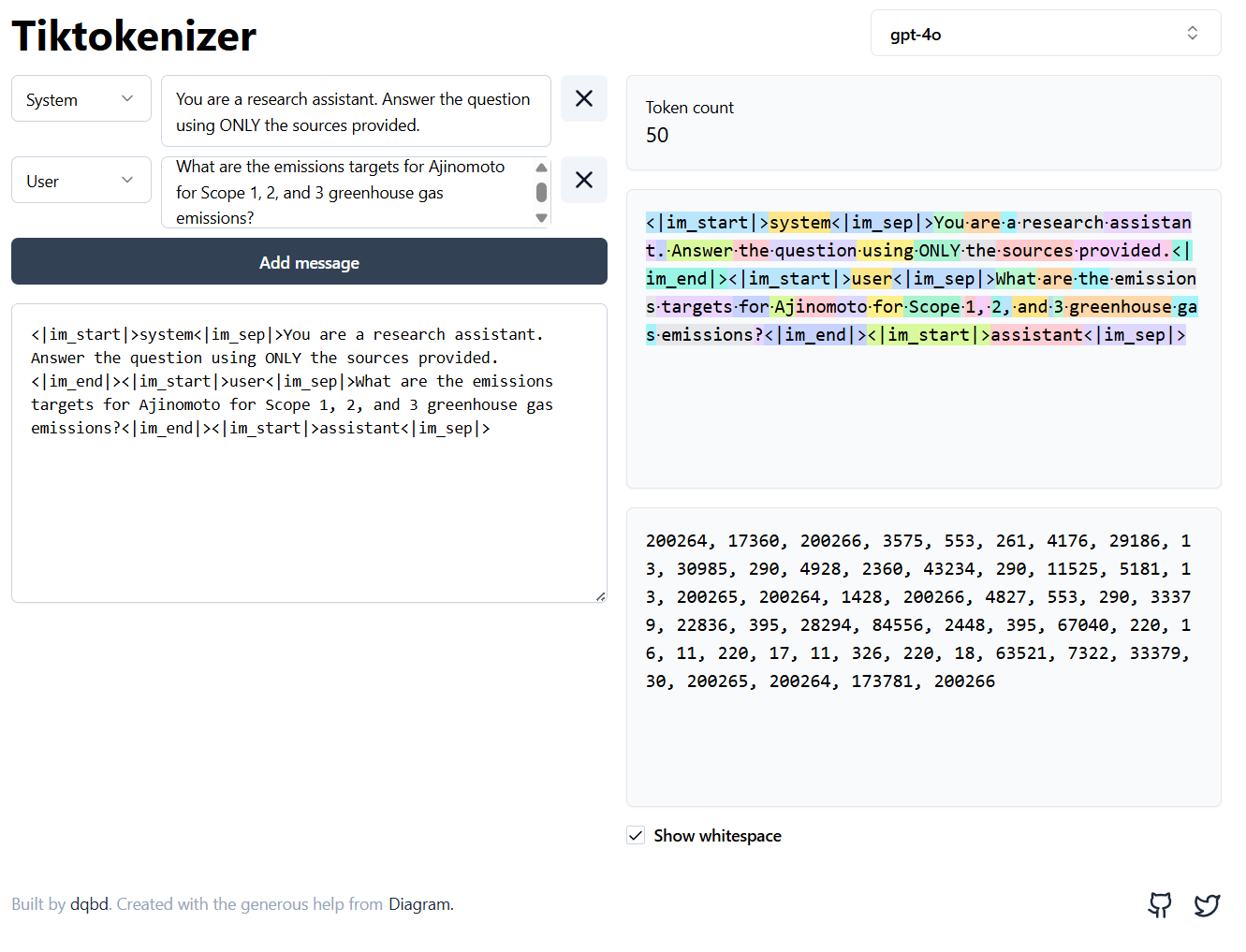
Tiktokenizer is an open-source visualiser (GitHub) that colour-codes each token so you can see the splits in real time.
Try switching between models in the dropdown. The same sentence breaks into different pieces depending on the model’s vocabulary.
This is particularly useful when debugging token budgets: paste your full prompt into the box and check whether it fits the context window before running anything.
Tool: tiktokenizer.vercel.app · Source: github.com/dqbd/tiktokenizer
How does the tokeniser learn those splits?
The dominant algorithm behind subword tokenisers is Byte-Pair Encoding (BPE). The idea in four steps:
- Start with characters. The vocabulary is every byte (or Unicode character) that appears in the training data.
- Count pairs. Scan the corpus and find the most frequent pair of adjacent tokens. Suppose
e+mappears 50,000 times. - Merge that pair. Create a new token
emand replace every occurrence ofemwithem. The vocabulary grows by one. - Repeat. Count pairs again on the updated corpus, merge the top pair, and keep going until the vocabulary reaches a target size (32,000 for TinyLlama).
After enough merges, common words like “the” become single tokens while rare words like “Ajinomoto” get split into subword pieces (Aj + ino + moto). The vocabulary size is a design choice made at training time. Once fixed, the tokeniser applies the same merge rules to any new text it sees.
BPE vs the tokeniser on your screen
The AutoTokenizer from HuggingFace does not run BPE from scratch every time. During training, BPE produces a fixed merge table (tens of thousands of merge rules in order). At inference time, the tokeniser just looks up merges in that table.
So when you call tok.encode("emissions") and get two token IDs, what happened is:
- The tokeniser checked its merge table
- Applied merges greedily, left to right
- Returned the IDs for the resulting pieces
The BPE training step happened once, months before you downloaded the model.
Not all models use BPE. The main families:
| Algorithm | Used by |
|---|---|
| BPE | GPT-2, GPT-4, LLaMA, TinyLlama |
| WordPiece | BERT, DistilBERT |
| Unigram (SentencePiece) | T5, Flan-T5, XLNet |
They differ in how they pick merges during training, but the result is the same: a fixed vocabulary of subword tokens and a deterministic encoding procedure.
The Tiktokenizer app uses OpenAI’s tiktoken library (BPE). When you switch to a BERT model in HuggingFace, you get WordPiece splits instead.
Deep dive: Andrej Karpathy, Let’s build the GPT Tokenizer (2h 13min, builds BPE from scratch in Python)
Neural Networks
A neural network is a function that takes numbers in and produces numbers out. The simplest version is a multi-layer perceptron (MLP): layers of nodes where each node computes a weighted sum of its inputs, adds a bias, and passes the result through an activation function.
Neural Networks: the building blocks
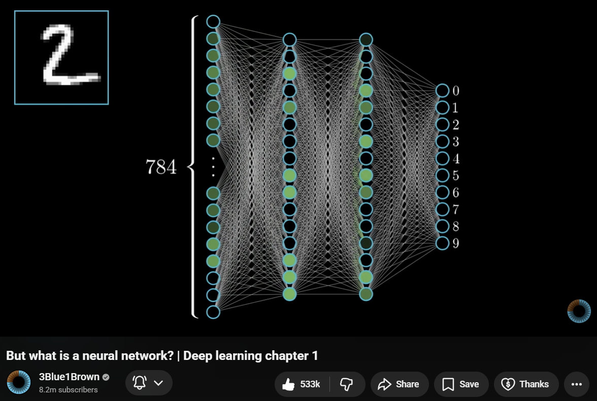
Each connection has a weight (a number the model learned during training). Training means adjusting these weights so the output gets closer to the correct answer.
For language models, the input is token IDs (as numbers) and the output is a probability distribution over the vocabulary: which token is most likely to come next?
Visual source: 3Blue1Brown, Neural Networks Chapter 1
What training looks like
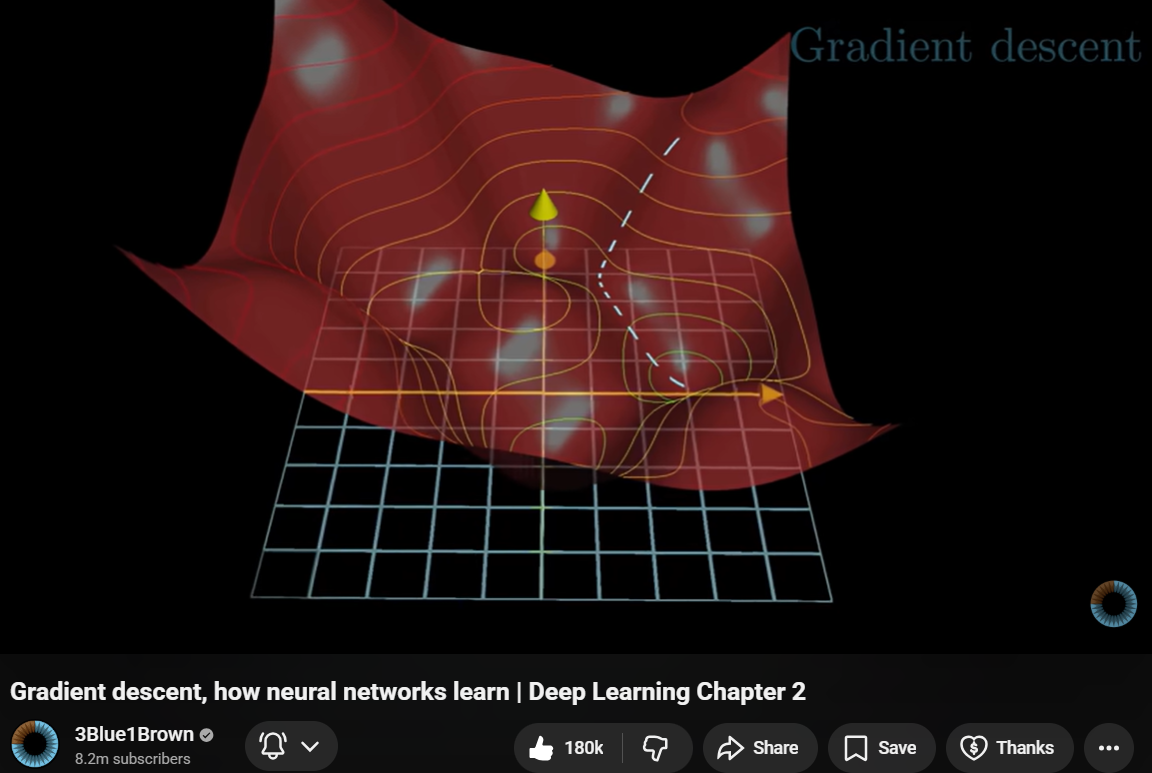
- Feed training data through the network
- Measure how wrong the output is (the loss)
- Adjust the weights to reduce the loss
- Repeat millions of times
We do not train models in this course. We use pre-trained models that someone else already trained on large datasets. Our job is to pick the right model and give it good input.
Visual source: 3Blue1Brown, Neural Networks Chapter 2
The Transformer
The transformer is the architecture behind every language model you will use in PS2. Introduced in 2017, it replaced older sequence models (RNNs, LSTMs) because it can read all tokens at once instead of one at a time.
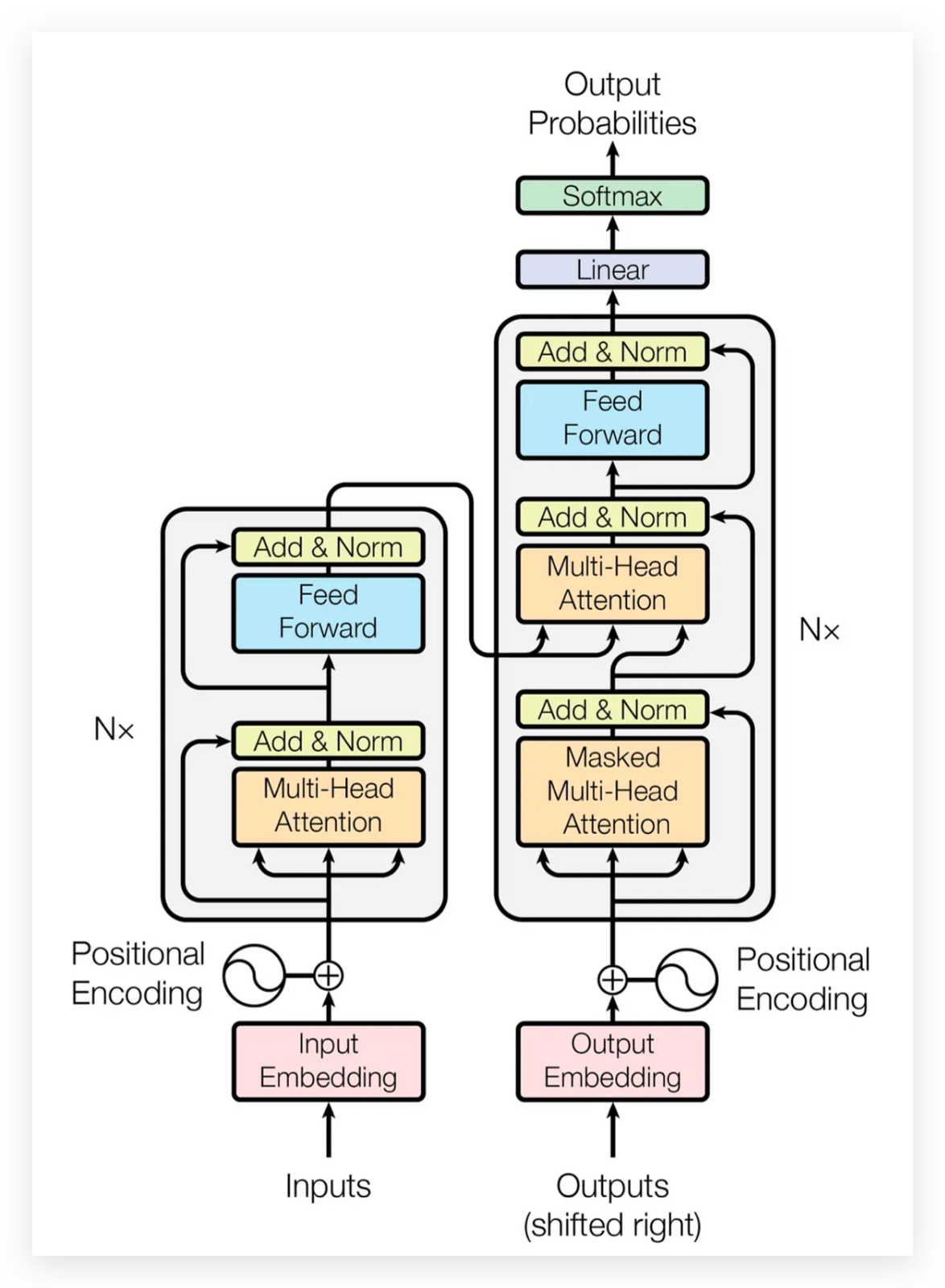
First: Encoder-Decoder architecture
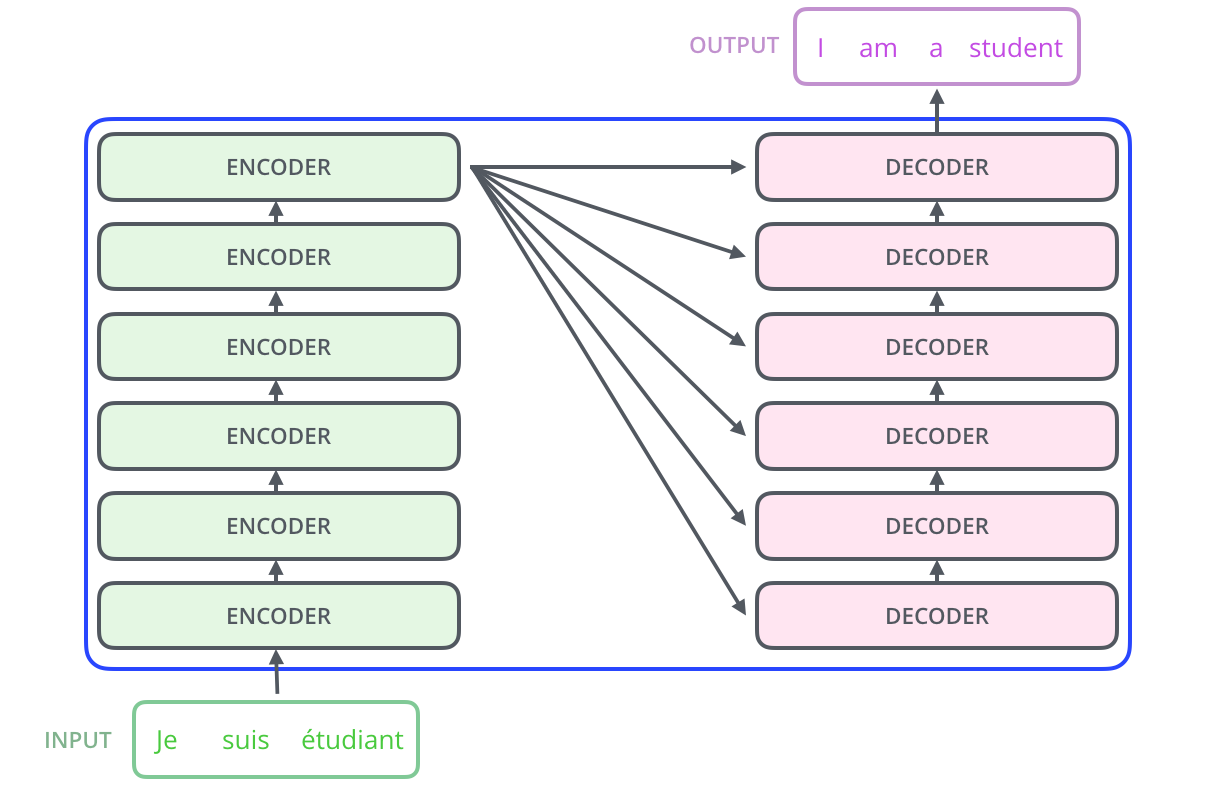
Source: Vaswani et al. 2017, Attention Is All You Need. Visual walkthrough: Jay Alammar, The Illustrated Transformer
Attention in one picture
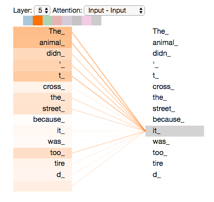
Each word produces a query (“what am I looking for?”), a key (“what do I contain?”), and a value (“what do I contribute?”). The attention score between two words is the dot product of query and key. High score means “pay attention to this word when encoding that word.”
Uses
We can use the transformer architecture in different ways depending on the task. The main families are encoder-only, encoder-decoder, and decoder-only.
Encoder-only
Reads the whole input. Produces a representation.
BERT, RoBERTa, sentence-transformers
Good for: classification, similarity, extracting spans from text.
Encoder-decoder
Reads the input, then generates output token by token.
T5, Flan-T5, BART
Good for: translation, summarisation, instruction-following.
Decoder-only
Generates text one token at a time, left to right.
GPT, LLaMA, TinyLlama, Mistral
Good for: text generation, chat, question answering.
Your embedding models from W08-W09 are encoder-only (sentence-transformers wraps BERT). The generation model in your notebook today is decoder-only (TinyLlama wraps LLaMA).
Which architecture for which task?
| Task in your pipeline | Architecture | Example model |
|---|---|---|
| Embedding chunks for retrieval | Encoder-only | all-MiniLM-L6-v2 |
| Embedding queries for retrieval | Encoder-only | multi-qa-MiniLM-L6-cos-v1 |
| Reranking retrieved chunks | Cross-encoder | ms-marco-MiniLM-L-6-v2 |
| Generating an answer from chunks | Decoder-only | TinyLlama-1.1B-Chat |
| Generating an answer from chunks | Encoder-decoder | Flan-T5-Large |
For PS2, you pick one generation model. Check the model card for its architecture, context window, and what data it was trained on.
The HuggingFace pipeline API
The pipeline function wraps model loading, tokenisation, inference, and output formatting in one call.
from transformers import pipeline as hf_pipeline

generator = hf_pipeline(
    "text-generation",
    model="TinyLlama/TinyLlama-1.1B-Chat-v1.0",
    max_new_tokens=256,
    return_full_text=False,
    do_sample=False,
    device=0,            # GPU (use -1 for CPU)
)

output = generator("What are Ajinomoto's emissions targets?")
print(output[0]["generated_text"])
On Nuvolos, omit device=0 (no GPU available). On your own machine with an NVIDIA GPU, device=0 uses CUDA.
Reference: HuggingFace pipeline tutorial
Key generation parameters
| Parameter | What it does | Recommended for PS2 |
|---|---|---|
max_new_tokens |
Maximum tokens the model will generate | 128-256 |
do_sample |
If False, always pick the most likely token (deterministic) |
False |
temperature |
Controls randomness. 0 = deterministic, higher = more varied | Only if do_sample=True |
top_p |
Limits token choices to the most probable set (nucleus sampling) | Only if do_sample=True |
return_full_text |
If False, the output contains only the new text, not the prompt |
False |
device |
-1 for CPU, 0 for first GPU |
Depends on hardware |
For PS2 evaluation: use do_sample=False so your results are reproducible. Same input always gives the same output.
Reference: HuggingFace generation strategies
Chat templates
TinyLlama (and most chat models) expect a specific format with system, user, and assistant turns marked by special tokens. If you send raw text, the model produces garbage.
from transformers import AutoTokenizer

tok = AutoTokenizer.from_pretrained(
    "TinyLlama/TinyLlama-1.1B-Chat-v1.0"
)

messages = [
    {"role": "system", "content": "You are a..."},
    {"role": "user", "content": "What are..."},
]

prompt = tok.apply_chat_template(
    messages,
    tokenize=False,
    add_generation_prompt=True,
)
The output looks like:
<|system|>
You are a...</s>
<|user|>
What are...</s>
<|assistant|>
The <|assistant|> tag at the end tells the model “now it’s your turn to speak.” Without it, the model does not know where to start generating.
Reference: HuggingFace chat templates
Adding citations to RAG
NotebookLM, Perplexity, and similar tools follow the same pattern: number the source passages in the prompt, then ask the model to reference those numbers in its answer.
The system message tells the model:
“For each claim in your answer, cite the source number in square brackets, e.g. [Source 1].”
After generation, we always append the full source list with chunk IDs, filenames, and page numbers. The reader can verify any claim.
Small models are unreliable at citing inline. The appended source list is your safety net.
Saving intermediate results with pickle
Extracting elements from a 157-page PDF with partition_pdf takes about 20 minutes. Running that every time you restart a notebook is painful. Python’s pickle module serialises any Python object to a binary file, so you can save once and reload in seconds.
When to use pickle:
- Caching expensive computations (PDF extraction, embeddings)
- Preserving exact Python objects between kernel restarts
Watch out:
- Pickle files are binary, not human-readable
- Loading a pickle from an untrusted source can execute arbitrary code
- Add
*.pklto.gitignore(they are large and not diffable)
Our CLI pipeline uses pickle as the handoff between 00_extract.py (slow extraction) and 01_chunk_strategies.py (fast chunking). You only run extraction once.
How to work with ChromaDB
In W09, we stored our chunk embeddings in ChromaDB and queried them for the first time. This section covers what ChromaDB is, how it stores data on disk, and the operations you need for PS2.
ChromaDB is an open-source vector database: it stores text, metadata, and embedding vectors together, then lets you find the nearest neighbours to a query vector in milliseconds. That nearest-neighbour lookup is the retrieve step in our RAG pipeline.
PDF → extract → chunk → embed → store (ChromaDB) → retrieve → generateChromaDB docs: trychroma.com/docs · Cookbook: cookbook.chromadb.dev · Source: github.com/chroma-core/chroma
ChromaDB vs SQLite
You already know SQLite from earlier in the course: a relational database stored in a single file, queried with SQL. ChromaDB actually uses SQLite internally for metadata and document storage, but wraps it with a vector index (HNSW) that makes similarity search fast.
| SQLite | ChromaDB | |
|---|---|---|
| Data model | Tables, rows, columns | Collections of documents + embeddings |
| Query language | SQL | Python API |
| Lookup style | Exact match, range, JOIN | Nearest-neighbour by vector similarity |
| Good for | Structured data, filtering | Semantic search over unstructured text |
| Storage | Single .db / .sqlite3 file |
chroma.sqlite3 + per-collection HNSW index folders |
ChromaDB stores its data under the directory you give PersistentClient:
data/chromadb/
├── chroma.sqlite3       ← metadata, docs, WAL
├── 2a8f1d3e-...         ← HNSW index (collection 1)
│   ├── header.bin
│   ├── data_level0.bin
│   ├── link_lists.bin
│   └── length.bin
└── 7c0e5a9b-...         ← HNSW index (collection 2)
The .sqlite3 file contains the metadata, documents, and a write-ahead log. Each collection’s embedding index lives in its own UUID-named subfolder (Chroma Cookbook, “Storage Layout”).
Try it yourself: install the SQLite Viewer extension in VS Code, then open data/chromadb/chroma.sqlite3. Browse the collections table to see your collection names and the embeddings table to see the stored chunks.
Creating and connecting to a database
ChromaDB has two client modes. For notebooks and scripts, use the persistent client so data survives kernel restarts.
Reference: Chroma Clients
Collections: create, list, delete
A collection is ChromaDB’s equivalent of a table. Each collection stores documents, metadata, and embedding vectors under a single name.
The hnsw:space parameter controls the distance metric. Use "cosine" when your embeddings are normalised (as SentenceTransformer gives you with normalize_embeddings=True). The alternatives are "l2" (Euclidean) and "ip" (inner product).
Adding documents
Every document needs a unique string ID. You can supply your own embeddings or let ChromaDB compute them.
upsertinserts new entries and overwrites existing ones with the same ID. If you useaddinstead, duplicates raise an error.- Metadata values must be strings, ints, floats, or bools. Store lists as JSON strings:
json.dumps([1,2]). - For large collections, split into batches of a few hundred to keep memory predictable.
collection.count()tells you how many documents are stored.
Querying: finding similar chunks
The core operation: embed your question, then ask ChromaDB for the k nearest vectors.
Common pitfalls:
- The outer list.
results["ids"]is a list of lists (one per query). A single query still needs[0]. - Distance vs similarity. With cosine space, distance = 1 - similarity. Smaller distance = more similar.
- Mismatched metric. If you embed with
normalize_embeddings=Truebut create the collection with the defaultl2space, distances will not match the cosine similarity you expect. Sethnsw:spaceexplicitly.
Filtering with metadata
You can narrow a query to documents that match certain metadata conditions. This is useful when you store multiple chunking strategies in the same collection, or want to restrict retrieval to specific pages.
# Simple equality
results = collection.query(
    query_embeddings=[query_vector], n_results=5,
    where={"strategy": "table_prose"},
)

# Comparison operators: $eq, $ne, $gt, $gte, $lt, $lte, $in, $nin
results = collection.query(
    query_embeddings=[query_vector], n_results=5,
    where={"char_count": {"$gte": 200}},
)

# Combine with $and / $or
results = collection.query(
    query_embeddings=[query_vector], n_results=5,
    where={"$and": [{"strategy": "table_prose"}, {"char_count": {"$gte": 200}}]},
)
Reference: ChromaDB Querying · ChromaDB Filtering
Fetching by ID and counting
Two more operations you will use frequently:
Get specific documents by ID
Use this to inspect reference chunks during evaluation, or to pull the full text for a chunk after a query returns its ID.
See the ChromaDB cookbook guide for more examples and a retrieval evaluation loop.
Reranking: a second opinion on relevance
Cosine similarity between independent embeddings is fast but rough. The bi-encoder never sees the query and the passage together, so it can miss nuance.
A cross-encoder reads the query and each candidate passage as a single concatenated input, with full transformer attention across both. It outputs a relevance score rather than an embedding.
query + all chunks → bi-encoder (fast)  → top-20 candidates
query + top-20     → cross-encoder (slow, accurate) → top-5 final
The cross-encoder is too expensive to run over thousands of chunks, so we use it only as a second stage on a shortlist from the bi-encoder.
Bi-encoder vs cross-encoder
Bi-encoder (e.g. MiniLM)
- Encodes query and document separately
- Produces one embedding per text
- Similarity = cosine between two vectors
- Fast: encode once, compare millions
- Trained with contrastive learning (positive/negative pairs)
Cross-encoder (e.g. ms-marco-MiniLM)
- Encodes query and document as one input
- Produces a single relevance score (not an embedding)
- Full attention across both texts
- Slow: one forward pass per (query, document) pair
- Trained on human relevance judgements (MS MARCO: 500k+ Bing queries)
Both use a transformer encoder, but the cross-encoder sees the interaction between query words and document words. That is why it scores relevance more accurately.
Two-stage retrieval in code
from sentence_transformers import CrossEncoder

cross_encoder = CrossEncoder("cross-encoder/ms-marco-MiniLM-L-6-v2")

# Stage 1: bi-encoder retrieves top-20
q_vec = embedding_model.encode(query, normalize_embeddings=True).tolist()
candidates = collection.query(query_embeddings=[q_vec], n_results=20)

# Stage 2: cross-encoder rescores each candidate
pairs = [(query, doc) for doc in candidates["documents"][0]]
scores = cross_encoder.predict(pairs)

# Sort by cross-encoder score and take top-5
ranked = sorted(
    zip(candidates["ids"][0], candidates["documents"][0], scores),
    key=lambda x: x[2], reverse=True,
)[:5]
No new dependencies needed. sentence-transformers already includes the CrossEncoder class.
When to add reranking
| Situation | Add reranking? |
|---|---|
| Recall@5 is low but top-20 contains the right chunks | Yes: the bi-encoder found them but ranked them too low |
| Recall@20 is also low | No: the problem is upstream (chunking or embedding model) |
| Retrieval is already good (Recall@5 near 1.0) | Probably not: little room to improve |
| Latency matters and your collection is small | Maybe not: the bi-encoder alone may be accurate enough |
For PS2, run your evaluation with and without reranking. If it helps, keep it and report the delta.
Live notebook demo
W10-NB01: From Retrieval to Generation
We will walk through the full pipeline on the Ajinomoto PDF:
1. Load the best collection from NB00 (char_limit + cross-encoder reranking)
2. Two-stage retrieval: bi-encoder top-50 → cross-encoder top-10
3. Compute token budget for Qwen2.5-1.5B-Instruct (32k context window)
4. Build prompt with numbered sources and chat template
5. Run the model, get an answer with citations
6. Fact check: did the model quote the correct numbers?
Checking the answer
Two failure modes in a RAG pipeline:
Retrieval problem
The right chunks were not retrieved. The model never saw the answer.
Measured by: Recall@5 (from W09)
Fix: change chunking, embedding model, or query.
Generation problem
The right chunks were retrieved but the model produced a wrong or incomplete answer.
Measured by: fact checking against known targets
Fix: change the prompt, try a different model, or use fewer chunks.
The diagnosis workflow
For each driving question:
| Step | What to check | How |
|---|---|---|
| 1 | Did retrieval find the right chunks? | Recall@5 against your reference set |
| 2 | Do those chunks contain the answer? | Read them manually |
| 3 | Does the model’s answer contain the correct facts? | Substring matching against expected values |
| 4 | If facts are in chunks but not in answer | Generation problem |
| 5 | If facts are not in any chunk | Retrieval problem |
You built reference sets in W09. Now you extend the evaluation to cover the generation step.
Notebook results
From the demo on the Ajinomoto PDF with Qwen2.5-1.5B-Instruct and cross-encoder reranking:
| Fact | In answer? |
|---|---|
| 50.4% | (live) |
| 30% | (live) |
| 2030 | (live) |
| 2018 | (live) |
We will fill this in from the live notebook run. The key comparison: with reranking and a 32k context window, does the model now get the facts that TinyLlama missed?
If not, check whether the facts were in the retrieved chunks. If they were but the model still missed them, that is a generation problem. If they were not, it is a retrieval problem.
Qwen2.5-1.5B runs on a laptop GPU in float16. TinyLlama (shown in the concept slides) runs on CPU in about 30 seconds. Either works for PS2.
Prompt engineering matters
The same model, the same chunks, but a different system message:
v1 (minimal)
You are a research assistant. Answer the question using ONLY the sources provided. Cite the source number in square brackets.
The model rounds numbers, invents figures, and forgets to cite per-claim.
v2 (stricter)
Rules: 1. Quote all numbers, percentages, and years EXACTLY. 2. Cite after each claim. 3. If the sources mention a topic but lack the figure, say so. 4. Numbered list, one claim per line.
The model has less room to improvise. Each constraint reduces the space of acceptable outputs.
With TinyLlama’s 2048-token window, a longer system message eats into your chunk budget. With Qwen2.5’s 32k window, the trade-off is much less painful, but it still exists.
You don’t need to chunk everything
The Ajinomoto PDF is 157 pages. The emissions targets live on a handful of them. Most pages are irrelevant to any given query.
Strategy: scan pages with a fast tool (regex on raw text, PyMuPDF) and only parse the relevant subset.
- Fewer chunks means less noise in retrieval.
- Fewer embeddings means faster indexing.
- The retriever sees only relevant material, so Recall@5 goes up.
For PS2: if your PDF is large, consider filtering pages by keyword before running partition_pdf. You already know how to write regex filters from W09.
Extractive-style prompting
Instead of generating new text, ask the same model to quote verbatim from the source chunks without paraphrasing.
No second model needed. The system message tells the model to copy the exact substring that answers the question and nothing else.
Small models may still paraphrase despite the instruction. Comparing the “quote only” answer against the generative answer tells you whether generation added value or just introduced noise.
SYSTEM_MESSAGE_EXTRACT = (
    "You are a text extraction tool. "
    "For each source, copy the EXACT "
    "substring that answers the question. "
    "Do not paraphrase, summarise, "
    "or add any words of your own.\n\n"
    "Format:\n"
    "- [Source N]: \"<exact quote>\"\n\n"
    "If a source does not contain relevant "
    "information, write:\n"
    "- [Source N]: No relevant text."
)
For true span extraction with confidence scores, see dedicated extractive QA models: HuggingFace QA task · SQuAD paper
Extractive-style vs Generative
| Dimension | Extractive-style prompt | Generative prompt |
|---|---|---|
| Hallucination risk | Lower (told to quote verbatim) | Higher (model writes new text) |
| Multi-chunk synthesis | No (one quote per source) | Yes |
| Answer naturalness | Raw substring | Fluent text |
| Extra model needed | No (same LLM) | No (same LLM) |
| Compliance | Imperfect with small models | N/A |
| Best for | Exact lookups, verifying chunk content | Synthesis across sources |
For guaranteed span extraction, dedicated encoder-only models (RoBERTa on SQuAD) predict start/end positions with confidence scores but require a separate pipeline (Lewis et al. 2020).
Honest Assessment
Small models struggle with precision. Reranking helps retrieval, but a 1.5B model still has limits.
For PS2, I care about what you tried and how you measured it. A pipeline with wrong answers and a clear diagnosis of why is better than correct answers you cannot explain.
Show your Recall@5, your fact checks, and your diagnosis table. Document what you changed between runs.
Before Thursday
Your PS2 submission needs:
| Component | What to check |
|---|---|
| Pipeline runs end-to-end | python pipeline.py run-all produces output |
| Generation step added | Retrieved chunks go into a language model, answer comes out |
| Citations attached | Each answer shows source chunk ID, PDF filename, page number |
| Evaluation documented | Recall@5 and fact checks for each driving question |
| Diagnosis table | Where did it fail? Retrieval or generation? |
| README.md | What it does, how to set up, how to run |
| CONTRIBUTING.md | How the pipeline works internally, known issues |
Resources
- Andrej Karpathy, Let’s build the GPT Tokenizer (2h 13min)
- HuggingFace tokeniser summary
- Sennrich et al. 2016, BPE for Neural Machine Translation
- HuggingFace pipeline tutorial
- HuggingFace text generation docs
- HuggingFace generation strategies
- HuggingFace chat templates
- Jay Alammar, The Illustrated Transformer
- 3Blue1Brown, Neural Networks series
- Vaswani et al. 2017, Attention Is All You Need

LSE DS205 (2025/26)