Week 09
Chunking, Embeddings, and Retrieval
DS205 – Advanced Data Manipulation
16 Mar 2026
Current State
Last week, we extracted about 15,500 text elements from a sustainability report PDF. We ranked them by embedding similarity for a naively written query. The top results were essentially just noise.
The text units were too raw, and retrieval had no grounded reference set for evaluation.
Our chunking situation
How to make the chunks more useful for retrieval system we’ll build later?
raw text elements (from unstructured)
-> chunking
-> embedding
-> some type of similarity search
-> top-k results
-> check against known answers
We will create a baseline of solutions to help us evaluate different approaches. Without something like this, we have no way of knowing if we are making progress.
Chunking: Strategy A
Let me start with the simplest possible approach: split the raw text into fixed-size chunks of about \(n_\text{fixed} \approx 1000\) characters (with a buffer to avoid splitting mid-word).
| id | text | strategy | source | char_count |
|---|---|---|---|---|
| char_0000 | Ajinomoto Group Sustainability Report 2025 Sustainability Policy and Framework Help Extend the Healthy Life Expectancy of 1 Billion People Reduce Our Environmental Impact by 50% Social Governance Contents Sustainability Policy and Framework P004 Reduce Our Environmental Impact by 50% Message from the CEO P005 Environmental management Message from the Executive Officer in Charge of Sustainability P006 Climate change […] | char_limit | SR2025en_all.pdf | 1030 |
| char_0001 | Help Extend the Healthy Life Expectancy of 1 Billion People P036 Human rights and human resources Initiatives to solve nutritional issues P037 Human rights Cooking and sharing meals P047 Human resources management Medical foods P048 Occupational safety and health Disseminating information on MSG safety and benefits P049 Supply chain management Addressing health issues P051 Strengthening relationships […] | char_limit | SR2025en_all.pdf | 1044 |
A simple custom function to do that is available in the accompanying utils.py file.
Chunking: Strategy B
Another idea is to use the structure of the document we are parsing to guide chunking. The partition function gives us a list of elements with types like “Title”, “Heading”, “Text”, “ListItem”, etc.
We can make use of that…
Chunking: Strategy B (cont.)
In this alternative strategy, we define a chunk as the piece of text between two major structural elements (Title and Header, in my example).
This way, we can preserve some of the document’s logical sections and their context, which may help retrieval later on.
I decided to add a RUNNING_TITLE and HEADER field to the chunk metadata in the hope that they would help retrieval later on. Chunking is a bit of an art sometimes 🎨🖌️
| id | text | strategy | pages | element _types |
char _count |
|
|---|---|---|---|---|---|---|
| elem_0000 | RUNNING TITLE: Ajinomoto Group Sustainability Report HEADER (H2): (no header) 2025 |
element_type | [1] | [‘Text’, ‘Title’] | 84 | |
| elem_0001 | RUNNING TITLE: Ajinomoto Group Sustainability Report HEADER (H2): Governance P004 P005 P006 Climate change (disclosures based on the |
element_type | [2] | [‘Header’, ‘NarrativeText’, ‘Text’, ‘Title’] | 497 |
A side-by-side comparison
Further down in the document, this is what a section that includes emissions targets looks like in the two strategies:
Strategy A - char_0052
FY2030: 50.4% reduction in Scope 1 and 2, 30% reduction in Scope 3 (vs. FY2018) - FY2050: Net zero, 100% renewable energy for electricity - Reduction of GHG emissions from cattle by providing solutions using specialized feed-grade amino acids…
Target content is present, but mixed with adjacent list fragments.
Strategy B - elem_0046
RUNNING TITLE: Significant
HEADER (H2): 017
FY2030: 50.4% reduction in Scope 1 and 2, 30% reduction in Scope 3 (vs. FY2018) - FY2050: Net zero, 100% renewable energy for electricity…
The heading is not all that meaningful because that chunk is actually inside a table! More on tables and chunking later.
Chunk Length Distributions
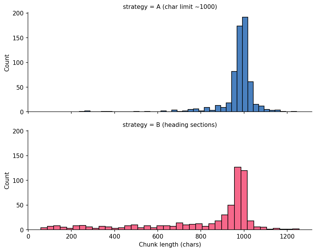
Strategy A is tightly clustered near 1000. Strategy B spreads across shorter and longer section-driven chunks.
More Promising Approaches
Those can be easily replicated from the official documentation of langchain-text-splitters and unstructured. I have not tested those on Nuvolos though!
LangChain splitter choices
Check out the official documentation for LangChain text splitters for more options and details on how they work. The recursive splitter is a good general-purpose choice that tries to split on natural boundaries first (e.g. paragraphs, sentences) before falling back to character limits.
unstructured for PDF tables
hi_res + table inference can preserve table structure so you can summarise table content for retrieval instead of losing it in flat text.
Perhaps a hybrid approach will be what work best for our use case, as we want to preserve some of the document structure but also have a more consistent way to demarcate end of paragraphs and sections.
What people in the industry are saying
Greg Kamradt, president of the ARC Prize, proposes the following chunking taxonomy which I find useful for our purposes:
| Level | Kamradt label | Our notebook |
|---|---|---|
| 1 | Fixed-size splitting | Strategy A |
| 2 | Recursive splitting | Not covered |
| 3 | Document-structure splitting | Strategy B |
| 4 | Semantic splitting | Not covered |
| 5 | Agentic splitting | Not covered |
How should we search a text corpus?
In this course, we teach you how to build a retrieval system (RAG) which is a technique that is built on top of language models*. It’s a particular way to search for relevant information and present it to a user.
Information Retrieval is a huge field with a long history, and there are many different approaches to it. But for our purposes, I will keep it constrained to just techniques that might help you with your projects.
* Remember: this doesn’t necessarily mean large language models. In fact, I want you to try out the small ones first!
Before ML: Regex
How can I do a Ctrl + F using Python to search for emissions targets with pattern matching before I run a model?
Read more about regex in Python here. There also entire books on the topic!
Effectively, the code on the left is searching the document for the presence of strings that match the patterns below. The \b means “word boundary”, so we only match whole words and not substrings.
- “Scope 1”, “Scope 2”, “Scope 3”, “Scope I”, “Scope II”, or “Scope III” (case-insensitive)
- “target”, “targets”, “goal”, “goals”, “reduce”, “reduction”, “net zero”, or “emission(s)” (case-insensitive)
Regular Expressions (cont.)
How can I do a Ctrl + F using Python to search for emissions targets with pattern matching before I run a model?
scope_pattern = (
    r"\bscope\s*(?:1|2|3|i|ii|iii)\b"
    r"|\bscope\s*1\s*and\s*2\b"
)
target_pattern = (
    r"\b(target|targets|goal|goals|"
    r"reduce|reduction|net zero|emissions?)\b"
)

# Imagine we combine those in two boolean series and
# get a final candidate
candidates = chunks_df[
    chunks_df["text"].str.contains(scope_pattern, regex=True) &
    chunks_df["text"].str.contains(target_pattern, regex=True)
]| Metric | Count |
|---|---|
| Total chunks | 578 |
| Scope mentions | 30 |
| Target language | 238 |
| Both scope + target | 23 |
Regex gets us to 23 candidate chunks quickly, but only because we already know which words to search for.
Regex Noise Filtering
Regex is precise, but not all matches are useful retrieval targets. You might want to build additional regex patterns to filter out false positives that match your target patterns but are not actually relevant to your retrieval task.
Filtered examples
- “Appendix 1: Environmental Data …”
- “Our assurance engagement covered …”
These lines are valid regex hits for target-like terms but not the target paragraph we want. Here the (?i) at the start of the pattern means “case-insensitive”, so we match words like “Appendix” or “appendix”. The \b again means “word boundary” to avoid matching substrings.
Reference Answers
These are the chunks I found manually, with the help of those regex patterns, in the PDF and will use as reference answers for retrieval checks.
| ID | Page | Contains |
|---|---|---|
| elem_0046 | 17 | “FY2030: 50.4% reduction in Scope 1 and 2, 30% reduction in Scope 3 (vs. FY2018)” |
| elem_0063 | 24 | “reduce greenhouse gas emissions in fiscal 2030 by 50.4% for Scope 1 and 2 and 24% for Scope 3” |
| elem_0208 | 62 | “Scope 1 and 2: Reduce GHG emissions by 50.4% by FY2030” |
| elem_0209 | 62 | “Scope 3: Reduce GHG emissions by 30% by FY2030” |
24% and 30% both appear because the report includes old and revised Scope 3 targets in different sections.
Tip: Regex Debugging
AI coding tools can often write good regex patterns for you, if you specify what you want to match and not match in natural language. Always try to be specific with your prompts! and consider exploring the matches on a Jupyter Notebook before enshrining them in your pipeline.
When I feel like I really want/need to understand a regex pattern, I like to use regex101 which is a great interactive regex tester and debugger. I also like the debuggex tool for visualising regex patterns as graphs.
It would be tedious to teach you regex in depth in this course but I encourage you to explore it on your own if you are interested. Take a look at this cheatsheet for example, or as mentioned before, the Python docs.
Word2Vec: a more flexible approach
Let me take you on a quick detour to show you another technique that, again, might not be as fun and exciting nowadays but that was foundational to the development of word embeddings and language models: Word2Vec.
Putting it simply, Word2Vec is a method for learning vector representations of words based on their co-occurrence patterns in a text corpus. It was introduced by Mikolov et al. in 2013 and has been widely used in NLP tasks since then.
Word2Vec Setup
As a programmer, all you need to do is install the gensim library and feed it a list of tokenised sentences. The library will take care of the rest, including training the model and generating word vectors.
For a visual walkthrough, see 3Blue1Brown on word embeddings.
What is tokenisation?
Tokenisation converts a string into a list of tokens. For Word2Vec, each token is a word.
Numbers and punctuation are stripped by simple_preprocess, which is why 50.4% does not survive as a useful token in this corpus.
This is one reason Word2Vec struggles with numerical targets in policy text.
Word2Vec Training Objectives
Word2Vec has two training modes. CBOW predicts a target word from surrounding context words. Skip-gram predicts surrounding context words from a target word.

CBOW: predict the centre word from context.

Skip-gram: predict context words from the centre word.
gensim defaults to Skip-gram when sg=1. Both methods produce the same kind of word vectors.
Diagram sources (CC BY-SA 4.0): Wikimedia Commons, “Word embeddings CBOW” and “Word embeddings Skip-gram”.
Word Similarities
The model learns useful neighbourhoods from corpus context without manual keyword lists. For example, most_similar("emissions", topn=8) on the Ajinomoto corpus:
| Word | Score |
|---|---|
| ghg | 0.922 |
| reductions | 0.895 |
| gas | 0.895 |
| greenhouse | 0.886 |
| scope | 0.849 |
Vector Arithmetic
It’s fun to see what internal relationships the model has learned by doing vector arithmetic. For example, we can try to find words that are similar to “greenhouse” and “gas” but not “renewable”:
| Equation | Top results | Reading |
|---|---|---|
greenhouse - gas + renewable |
energy (0.945), electricity (0.926) |
Renewable-energy vocabulary |
sugar + oil - palm |
cane (0.867), milk (0.850) |
Other raw materials |
water + scope - emissions |
fresh (0.828), withdrawal (0.794) |
Water measurement terms |
You should read the above like this: “greenhouse is to gas as renewable is to energy and electricity”. The model has learned that “greenhouse” and “gas” are related, and that “renewable” is related to “energy” and “electricity”, so it can make the analogy.
UMAP Projection
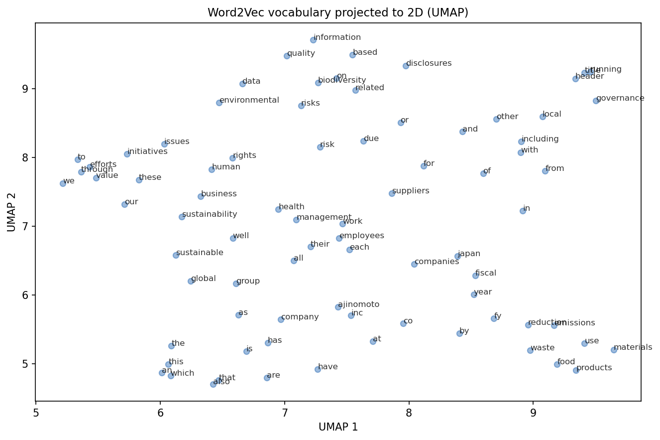
The so-called stopwords dominate frequency. Domain terms form tighter local regions on the right side.
How similarity is computed
Because each word is represented as a vector, we can compute similarities between words and use that for retrieval. For example, we can compute the cosine similarity between the vector for “emissions” and the vectors for each chunk to find the most relevant chunks.

\[ \cos(\theta)=\frac{A\cdot B}{\|A\|\times\|B\|} \]
For normalised vectors, \(\|A\|=\|B\|=1\), so cosine similarity is the dot product: \(\cos(\theta)=A\cdot B\).
This is what np.dot(unit_vecs, query_vec) computes in the notebook. Each retrieval score is a cosine similarity.
Working with several words
When we want to compute similarity between a query and a chunk, we can average the vectors of the individual words in the query and the chunk to get a single vector representation for each. Then we can compute the cosine similarity between those two vectors.
This is unlikely to work though… do you see why?
Strategy A top-5
| Rank | Chunk ID | Score |
|---|---|---|
| 1 | char_0232 | 0.941 |
| 2 | char_0235 | 0.929 |
| 3 | char_0616 | 0.926 |
| 4 | char_0569 | 0.915 |
| 5 | char_0584 | 0.905 |
Strategy B top-5
| Rank | Chunk ID | Score |
|---|---|---|
| 1 | elem_0217 | 0.928 |
| 2 | elem_0211 | 0.896 |
| 3 | elem_0536 | 0.892 |
| 4 | elem_0215 | 0.890 |
| 5 | elem_0214 | 0.889 |
None of those matches were in my pre-selected reference-answer set. Hits: A = 0/4, B = 0/4.
Reading The Whole Chunk
Word2Vec gives one vector per word. To get a chunk vector, we averaged word vectors which effectively dillutes the ‘signal’. (Try it out with a pre-trained Word2Vec from Gensim to see if it improve results.)
Sentence-transformers take a different approach: they read the whole chunk through a transformer network and produce one vector directly.

Transformers and BERT-based Models
BERT (Bidirectional Encoder Representations from Transformers) reads text in both directions simultaneously. It was trained on large corpora to predict masked words and recognise sentence relationships.
We use pre-trained BERT models as feature extractors: feed in a chunk of text, get back a fixed-size vector.
The internal mechanics (attention layers, positional encodings) are beyond DS205 scope. For retrieval, the key point is that BERT-based models produce context-aware vectors where each word depends on surrounding words.
Similarity Model Results
Strategy B - all-MiniLM-L6-v2
| Rank | Chunk ID | Score |
|---|---|---|
| 1 | elem_0215 | 0.652 |
| 2 | elem_0217 | 0.635 |
| 3 | elem_0212 | 0.621 |
| 4 | elem_0222 | 0.580 |
| 5 | elem_0046 | 0.564 |
elem_0046 appears at rank 5. 1/4 reference chunks in top-5.
Same Architecture, Different Training
all-MiniLM-L6-v2
Sentence similarity objective
Large mixed corpus of sentence pairs
About 1B training pairs
multi-qa-MiniLM-L6-cos-v1
Question-answer retrieval objective
Optimised for query and passage matching
About 215M question-answer pairs
Model cards: all-MiniLM-L6-v2 Model cards: multi-qa-MiniLM-L6-cos-v1
Q&A Model Results
Strategy B - multi-qa-MiniLM-L6-cos-v1
| Rank | Chunk ID | Score |
|---|---|---|
| 1 | elem_0063 | 0.693 |
| 2 | elem_0217 | 0.657 |
| 3 | elem_0215 | 0.635 |
| 4 | elem_0222 | 0.619 |
| 5 | elem_0046 | 0.605 |
elem_0063 ranks first and contains the explicit Scope 3 target statement. 2/4 reference chunks in top-5.
Strategy A Results
MiniLM Similarity A top-5
| Rank | Chunk ID | Score |
|---|---|---|
| 1 | char_0235 | 0.700 |
| 2 | char_0209 | 0.589 |
| 3 | char_0052 | 0.588 |
| 4 | char_0229 | 0.572 |
| 5 | char_0226 | 0.570 |
MiniLM Q&A A top-5
| Rank | Chunk ID | Score |
|---|---|---|
| 1 | char_0234 | 0.662 |
| 2 | char_0235 | 0.649 |
| 3 | char_0052 | 0.624 |
| 4 | char_0204 | 0.622 |
| 5 | char_0233 | 0.590 |
Strategy A hits: MiniLM Similarity A = 2/4, MiniLM Q&A A = 1/4.
Under The Hood
from transformers import AutoTokenizer, AutoModel

model_name = "sentence-transformers/all-MiniLM-L6-v2"
tok = AutoTokenizer.from_pretrained(model_name)
mdl = AutoModel.from_pretrained(model_name)
batch = tok(texts, padding=True, truncation=True, return_tensors="pt")
out = mdl(**batch).last_hidden_state
mask = batch["attention_mask"].unsqueeze(-1)
emb = (out * mask).sum(dim=1) / mask.sum(dim=1).clamp(min=1)
SentenceTransformer wraps this tokenisation, encoding, and pooling path.
Full Comparison
| Method | Recall@5 | Hits | Total |
|---|---|---|---|
| Word2Vec A (trained on small corpus though) | 0.00 | 0 | 4 |
| Word2Vec B (trained on small corpus though) | 0.00 | 0 | 4 |
| MiniLM Sim A | 0.50 | 2 | 4 |
| MiniLM Sim B | 0.25 | 1 | 4 |
| MiniLM QA A | 0.25 | 1 | 4 |
| MiniLM QA B | 0.50 | 2 | 4 |
Two configurations tied at 0.50. Neither chunking strategy dominated across all models. Neither model dominates across all strategies.
Recall at k: fraction of relevant documents retrieved in the top k results.
Honest Assessment
Best Recall@5 is 50%. Half the target chunks are still missing.
For PS2, I care about what you tried and how you measured it. Document your configurations, show recall numbers, and explain what changed between runs.
A lower score with a clear method is better than a higher score you cannot explain.
Choosing A Model
Use the MTEB leaderboard.
- Filter by Retrieval
- Check language/task fit before score rank
- On Nuvolos, keep model size practical for your compute budget
Tomorrow In Lab
Store embeddings in ChromaDB so they persist between sessions and support metadata filtering. Notebook: W09-NB02.
Challenge Directions
This is what the groups working on RAG projects for their final projects discovered by searching the web for relevant papers and blog posts. You can use these as inspiration for your own project research, but they are absolutely NOT required to read or implement any of these methods for PS2.
| Direction | Reference |
|---|---|
| ClimateBERT comparisons | Webersinke et al. 2022 |
| Hybrid BM25 + semantic retrieval | Gao et al. 2022 |
| HyDE query seeding | Gao et al. 2022 |
| HopRAG traversal | Fan et al. 2025 |
Resources
- W09-NB01 lecture notebook
- Mikolov et al. 2013, Efficient Estimation of Word Representations in Vector Space
- Reimers and Gurevych 2019, Sentence-BERT
- MS MARCO dataset paper
- Stanford IR textbook, evaluation of ranked retrieval
- all-MiniLM-L6-v2 model card
- multi-qa-MiniLM-L6-cos-v1 model card
- Greg Kamradt 5 levels of text splitting
- 3Blue1Brown word embeddings visual walkthrough
- Sentence Transformers docs
- Unstructured partitioning docs

LSE DS205 (2025/26)