🗣️ Week 08: From Word Vectors to Transformers
DS205: Advanced Data Manipulation
10 Mar 2025
Hour 1: Neural Foundations of Transformer Models
Introduction & Outline
Introduction & Outline
Biological inspiration
1. Anatomy & PhysiologyComputation & learning computations
2. Functional mapping
3. Prediction
4. Matrix mutliplication
5. Errors - landscape
6. Gradients
7. Training lifecycle
Deep Learning
8. Multi Layered Perceptrons: Stacking layers - abstractionCode
Data
Consequences
Questions
Biological Inspiration
Biological Inspiration
- Neural networks inspired by brain structure
- Neurons, synapses, and signal transmission
- From biological neurons to artificial neurons
Anatomy & Physiology
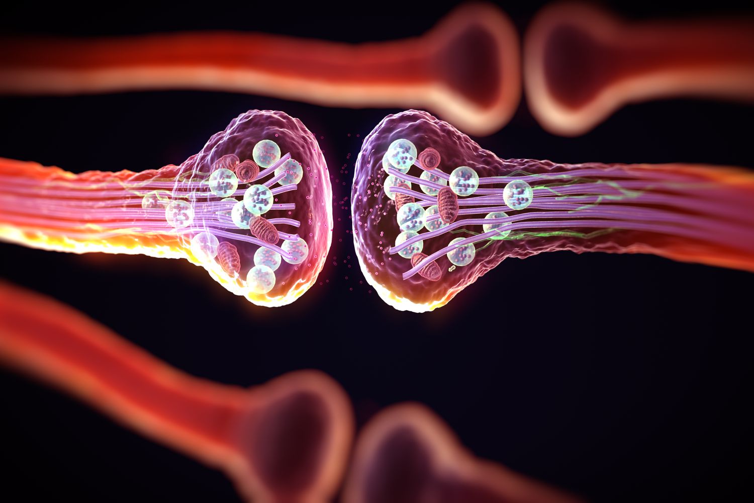
- Cortical tissue – although there are also input stages
- Networks of neurones
- Layered – ~6 layers within cortex
- Axons – electrical transmission (via action potentials, a.k.a. “spikes”)
- Synapses
- “Gap junction” – chemical transmission
- “Weights” == “propensity/sensitivity to absorb the neurotransmitter”
- Synapses
Anatomy & Physiology
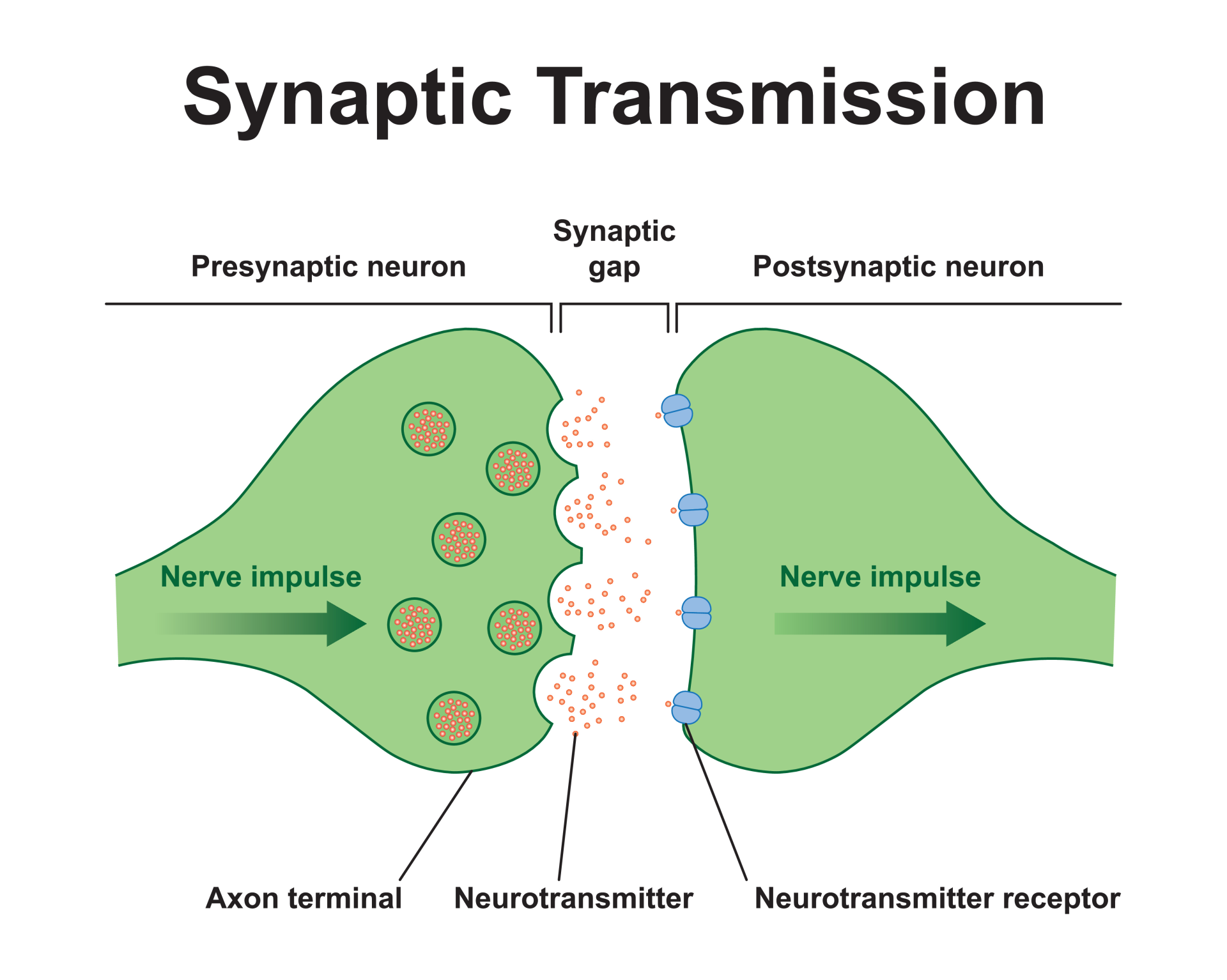
- Hebbian Leaning
- Sensitivity increases when neurones fire jointly
- i.e. When they are simultaneously active
- Sensitivity increases when neurones fire jointly
Learning
Computation & Learning Computations
Functional mapping:
Linear: A straight line is a model
- Basic – scaling, shifting, rotation without deformation
- It has 2 parameters:
- We can know what these are (from prior knowledge and understanding), or …
- We can search for them
\[ \color{#a8f} {y = wx + b} \]
\(w\) is the slope \(\rightarrow\) i.e. one of these means “one-dimensional”
\(b\) is the bias (offset) \(\rightarrow\) everpresent output, no matter what you do
- This “model” can be used for classification or regression
- It is also at the root of all, much more powerful, non-linear models
Functional mapping:
High-dimensional “spaces” – a pillar of neural computation
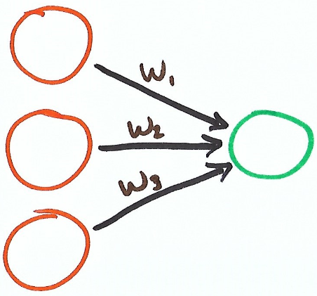
\[ \color{#a8f} {y = w_{1}x_{1} + w_{2}x_{2} + ... + b} \]
- For more complex situations, we just add extra “levers” – or, parameters \(w_{i}\)
- This is now multi-dimensional .. but now we have to search by moving two.. or three, or four, .. or … \(n\) levers at a time
Prediction
MLP: 2 modes of prediction …
- Regression problems
- “Here is our input, what is the value of our output?”
- Classification problems
- “Here is our input, we estimate our output. Which class does this fall into?”
NLP: language (sequence) modelling – “semi-supervised learning”
- From word vectors to contextual understanding
Matrix multiplication

Networks of neurones become matrices – used for matrix x vector multiplication
- The mathematical foundation
- Efficient parallel computation
- Scaling to large language models
Non-linear relationships
Any relationship that isn’t linear!
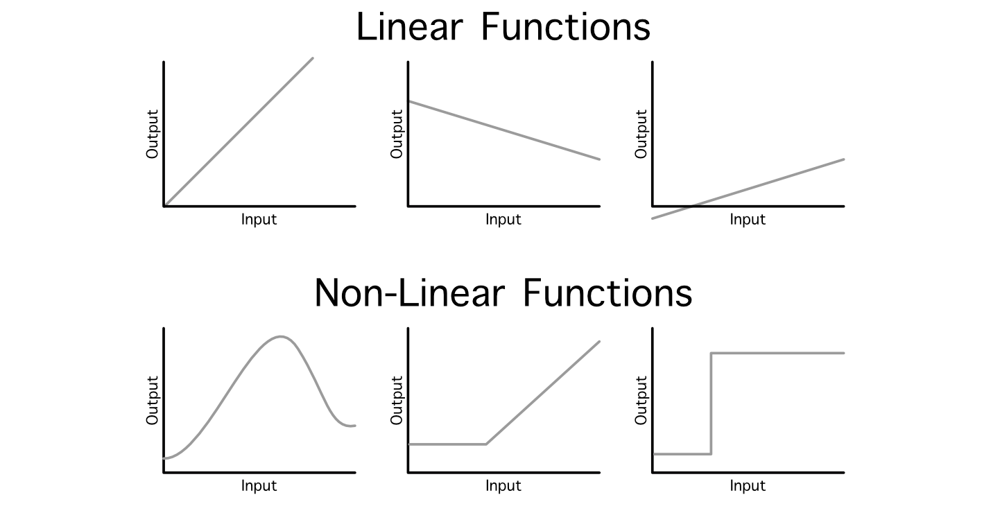
The whole modelling paradigm becomes much more powerful when the relationships we model are no longer described by simple linear rules
The non-linearity is the essential catalyst and all-imporant ingredient!
\[ \color{#a8f} {y = sin(x)} \]
\[ \color{#a8f} {y = w_{1}. exp(x_{1}) + w_{2}.cos(x_{2})} \]
\[ \color{#a8f} {y = x^{2} + x^{3} + x^{4}} \]
\[ \color{#a8f} {\vdots} \]
\[ \color{#a8f} {\text{everything else!}} \]
This can render analysis quite intractable

Representation
“Models” are “blocks of numbers”!
- “Neural network models” are “blocks of numbers”! – i.e. not code
- You could store these numbers within any suitable substrate
- We store them in memory (RAM) and as files (on disk) – today!
- Diffuse representations a.k.a. parallel distributed – “connectionist”
- You could store these numbers within any suitable substrate
Diffuse representations a.k.a. parallel distributed network – a.k.a. “connectionist”
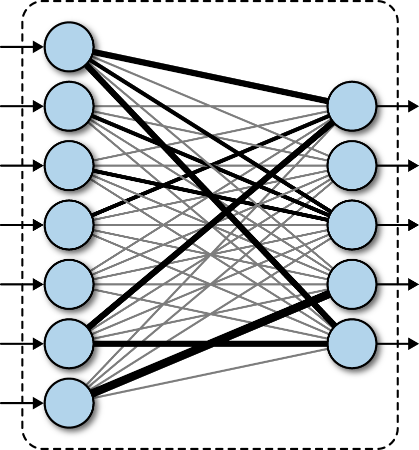
- These numbers are the “firing rates”
- Numbers/weights/parameters are discrete, but the representation is distributed
- If each number is the distance along an axis, then the set of numbers forms a “space” – a so called “latent space” that encodes “deeper information” – meaning?
Research in this field is all about finding “good numbers” to perform well doing “things we care about”
“Neural Networks”
a.k.a:
- Feed-Forward Neural Networks (FF)
- Fully-Connected Neural Networks (FCN)
- Artificial Neural Networks (ANN)
- Multi-Layered Perceptrons (MLP)
Learning
Learning!
Errors – Landscape
- Loss functions
- Error surfaces
- Optimization challenges
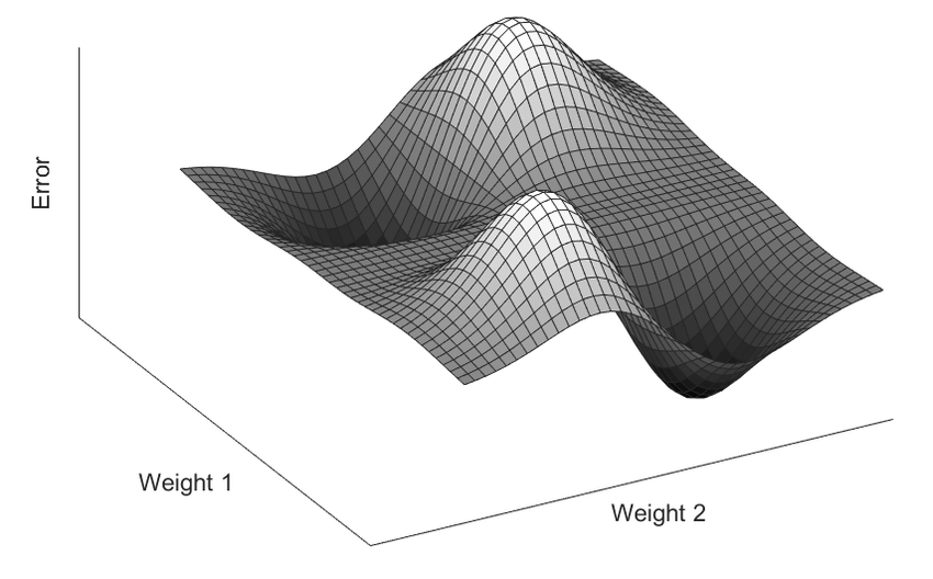
Loss
Loss Function – a.k.a. “cost function”, “error”: “Distance Measures” – our “gap”
A cost function looks like a smooth, curved line, across a graph. For any point on this line, the height above zero represents “cost” in some way – e.g. how much “energy” the model will incur when tuned to a specific setting. The higher the point, the farther from ideal (of 0) the system is. We want to find the lowest point on this line, where the cost is smallest.
Common loss functions include:
- Mean Square Error for regression tasks: \(MSE = \frac{1}{n} \sum_{i-1}^{n}(Y_i - \hat{Y}_{i})^{2}\)
- Negative Log Likelihood for classification: \(-log L(\theta|x) = - \sum{log P(x_{i}|\theta)}\)
- Cross Entropy Loss (logistic loss function) – which will normalize logits
- \(H(p, q) = -\sum_{i}p_{i}\log q_{i} = -y \log \hat{y} - (1-y)\log(1-\hat{y})\)
- Combines Log Softmax and Negative Log Likelihood
Gradients
- Partial derivatives
- Direction of steepest descent
- Learning rate considerations
Gradient descent algorithms “feel their way” to the bottom of the curve by picking a point and calculating the slope (or gradient) of the curve around it, and then moving in the direction where the slope is steepest
- Imagine this as feeling your way down a mountain in the dark. You may not know exactly where to move, or how close to valley floor you will get, but if, in general, you head down the slope in the steepest direction, you would hope to arrive at the lowest point in the area
The Chain Rule
If \(y = f(u)\) and \(u = g(x)\), then
\[ \frac{dy}{dx} = \frac{dy}{du} . \frac{du}{dx} \]
.. the “outside function” is \(f()\) and the “inside function” is \(g()\)
Chain rule translates as: “the derivate of the ‘outside’” \(\times\) “the derivative of the ‘inside’”
Alternatively,
If \(y = f[g(x)]\)
Then \(y' = f'[g(x)].g'(x)\)
Training Lifecycle
- Forward pass
- Backward pass (backpropagation)
- Weight updates – until convergence
Backpropagation
- Training hidden layers – “breaking free from Minski’s XOR cage”
Backpropagation is a gradient estimation method used to train neural network models. The gradient estimate is used by the optimization algorithm to compute the network parameter updates.
It is an efficient application of the chain rule to such networks (known since 1673). It is also known as the reverse mode of automatic differentiation.
- Automatic differentiation is a powerful software technique used to learn (any) parameter from error gradients
Deep Learning
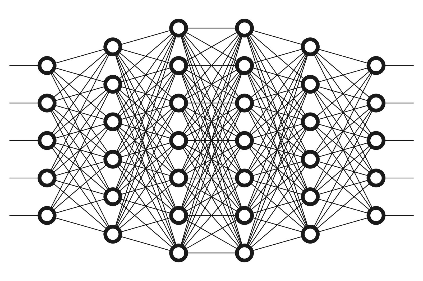
Multi-Layered Perceptrons: Stacking Layers → Abstraction
- Hidden layers and representation learning
- Automatic feature engineering
- From shallow to deep architectures
The phrase “‘’Deep Learning’’” really applies to any design of neural network that makes use of many layers – today, numbering 10s, 100s or even 1000s of layers.
The explosion of interest in Deep Learning began with the success of AlexNet in a machine vision competition (circa. 2012)
Our “latent space”, which encodes our ”deeper information”, abstracts – meaning as we penetrate deeper into the network*
- Automatic feature engineering
In the early history of neural computation, the computational power obtained by stacking multiple layers was not fully recognised, and in any case, few researchers had access to the scale of compute necessary to explore these advantages. Early neural networks used around 3-5 layers.
Transformers
- A Transformer block is an Attention layer + MLP layer
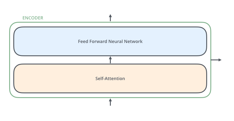
- A Transformer stacks multiple Transformer blocks”
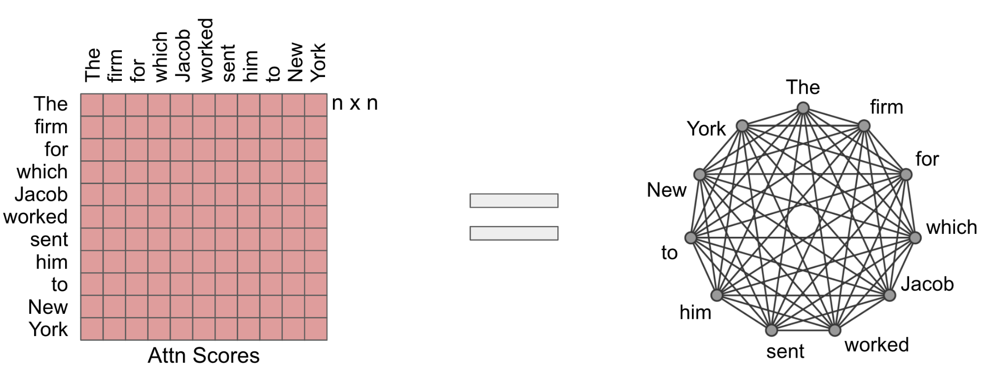
Attention

Code
- Basic neural network implementation
- Key components and functions
import numpy as np
# f = x * x -- i.e. no bias term
X = np.array([1, 2, 3, 4], dtype=np.float32)
y = np.array([2, 4, 6, 8], dtype=np.float32)
w = 0.0
# loss = MSE -- in the case of linear regression
def loss(y, y_predicted):
return ((y_predicted - y)**2).mean()# gradient
# MSE = 1/N * (w*x -2)**2
# dJ/dX = 1/N * 2x (w*x -y) -- the symbolically calculated derivative
def gradient(x, y, y_predicted):
return np.dot(2*x, y_predicted-y).mean()print(f'prediction before training: f(5) = {forward(5):.3f}')
#Training
learning_rate = 0.01
n_iters = 10
for epoch in range(n_iters):
# prediction
y_pred = forward(X)
# loss
l = loss(y, y_pred)
# gradients
dw = gradient(X, y, y_pred)
# update weights
w -= learning_rate * dw
if epoch %1 ==0:
print(f'epoch {epoch+1}: w = {w:.3f}, loss {l:.8f}')
print(f'Prediction after training: f(5) = {forward(5):.3f}')Data
Data is “anything we know how to record (and represent using a number)”
Anyone, with records of anything, can turn to machine learning
Modelling “the world” – the whole enterprise of neural network modelling aims to capture structure within data
- Records – e.g. a corporate spreadsheet, or instrument measurements
Unstructured data
- Pixels
- Sounds
- Words \(\rightarrow\) language
Intrinsically semantic data
Token sequences (and sets) – now we are interested in relations
- Proteins from DNA
- Chemistry – molecular structure
- Crime – pattern matching on motifs
The physical world
Consequences
- Neural networks work with any data – we just require a numerical form of representation
- We can learn arbitrary functions (mappings) – without having to define the complex mathematical relationships ourselves
- Deep relationships between features
- Neural networks are universal!
- An abstraction takes place as we penetrate deeper into the network
- Vision: image structure (similar to that found in early mammalian vision)
- Language: words \(\rightarrow\) “concepts” \(\rightarrow\) “meaning”?
- It appears that computational power increases with scale
- But, networks are modelled as graphs – and these imply exponential burden
- There is no “code” – inductive bias is a “dirty” idea
- Models are limited by data quality – “world models” are based on our ability to “sample the world”
Questions
- Discussion
- Clarifications
- Transition to Hour 2
Hour 2: Transformers for Climate Document Retrieval
Dr. Jon Cardoso-Silva
🖥️ Live Demo
![]()
LSE DS205 (2024/25)
