🗓️ Week 09:
Unsupervised learning II: More clustering, anomaly detection and dimensionality reduction

Theme: Unsupervised learning

Dr. Ghita Berrada

LSE Data Science Institute

2023-11-24

What we will cover today

• ⏪ Recap time: Clustering
• Another type of clustering: density-based clustering with DBSCAN
• Anomaly detection
• Dimensionality reduction
• What’s next?

⏪ Recap time: Clustering

• Clustering is an unsupervised learning technique
• Its goal is to group together “similar” data points in the dataset and form clusters of points based on intrinsic data points properties/patterns.
• Clustering techniques can be similarity-based or density-based.

⏪ Recap time: K-means

• needs \(K\), the number of clusters, as an input parameter (not straightforward to set- relies on heuristics)

• once the initial centroids have been chosen, the algorithm iteratively repeats two steps:

- assign data points to the closest centroid (in terms of distance)

- recompute the centroids

The algorithm stops when centroids/data point assignments no longer change

K-means extensions and variants

• K-means centroids generally initialized randomly, which doesn’t guarantee an optimal clustering:
  • A variant initialization technique is called K-means++. The basic idea is to select the first centroid randomly then assign the remaining centroids based on the maximum squared distance: the goal is to push the centroids as far as possible from one another.
  Here is the detailed K-means++ initialization algorithm:
  1. Assign \(c_1\) randomly (\(c_1\) being the first centroid)
  2. Calculate the distance between all data points and the selected centroid to get \(D_i=\max_{j\in[1,k]} ||x_i-c_j||^2\) (i.e the distance of a data point \(x_i\) from the farthest centroid \(c_j\)).
  3. Initialize the data point \(x_i\) as the next new centroid
  4. Repeat steps 2 and 3 till all the defined \(K\) centroids are found

See (Arthur and Vassilvitskii 2007) for more details

K-means extensions and variants

• K-means is sensitive to outliers.
• One way to avoid that is to compute medoids (i.e medians of points instead means of points i.e centroids as in k-means). This is the k-medoid algorithm.

Another type of clustering: density-based clustering with DBSCAN

Why should we use DBSCAN?

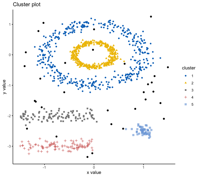
How many clusters do you see?

Why should we use DBSCAN?

Let’s see how K-Means deals with this dataset

Why should we use DBSCAN?

Now how about DBSCAN?

How does DBSCAN work?

Quick recap: \(\epsilon\)-neighbourhood

• Given a distance \(\epsilon\), the \(\epsilon\)-neighbourhood of a point is the number of points within distance at most \(\epsilon\) of it.

• In this example, \(\epsilon\)-neighbourhood of D is 6 if \(\epsilon\) is 2.

DSBSCAN takes two parameters:

• \(\epsilon\) or eps: does that sound familiar?

  That’s because it is! The parameter eps defines the radius of the neighborhood around a point x. This is what we called the \(\epsilon\)-neighborhood of x earlier

• minPts : it’s simply the minimum number of points within \(\epsilon\) radius

How does DBSCAN work?

A few definitions:

• Any point \(x\) in the data set, with a neighbour count greater than or equal to MinPts, is a core point
• \(x\) is a border point, if the number of its neighbors is less than MinPts, but it belongs to the \(\epsilon\)-neighborhood of some core point \(z\).
• If a point is neither a core nor a border point, then it is called a noise point or an outlier.

The figure shows the different types of points (core, border and outlier points) using MinPts = 6:

• \(x\) is a core point because \(neighbours_\epsilon(x)=6\)
• \(y\) is a border point because \(neighbours_\epsilon(y)<MinPts\), but it belongs to the \(\epsilon\)-neighborhood of the core point \(x\).
• Finally, \(z\) is a noise point.

A few more definitions:

• Direct density reachable: A point “A” is directly density reachable from another point “B” if: i) “A” is in the \(\epsilon\)-neighborhood of “B” and ii) “B” is a core point. E.g \(y\) is directly density reachable
• Density reachable: A point “A” is density reachable from “B” if there are a set of core points leading from “B” to “A.
• Density connected: Two points “A” and “B” are density connected if there are a core point “C”, such that both “A” and “B” are density reachable from “C”.

In density-based clustering, a cluster is defined as a group of density connected points.

How does DBSCAN work?

1. For each point \(x_i\), compute the distance between \(x_i\) and the other points. Find all neighbor points within distance eps of the starting point (\(x_i\)). Each point, with a neighbor count greater than or equal to MinPts, is marked as core point or visited.
2. For each core point, if it’s not already assigned to a cluster, create a new cluster. Find recursively all its density connected points and assign them to the same cluster as the core point.
3. Iterate through the remaining unvisited points in the data set.

The points that do not belong to any cluster are treated as outliers or noise.

If this explanation confuses you, you can have a look at this Youtube video

Plots source code

Important

Note that for most of the unsupervised learning techniques, no tidymodels functions are available. So, while we stay in the unsupervised learning realm, our code will follow base R conventions instead of the usual tidyverse/tidymodels ones.

# to run this code you might need to install packages `factoextra`, `fpc` and `dbscan`

library(factoextra) # library that contains the data set and allows us to visualise the clusters
library("fpc") # library that allows to use dbscan
library(dbscan)
library(ggplot2)

#loading the data
data("multishapes") 
df <- multishapes[, 1:2]
set.seed(123)

#plotting the data
ggplot(df, aes(x,y)) +
  geom_point()

Plots source code (continued)

# running k-means on the data
km.res <- kmeans(df, 5, nstart = 25)
#visualising the results of k-means
fviz_cluster(km.res, df,  geom = "point", 
             ellipse= FALSE, show.clust.cent = FALSE,
             palette = "jco", ggtheme = theme_classic())

#running DBSCAN
set.seed(123)
db <- fpc::dbscan(df, eps = 0.15, MinPts = 5)

# Plot DBSCAN results
fviz_cluster(db, data = df, stand = FALSE,
             ellipse = FALSE, show.clust.cent = FALSE,
             geom = "point",palette = "jco", ggtheme = theme_classic())

Anomaly detection

• Aim: detect abnormal patterns in the data
• Based on the notions of similarity/density we discussed previously, can you guess how this goal is accomplished?
• Clustering is one of the useful tools for this task: anomalies are points that are farthest from any other or points that lie in areas of low density

Anomaly detection through clustering

We already mentioned that DBSCAN detects outliers/anomalies.

If you want to find out more about what to when you get new data and about other clustering-based anomaly detection techniques, head this way.

Density-based anomaly detection : Local outlier factor (LOF)

• K-distance is the distance between a point and it’s K\(^{th}\) nearest neighbor.
• K-neighbors, denoted by \(N_k(A)\) is the set of points that lie in or on the circle of radius K-distance. K-neighbors can be greater or equal to the value of K.

Let’s see an example:

Let’s say we have four points: A, B, C, and D.

If K=2, K-neighbors of A include C, B and D and therefore \(||N_2(A)||\) = 3.

Density-based anomaly detection : Local outlier factor (LOF)

• Reachability distance:

  • Given two points \(x_j\) and \(x_i\), it is defined as the maximum of K-distance of \(x_j\) and the distance between \(x_i\) and \(x_j\). The distance measure is problem-specific (e.g Euclidean, Manhattan).
    
    

  Written more formally, this would look like this: \(RD(x_i,x_j)=\max(\textrm{K-distance}(x_j),\textrm{distance}(x_i,x_j))\)
  

  Said differently, if a point \(x_i\) belongs to the K-neighbors of \(x_j\) , the reachability distance will be K-distance of \(x_j\) (blue line), otherwise the reachability distance will be the distance between \(x_i\) and \(x_j\) (orange line)

Density-based anomaly detection : Local outlier factor (LOF)

• Local reachability density: It is inverse of the average reachability distance of a point A from its neighbors. The exact formula is:

  \(LRD_k(A)=\frac{1}{\sum_{x_j\in N_k(A)} \frac{RD(A,x_j)}{||N_k(A)||}}\)

  Intuitively according to the LRD formula, the higher the average reachability distance (i.e., neighbors are far from the point), the smaller the density of points are present around a particular point. This tells us how far a point is from the nearest cluster of points. Low LRD value imply that the closest cluster is far from the point.

  In other words, the LRD relies on the intuition that the longer the distance to the next neighbors, the sparser the area the respective point is located in. It tells us how far we have to travel from our point to reach the next point or cluster of points. So the lower it is, the less dense it is, the longer we have to travel.

Density-based anomaly detection: Local outlier factor (LOF)

• The LRD of each point is compared with the average LRD of its K-neighbors. We compute the local outlier factor or LOF which is the ratio of between the average LRD of the K-neighbors of point A and the LRD of A.
  

Or more specifically: \(LOF_k(A)=\frac{\sum_{x_j\in N_k(A)} LRD_k(x_j)}{||N_k(A)||}\times\frac{1}{LRD_k(A)}\)

• Intuitively, if the point is not an outlier (i.e is an inlier), the ratio of average LRD of neighbors is approximately equal to the LRD of the point (because the density of a point and its neighbors are roughly equal). In that case, LOF is nearly equal to 1. On the other hand, if the point is an outlier, the LRD of a point is less than the average LRD of neighbors. Then LOF value will be high.

• Generally, if LOF> 1, the point is considered an outlier, but that is not always true. Let’s say we know that we only have one outlier in the data, then we take the maximum LOF value among all the LOF values, and the point corresponding to the maximum LOF value will be considered as an outlier.

Density-based anomaly detection: Local outlier factor (LOF)

• 4 points: A(0,0), B(1,0), C(1,1) and D(0,3) and K=2.
• We will use LOF to detect one outlier (D) among these 4 points.
• First, calculate the K-distance, distance between each pair of points, and K-neighborhood of all the points with K=2

• We will be using the Manhattan distance as a measure of distance i.e \(d(x,y)=\sum_{i=1}^n |x_i-y_i|\)

Distance	Value
d(A,B)	1
d(A,C)	2
d(A,D)	3
d(B,C)	1
d(B,D)	4
d(C,D)	3

K-distance(A): since C is the 2\(^{nd}\) nearest neighbor of A, K-distance(A)=d(A,C) =2 K-distance(B): since A, C are the 2\(^{nd}\) nearest neighbor of B, K-distance(B)=distance(B,C) OR K-distance(B)=distance(B,A) = 1 K-distance(C): since A is the 2\(^{nd}\) nearest neighbor of C –> K-distance(C)=distance(C,A) =2 K-distance(D): since A,C are the 2\(^{nd}\) nearest neighbor of D –> K-distance(D)=distance(D,A) or K-distance(D)=distance(D,C) =3

• K-neighborhood (A) = {B,C} , \(||N_2(A)|| =2\)
  K-neighborhood (B) = {A,C}, \(||N_2(B)|| =2\)
  K-neighborhood (C)= {B,A}, \(||N_2(C)|| =2\)
  K-neighborhood (D) = {A,C}, \(||N_2(D)|| =2\)

Density-based anomaly detection: Local outlier factor (LOF)

We use the K-distance and K-neighbourhood to compute the LRD for each point

\(LRD_2(A)=\frac{1}{\frac{RD(A,B)+RD(A,C)}{||N_2(A)||}}=\frac{\frac{1}{1+2}}{2}=0.667\) \(LRD_2(B)=\frac{1}{\frac{RD(B,A)+RD(B,C)}{||N_2(B)||}}=\frac{\frac{1}{2+2}}{2}=0.50\) \(LRD_2(C)=\frac{1}{\frac{RD(C,A)+RD(C,B)}{||N_2(C)||}}=\frac{\frac{1}{1+2}}{2}=0.667\) \(LRD_2(D)=\frac{1}{\frac{RD(D,A)+RD(D,C)}{||N_2(D)||}}=\frac{\frac{1}{3+3}}{2}=0.337\)

\(LOF_2(A)=\frac{LRD_2(B)+LRD_2(C)}{||N_2(A)||}\times\frac{1}{LRD_2(A)}=\frac{0.5+0.667}{2}\times\frac{1}{0.667}=0.87\) \(LOF_2(B)=\frac{LRD_2(A)+LRD_2(C)}{||N_2(B)||}\times\frac{1}{LRD_2(B)}=\frac{0.667+0.667}{2}\times\frac{1}{0.5}=1.334\) \(LOF_2(C)=\frac{LRD_2(A)+LRD_2(B)}{||N_2(C)||}\times\frac{1}{LRD_2(C)}=\frac{0.667+0.5}{2}\times\frac{1}{0.667}=0.87\) \(LOF_2(D)=\frac{LRD_2(A)+LRD_2(C)}{||N_2(D)||}\times\frac{1}{LRD_2(D)}=\frac{0.667+0.667}{2}\times\frac{1}{0.337}=2\)

The highest LOF among the four points is LOF(D). Therefore, D is an outlier/anomaly.

Density-based anomaly detection: Local outlier factor (LOF)

Pros

• LOF identifies outliers based on the local neighborhood
• A point will be considered as an anomaly/outlier if it is at a short distance from an extremely dense cluster.
• A global approach may not consider that point as an outlier. But LOF can effectively identify local outliers. It gives better results than the global approach to find outliers

Cons

• Since LOF is a ratio, it is difficult to interpret
• There is no threshold value to LOF and the selection of a point as an anomaly/outlier is user-dependent (and also problem-dependent)

See (Breunig et al. 2000) for more details on LOF.

For a detailed demo (with code and PCA!) on (simulated) fraud dataset, head over this way.

Another popular method of anomaly detection is called isolation forest: if you’d like to learn about it, see (Liu, Ting, and Zhou 2008)

Dimensionality reduction

Principal component analysis

What is Principal Component Analysis (PCA)?

Principal component analysis (PCA) is a technique that transforms high-dimensions data into lower-dimensions while retaining as much information as possible.

What does “information” mean in the PCA context?

variance!

Let’s take a look at the variance formula: \(S^2=\frac{\sum (x_i-\bar{x})}{n-1}\) (i.e the average degree to which each point differs from the mean \(\bar{x}\)). Nowhere in the formula is there an association with information. So where does it come from.

Principal component analysis

Say we’re playing a guessing game and are trying to guess the height of three people.

Person	Height (cm)
Alex	145
Ben	160
Chris	185

If looking at the silhouettes below

Then, we can guess Chris is A, B is Alex and C is Ben

Principal component analysis

If we now try to figure who hides behind these silhouettes

when we have this new group of people

Person	Height (cm)
Tabby	171
Jon	172
Alex	173

this suddenly becomes tougher!
That’s because in the earlier group, the height varied substantially. In the same way, when our data has a higher variance, it holds more information. Variance is information

Principal component analysis

Now suppose we also have the people’s weights to try and differentiate them. Is it useful at all?

Person	Height (cm)	Weight(kg)
Alex	145	68
Ben	160	67
Chris	185	70

• Not exactly, we still rely on height only
• Intuitively, we have just reduced our data from 2-dimensions to 1-dimension. The idea is that we can selectively keep the variables with higher variances and then forget about the variables with lower variance.

Principal component analysis

What if height and weight had the same variance?

In that case, PCA combines height and weight linearly to create two new (uncorrelated/orthogonal) variables that capture the total variance of both height and weight: these are the principal components.

• In general, with real data, you don’t get a principal component that captures 100% of the variances.

• Performing a PCA will give us N number of principal components, where N is equal to the dimensionality of our original data (i.e the number of features in the data).

• From this list of principal components, you usually choose the least number of principal components that would explain the most amount (i.e the most variance) of our original data.

If you want additional explanations on PCA, check out this Youtube video or this link or this link (more theoretical).

What’s next?

• Text mining and topic modelling

References

Arthur, David, and Sergei Vassilvitskii. 2007. “K-Means++ the Advantages of Careful Seeding.” In Proceedings of the Eighteenth Annual ACM-SIAM Symposium on Discrete Algorithms, 1027–35. SODA. New Orleans Louisiana: Society for Industrial; Applied Mathematics3600 University City Science Center Philadelphia, PAUnited States. https://dl.acm.org/doi/10.5555/1283383.1283494.

Breunig, Markus M., Hans-Peter Kriegel, Raymond T. Ng, and Jörg Sander. 2000. “LOF: Identifying Density-Based Local Outliers.” In Proceedings of the 2000 ACM SIGMOD International Conference on Management of Data, 93–104. Dallas Texas USA: ACM. https://doi.org/10.1145/342009.335388.

Liu, Fei Tony, Kai Ming Ting, and Zhi-Hua Zhou. 2008. “Isolation Forest.” In 2008 Eighth IEEE International Conference on Data Mining, 413–22. Pisa, Italy: IEEE. https://doi.org/10.1109/ICDM.2008.17.