🗓️ Week 08
Machine Learning II
DS101 – Fundamentals of Data Science
17 Nov 2025
Different models draw different boundaries

Many possible separating lines
If the two classes can be separated, there isn’t just one solution: there are infinitely many valid separating lines.
SVM asks:
Among all separating lines that classify the training data correctly, which one is the safest?

The maximum-margin idea
SVM chooses the line that maximises the margin — the safest separation between classes.
- Margin = the distance between the decision boundary and the nearest training points from each class
- These nearest points (one or more per class) are the support vectors
- These critical points alone determine the SVM boundary
- The SVM chooses the line that keeps these points as far away as possible
- A wider margin usually leads to better generalisation

Soft margins: real data is messy
Perfect separation is rare:
- Spotify hits vs flops
Soft margins: real data is messy
- Benign vs malignant tumours
- Many social-science datasets
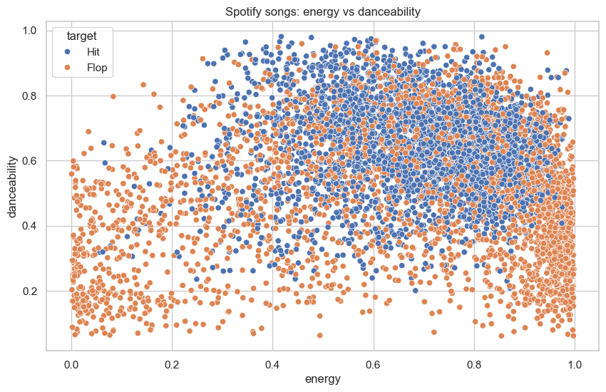
Soft-margin SVM on Spotify hits/flops
Hit vs flop songs using energy and danceability:
- The two classes overlap heavily
- No straight line can separate them well
- Soft-margin SVM finds a compromise boundary balancing width vs classification errors
This plot also shows why linear SVM is a poor choice for this dataset.

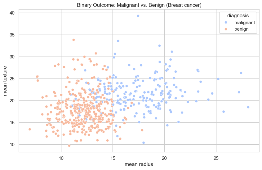
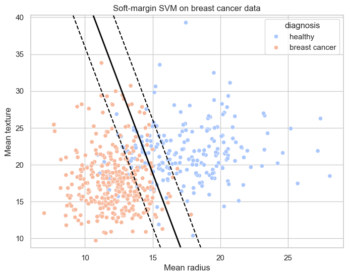
Soft-margin SVM on breast cancer data
Benign vs malignant tumours (2D projection):
- Noticeable overlap between classes
- Soft-margin SVM avoids forcing any brittle perfect separator
- The balance between errors vs margin width is visible in the geometry
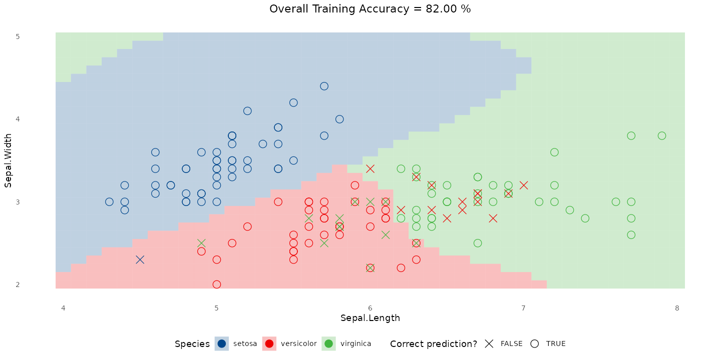
Kernel SVM on iris (three species)
RBF kernel finds smooth, curved regions separating all three iris species:
Non-linear SVM on Spotify songs
For Spotify hits/flops, a curved RBF boundary works far better than any straight line:

🎧 SVM on Spotify Songs
Performance Metrics:
Classification Report:
              precision    recall  f1-score   support

        Flop       0.89      0.73      0.80       960
         Hit       0.77      0.91      0.83       960

    accuracy                           0.82      1920
   macro avg       0.83      0.82      0.82      1920
weighted avg       0.83      0.82      0.82      1920
Confusion Matrix:

📊 Interpretation:
- Accuracy improved slightly to ~82 %.
- The SVM correctly classifies more hits than the tree or logistic regression.
- It handles curved, overlapping relationships better than straight-line or boxy splits.
- But SVMs are harder to interpret — we lose the clear “if–then” logic of trees.
💡 Conceptual takeaway: The model isn’t just smarter — it’s smoother. It balances flexibility and generalization without memorizing the data.
Model comparison

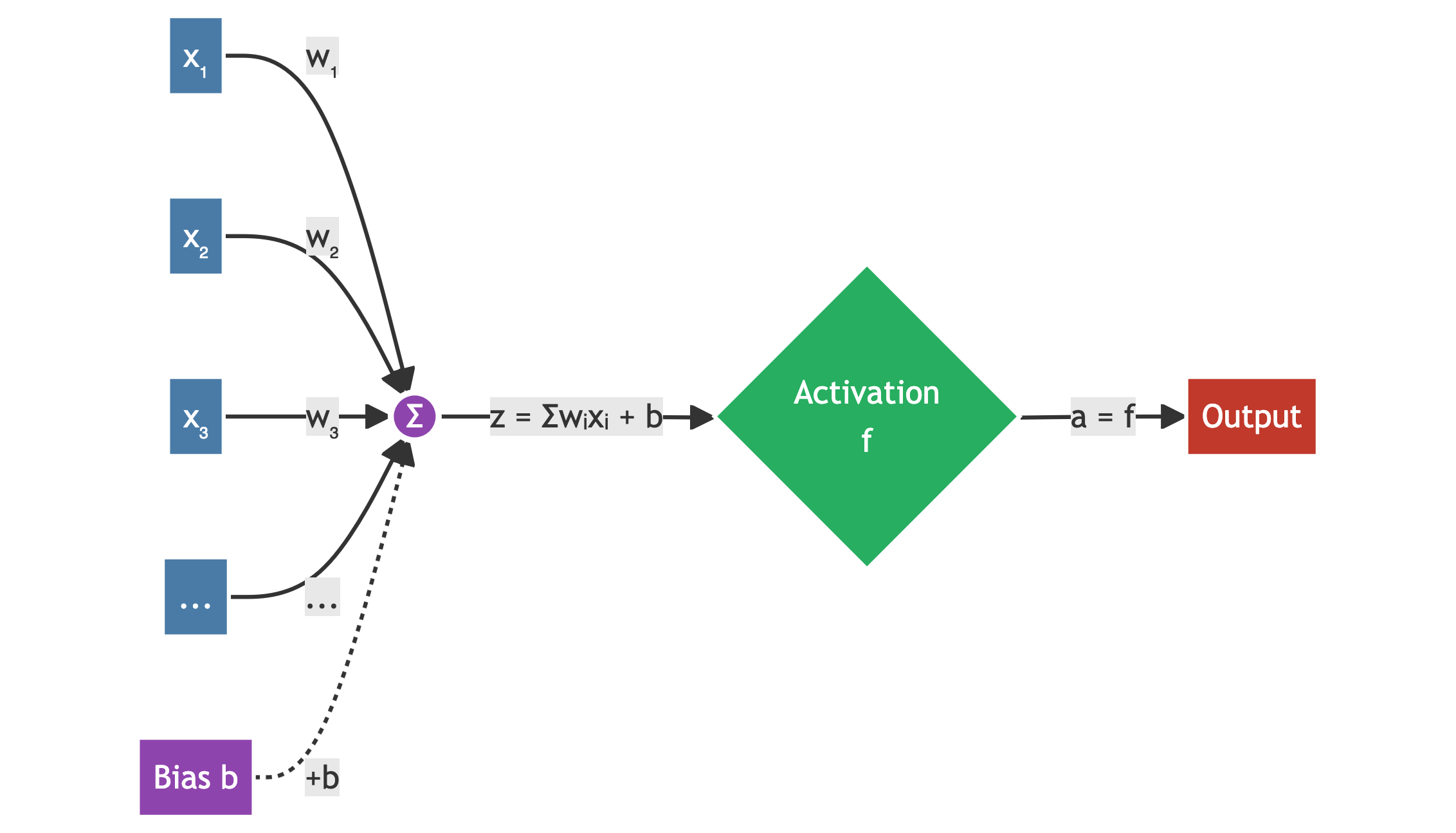
The neuron: weighted input → transformation
A neuron computes:
\[ z = w_1 x_1 + w_2 x_2 + \dots + w_n x_n + b \]
\[ \text{output} = f(z) \]
Where:
- \(w_i\): weights
- \(b\): bias
- \(f(\cdot)\): activation function (e.g., ReLU, sigmoid)
It’s a small, flexible function that can bend a decision boundary.
Diagram:

Stacking neurons: learning in layers
By linking neurons into layers, networks can learn richer patterns:
- Layer 1 → basic combinations of inputs
- Layer 2 → combinations of Layer 1 features
- Layer 3 → higher-level structure
Each layer transforms what the previous one learned.
What is deep learning?
Deep learning uses networks with multiple successive layers. A deep network:
- Applies several weighted transformations in sequence
- Learns features at different levels of abstraction
- Can represent highly non-linear relationships
Formally:
\[ x \rightarrow f_1(x) \rightarrow f_2(f_1(x)) \rightarrow \dots \rightarrow f_L(\dots) \]
Diagram:
Why deep learning works
Deep networks build hierarchical representations:
Audio:
- Lower layers: simple frequency patterns
- Mid layers: rhythm / timbre
- Higher layers: genre or mood
Images:
- Edges → shapes → objects
Tabular data:
- Interactions between features
- Automatically learned combinations
- Flexible, non-linear boundaries
Depth = expressive power.
But deep networks process sequences poorly on their own, which leads to…
![]()
Attention: learning what to focus on
Attention solves the context problem by letting each word:
Look directly at any other word and decide how important it is.
It assigns attention weights that highlight relevant parts of the input.
This enables:
- Long-range understanding
- Better handling of references and ambiguity
- Efficient learning on long sequences
Diagram:

Transformers: architecture built around attention
Transformers remove recurrence and rely entirely on attention:
- Inputs receive positional encodings (to reflect word order)
- Each word can use information from any other word
- Layers of multi-head attention + feed-forward networks refine meaning
- Fully parallel operations → fast training
- Highly scalable → extremely deep and large models
Transformers now power:
- GPT-style language models
- Machine translation
- Image generation (e.g., DALL·E)
- Speech and audio processing
- Protein folding (AlphaFold)
- Most modern AI systems
Canonical architecture diagram: ![]()
A first look at the data
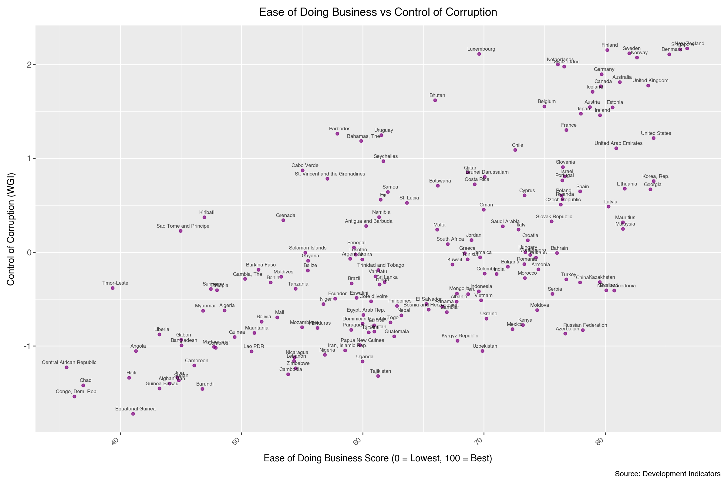
Even without labels, you might notice:
- some countries that sit close together
- others that are clearly far apart
- a kind of band or gradient
- a few isolated points that don’t fit the main pattern
At this stage, these are just visual impressions, not conclusions.
We will analyse this dataset properly later in a live clustering demo.
Distance metrics: continuous data
Euclidean distance
The most familiar one:
\[ d(A,B) = \sqrt{\sum_{i=1}^n (A_i - B_i)^2} \]
- straight-line (“as the crow flies”) distance
- sensitive to large differences in any coordinate

Use when:
- features are continuous
- on similar scales (after normalisation if needed)
- you care about overall geometric distance
Examples:
- country indicators (GDP, life expectancy)
- song features (energy, tempo)
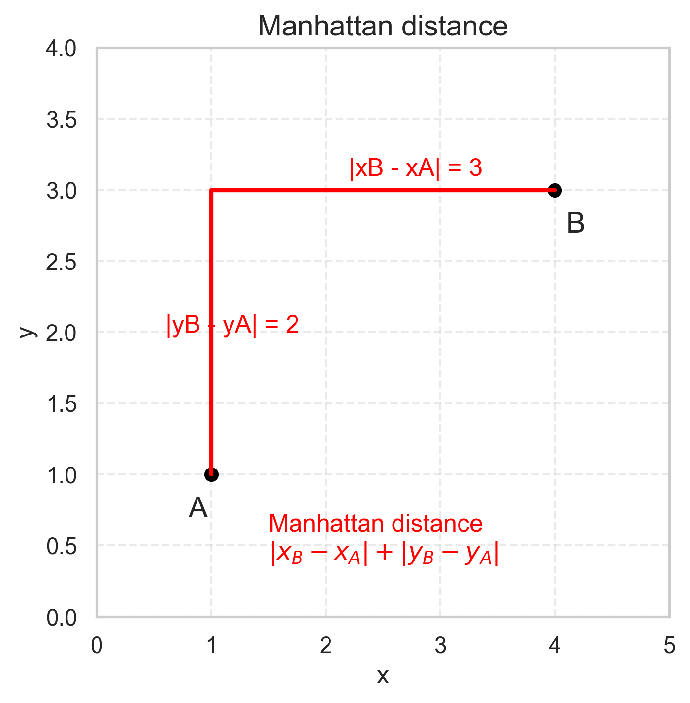
Manhattan distance
Also called L1 distance:
\[ d(A,B) = \sum_{i=1}^n |A_i - B_i| \]
- like walking in a grid (“city block” distance)
- less sensitive to single big differences
Use when:
- you care about additive differences
- robustness to outliers is important
- features change in discrete steps
Example:
- survey responses encoded as 1–5 (Likert-type), after appropriate preprocessing
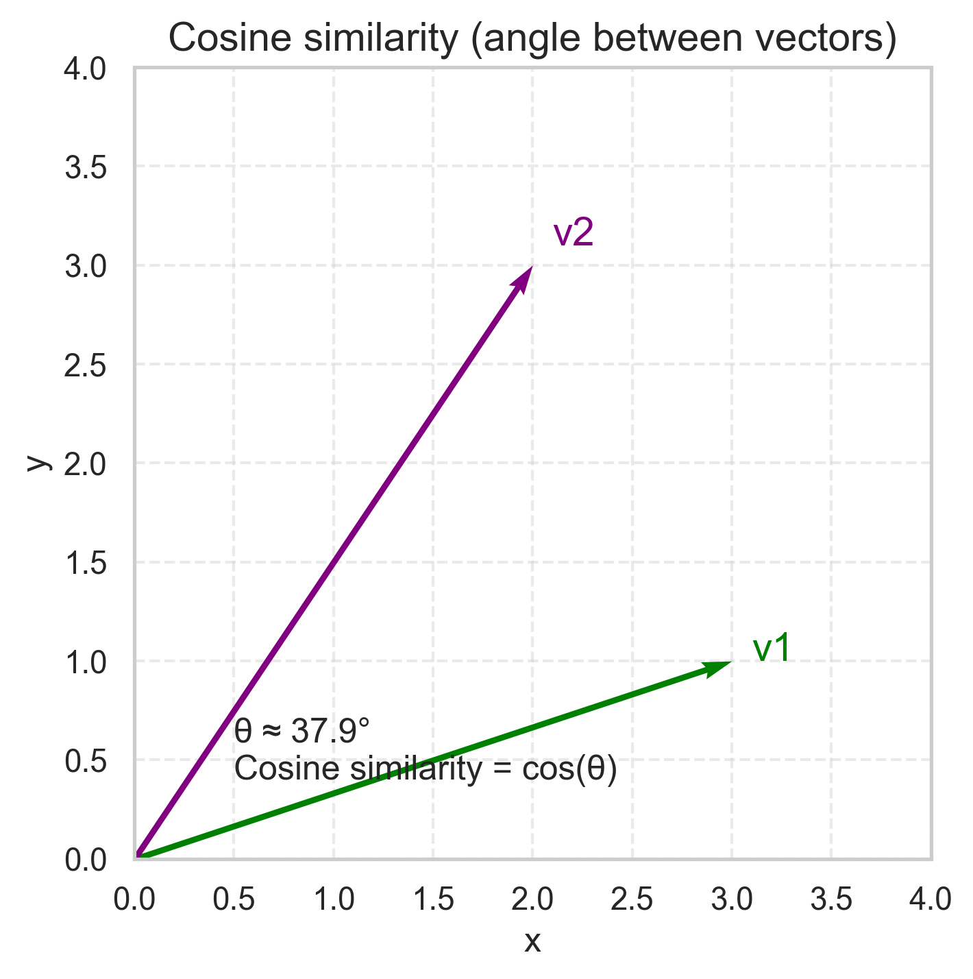
Cosine similarity
Instead of distance, a similarity:
\[ S_C(A,B) = \frac{\sum_i A_i B_i} {\sqrt{\sum_i A_i^2} \sqrt{\sum_i B_i^2}} \]
- measures the angle between two vectors
- ignores overall magnitude (length)
Useful when:
- direction matters more than scale
- you care about proportions, not absolute values
Examples:
- text (word-frequency vectors)
- budget allocations (% of spending in each category)
- survey profiles where we care about pattern, not absolute intensity
Visualising ε-neighbourhoods
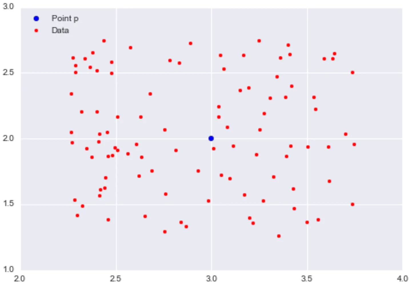
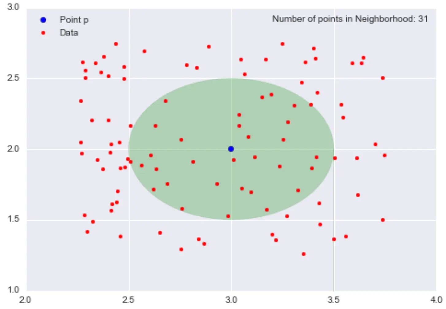
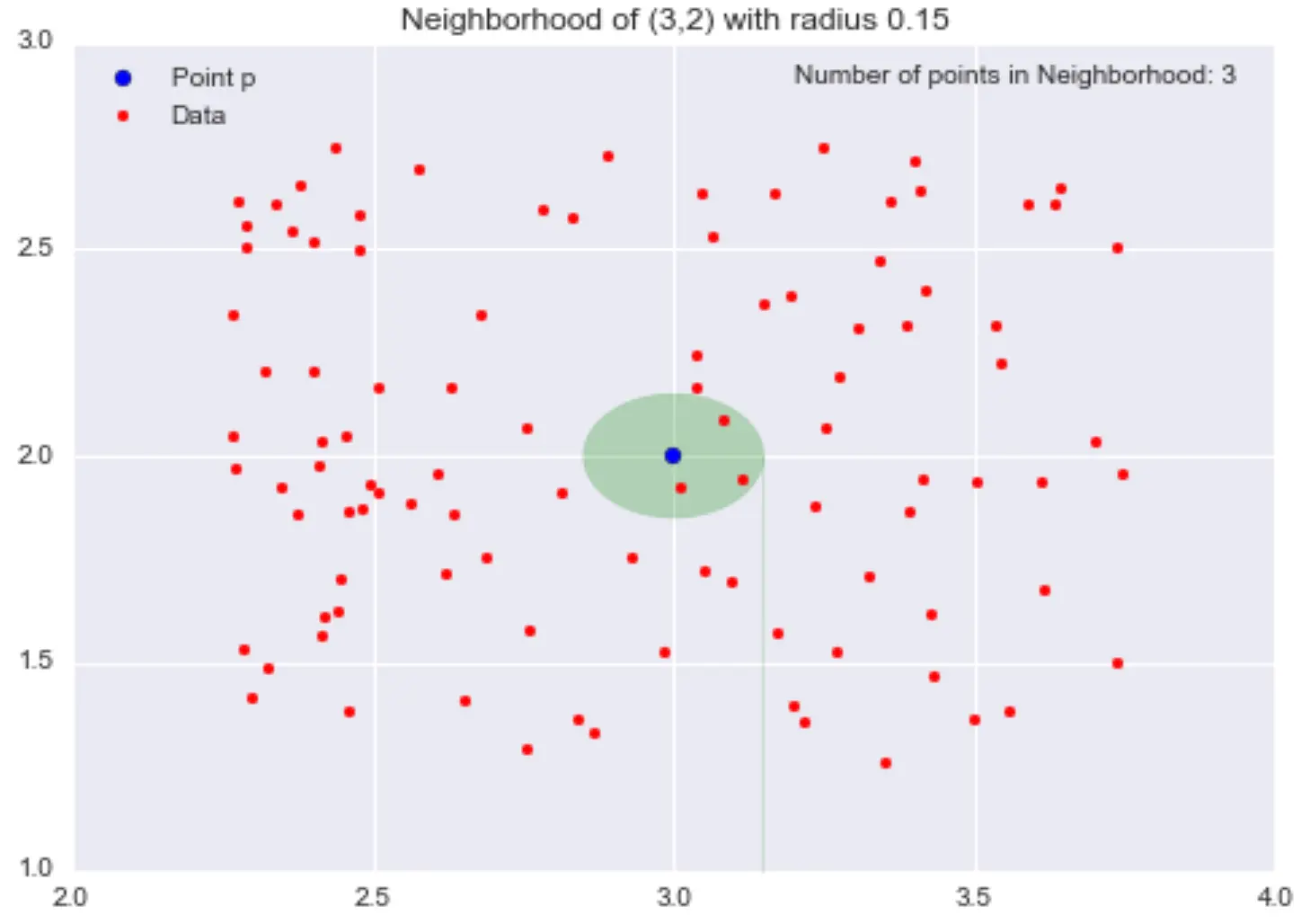
- With larger ε, each point has more neighbours
- With smaller ε, each point has fewer neighbours
We can think of:
density = number of points / volume (or area)
K-means: visual walkthrough
A live demo: see here
Step 1: choose K

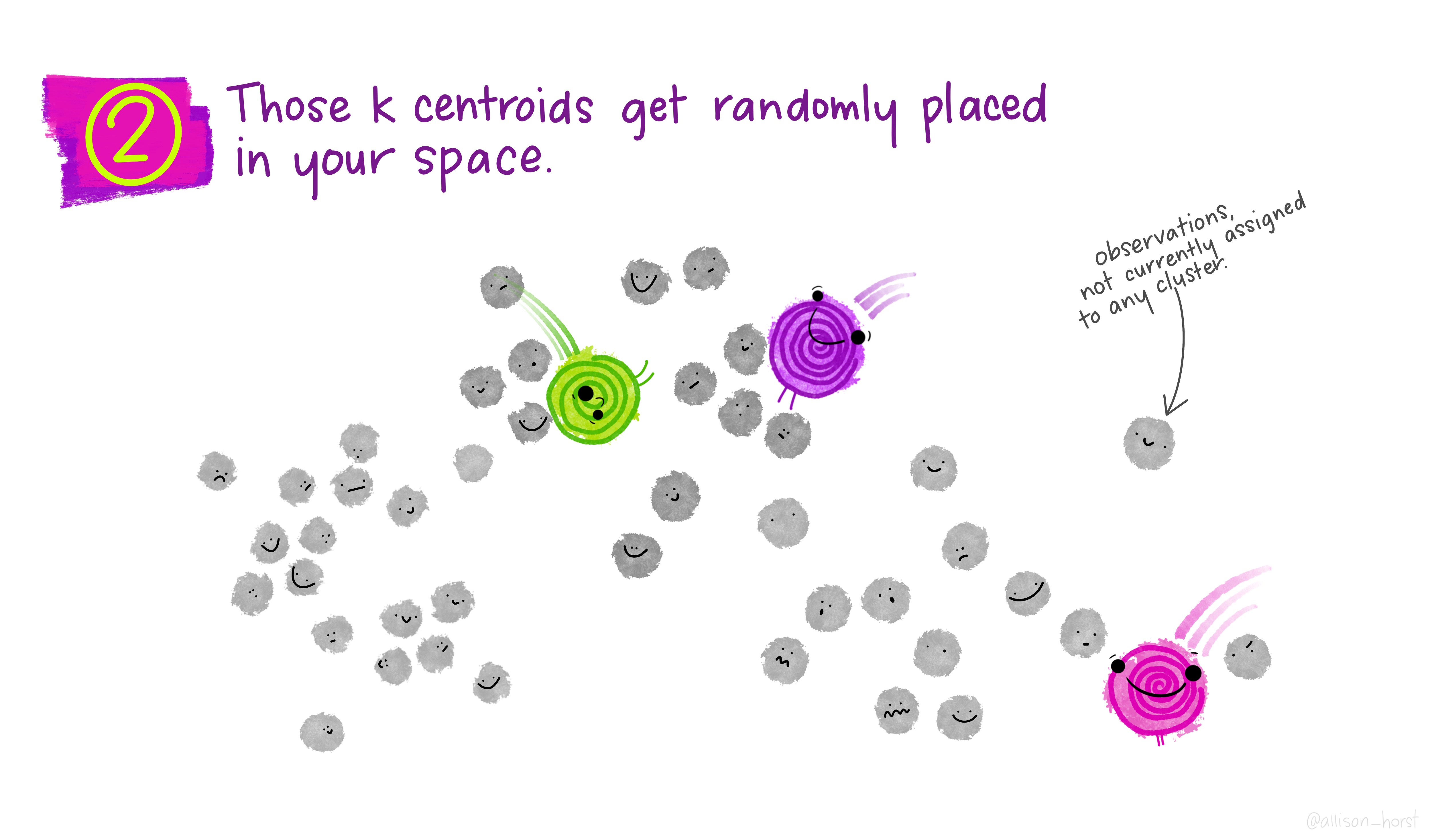
Step 2: initialise centroids

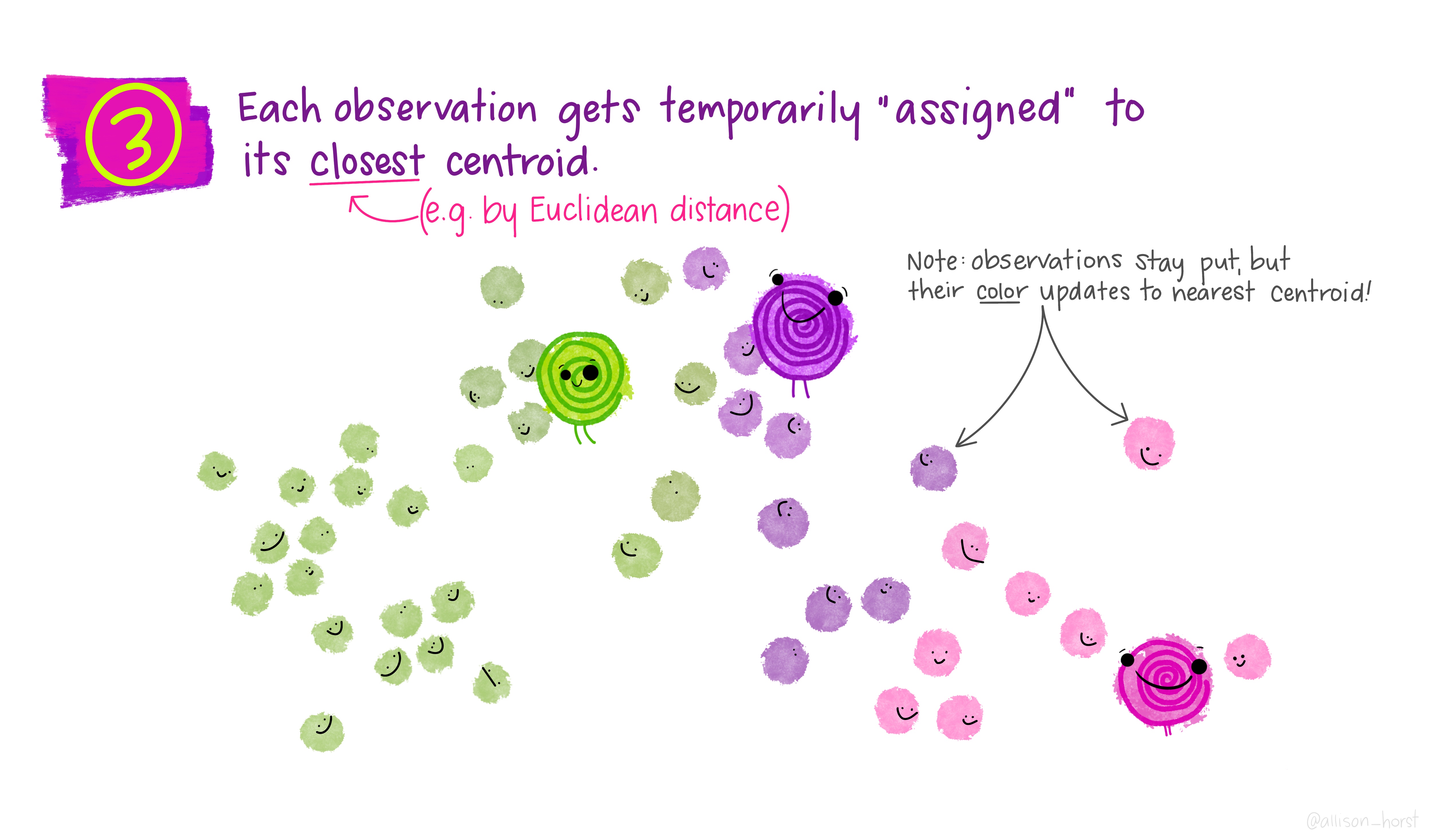
Step 3: assign to nearest centroid
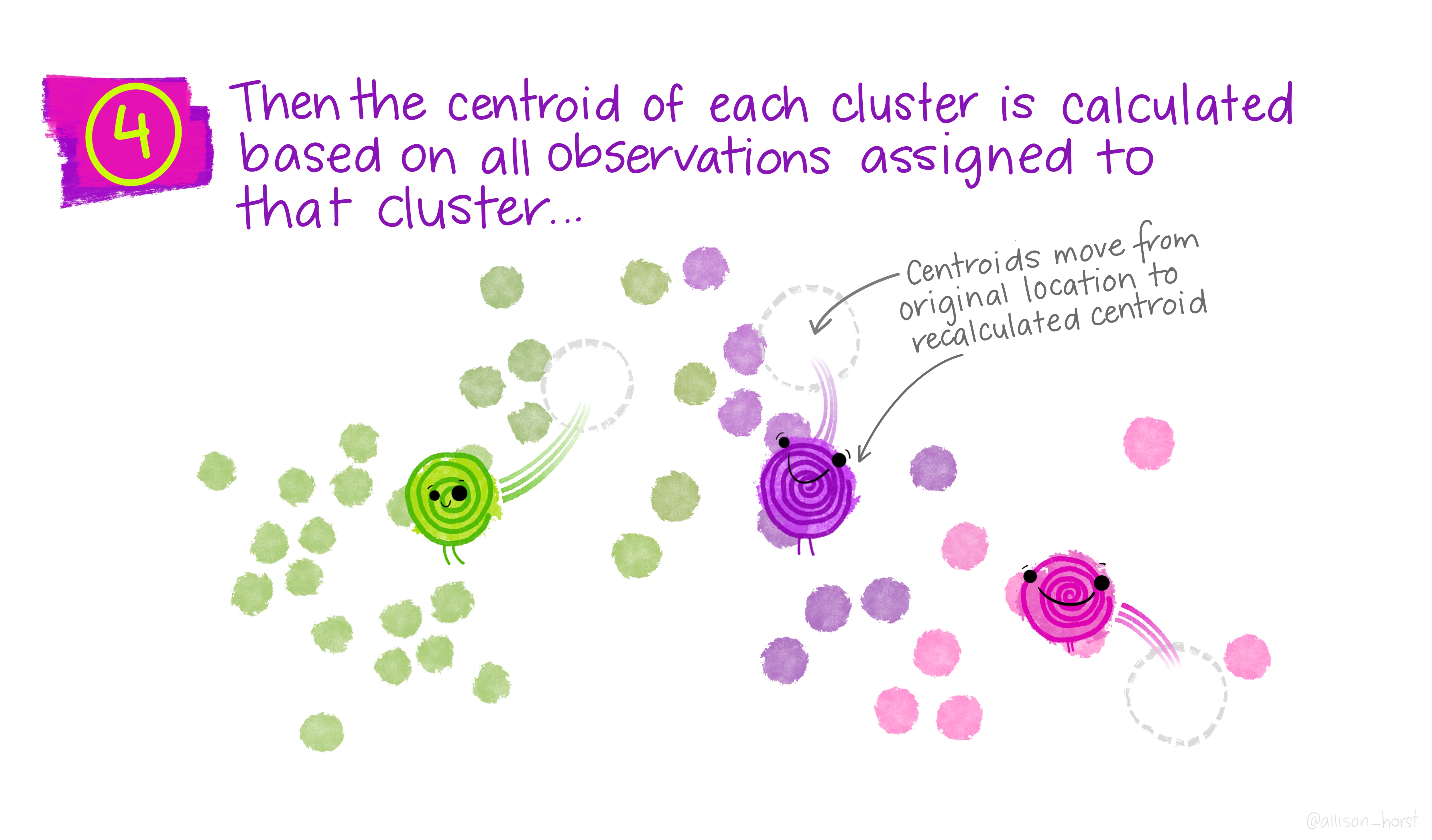
Step 4: recompute centroids
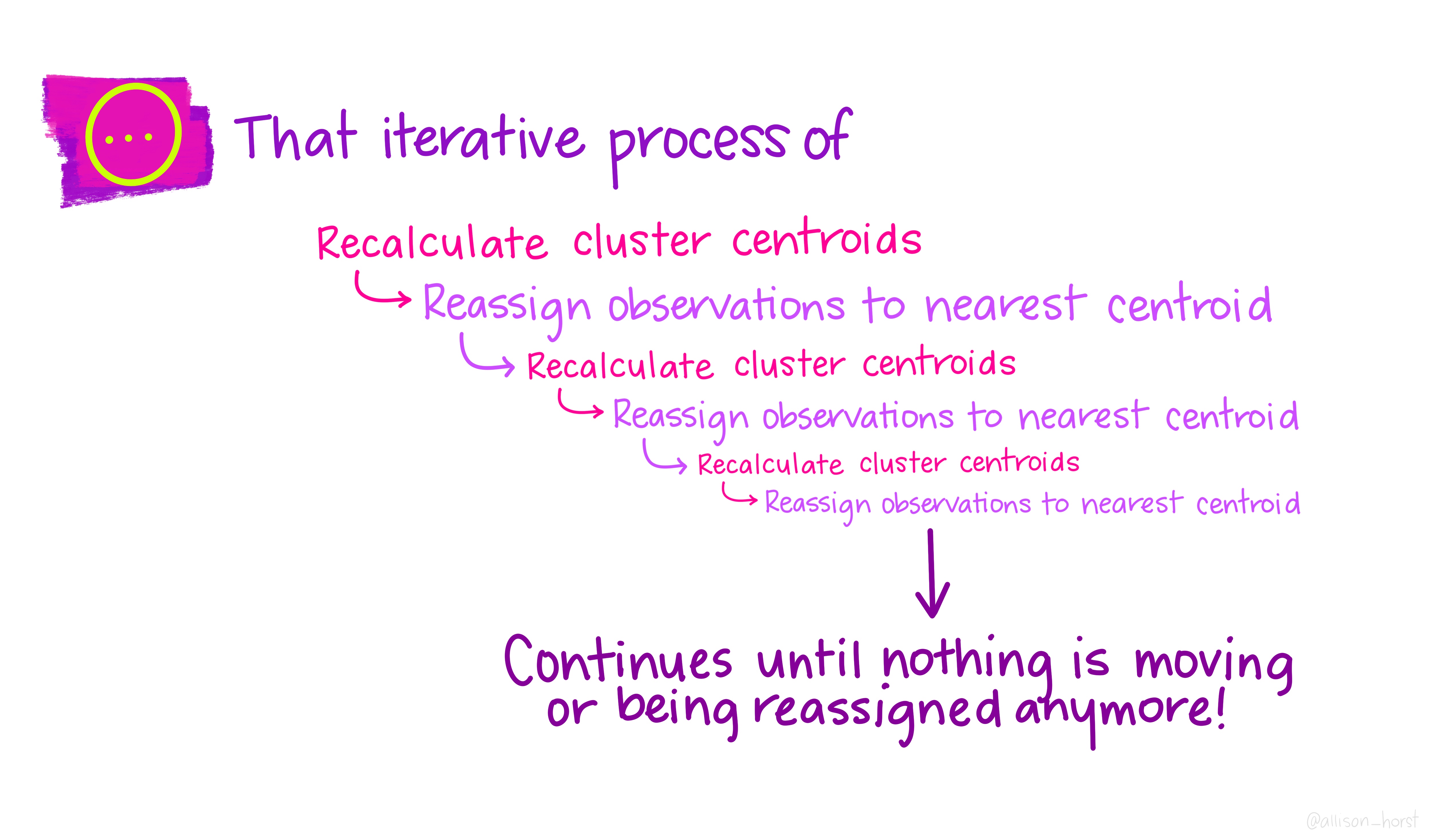
K-means: iteration

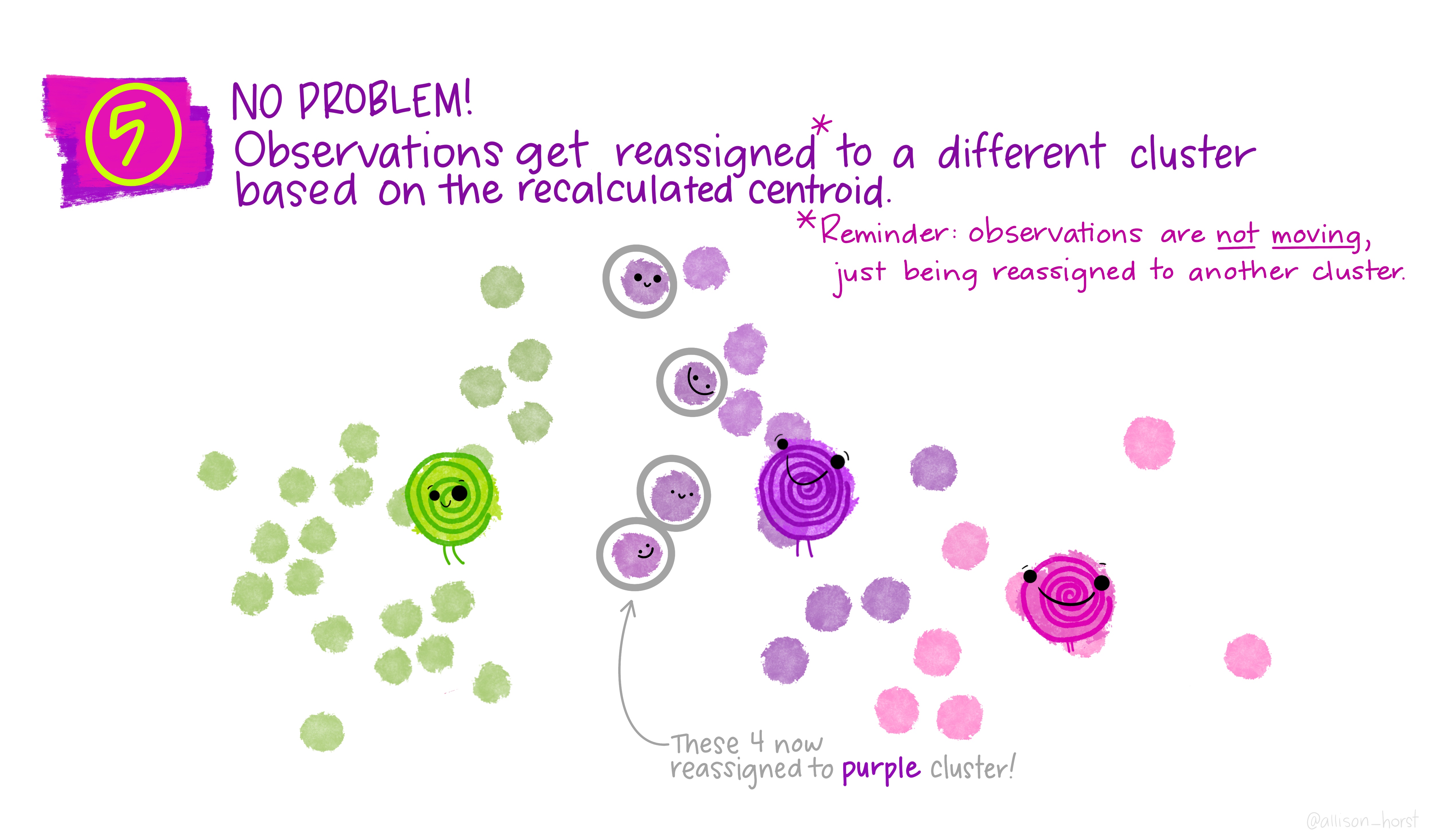

Assignments change, then centres update, then assignments change, etc.
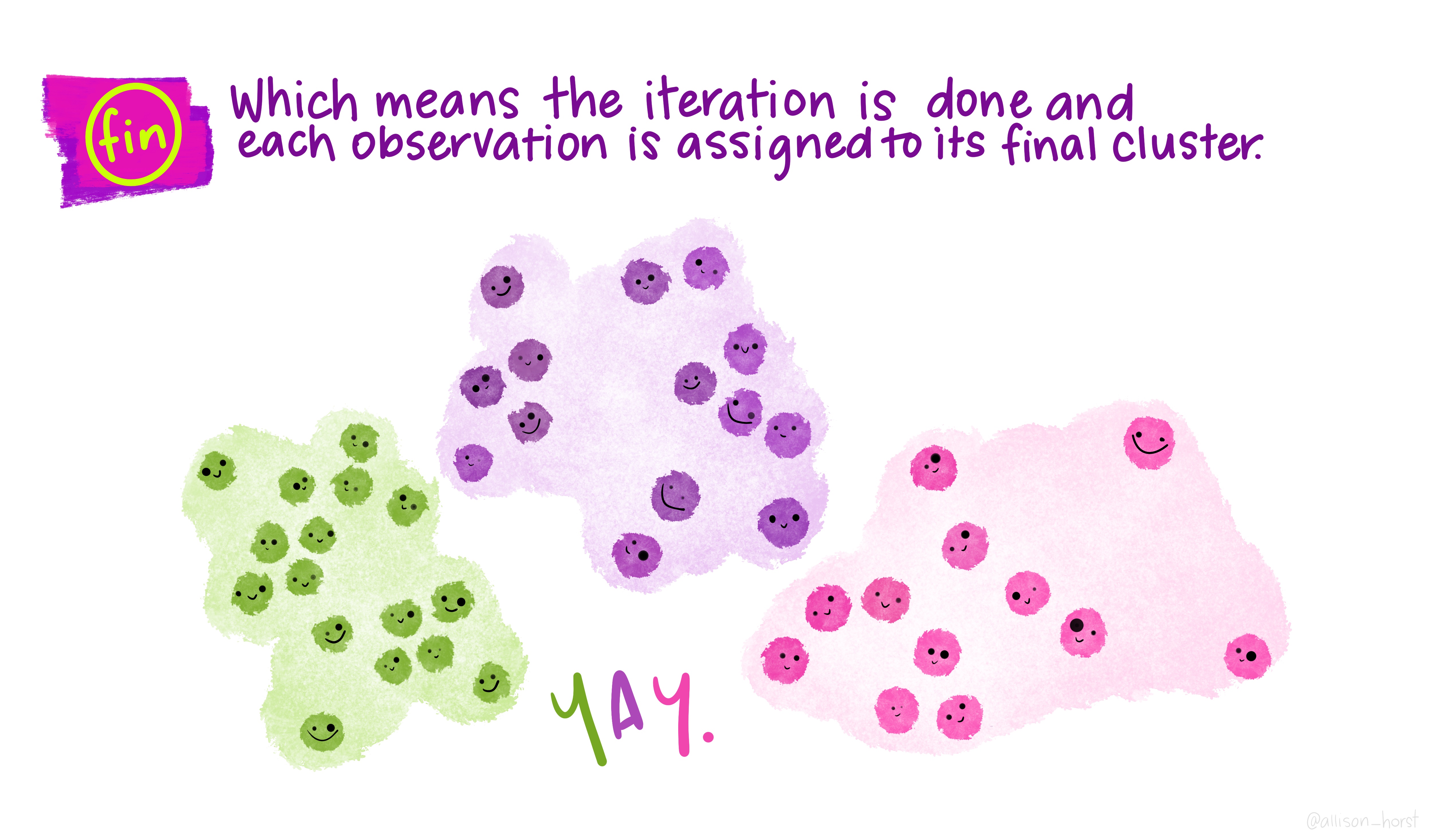
K-means: convergence


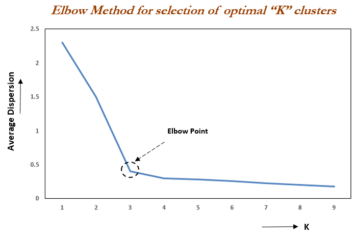
Choosing K: the elbow method
One popular heuristic:
- Run K-means for different values of \(K\) (e.g., 1 to 10).
- For each K, compute WCSS.
- Plot WCSS vs K.
- Look for an “elbow”: a point where the curve bends and extra clusters give diminishing returns.