🗓️ Week 09
Unstructured data: basics of text mining
DS101 – Fundamentals of Data Science
25 Nov 2024
⏪ Unsupervised learning: A brief recap
- We discovered what unsupervised learning was about:
- the algorithms do not rely on labeled data to learn
- the focus is on learning hidden patterns in the data without human intervention (and without labels!)
- There are various types of unsupervised learning that have wide applications:
- clustering
- association rule mining
- dimensionality reduction
- anomaly detection
Similarity
- Notion central to clustering and anomaly detection
- Quantifies how data samples are related or close to each other
- Often expressed as a number between 0 and 1
- The higher it is, the closer the points are together, i.e “the more similar” they are
- Based on a distance function
Similarity
Examples of common distance/similarity functions:
Real-valued data:
Euclidian distance: \(d(A,B)=\sqrt{\sum_{i=1}^n |A_i-B_i|^2}\)
Cosine distance: \(S_C(A,B)=\frac{\sum_{i=1}^n A_iB_i}{\sqrt{\sum_{i=1}^n A_i^2}\sqrt{\sum_{i=1}^n B_i^2}}\)
where A and B are two n-dimensional vectors of attributes, and \(A_i\) and \(B_i\) the \(i\)th components of vectors A and B respectively
String similarity:
- Hamming distance: given two strings of equal length, it is the number of positions at which the corresponding symbols (i.e either letters, bits, or decimal digits) are different e.g:
- 0000 and 1111 is 4
- cat and car is 1
- call and cold is 2
Similarity
Examples of common distance/similarity functions:
String similarity
Levenstein distance: given two strings, it’s the minimal number of edits (substutions, deletions, insertions) needed to turn one string into another e.g:
The Levenshtein distance between kitten and sitting is 3, since the following 3 edits change one into the other, and there is no way to do it with fewer than 3 edits:
- kitten → sitten (substitution of “s” for “k”),
- sitten → sittin (substitution of “i” for “e”),
- sittin → sitting (insertion of “g” at the end).
Set similarity:
A set is a collection of items with no order or repetition. Sets are typically used to represent relationships or associations between objects or even people.
- Jaccard index: it is often used in recommendation systems and social media analysis and measures the similarity between two sets based on the number of items present in both sets relative to the total number of items
\(J(A,B)=\frac{|A\cap B|}{|A\cup B|}\)
where A and B are two sets, \(|A\cap B|\) the number of items included in both sets and \(|A\cup B|\) the total number of items
Density
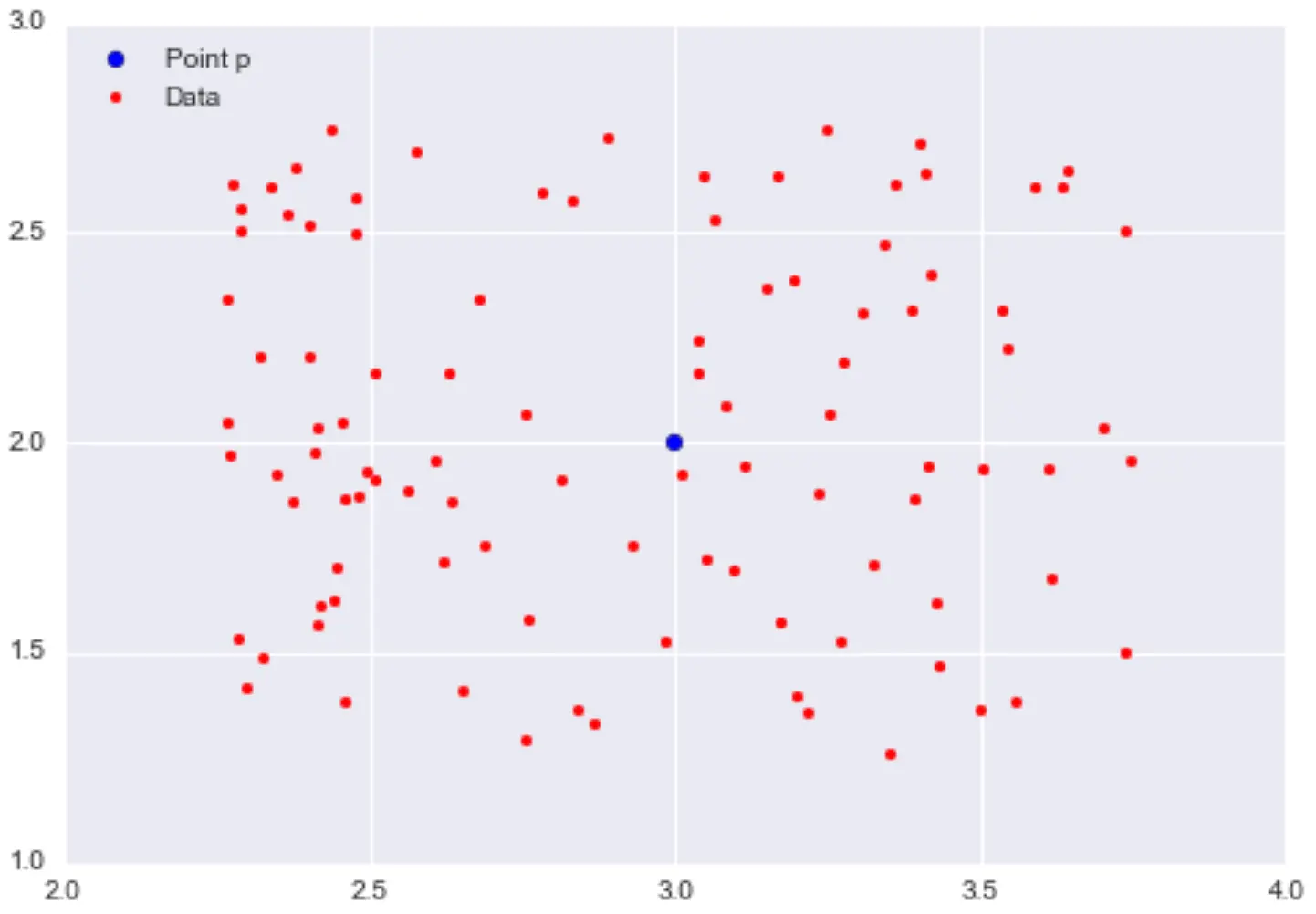
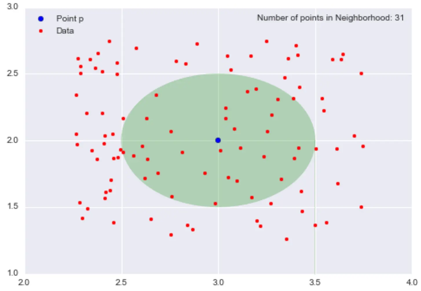
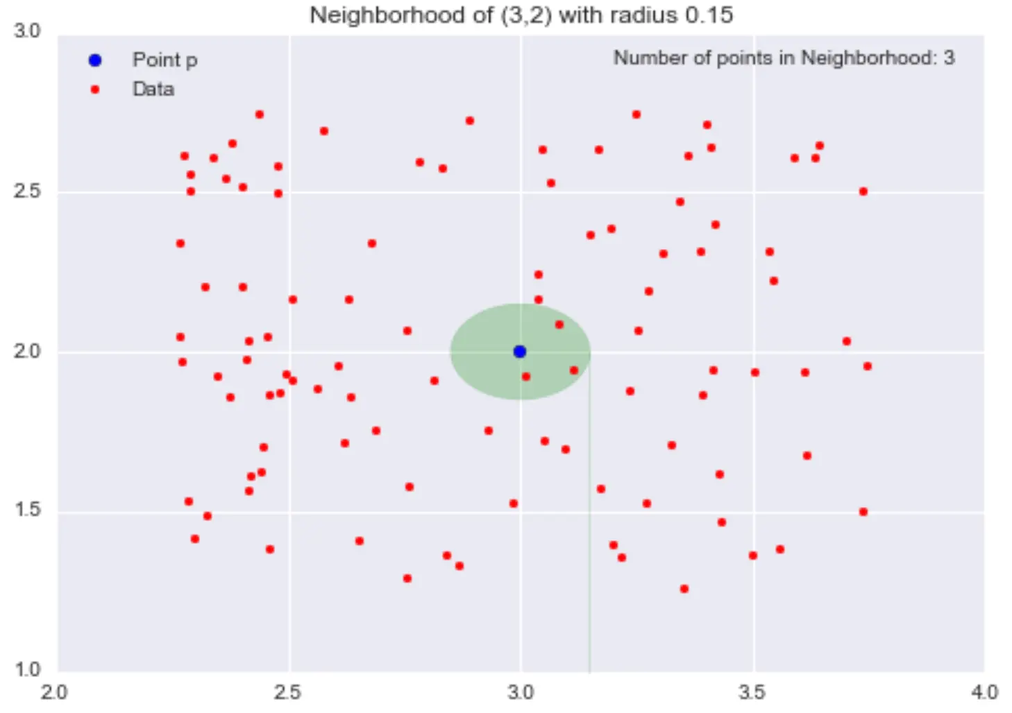
\(\epsilon\)-neighbourhoods:
- given \(\epsilon>0\) and a point \(p\), the \(\epsilon\)-neighbourhood of \(p\) is the set of points that are at distance at most \(\epsilon\) away from \(p\)
Example:
(Images source: https://domino.ai/blog/topology-and-density-based-clustering)
Density (continued)
Density:
- Roughly defined, \(\textrm{density}=\frac{\textrm{"mass"}}{\textrm{"volume"}}\)
- If we go back to our previous example, the “mass” would be the number of points in an \(\epsilon\)-neighbourhood centered in \(p\) and the “volume” the area of radius \(\epsilon\) centered around \(p\)
Example:

If we take the figure above, the local density estimation at \(p=(3,2)\) is \(\frac{31}{0.25\pi} \approx 39.5\)
- Number that is meaningless on its own
- If we calculate the densities of all points in our dataset, we could say that points within the same neighbourhood and similar local densities belong to the same cluster \(\rightarrow\) General principle of density-based clustering methods e.g DBSCAN (see (Ester et al. 1996) for more details on the DBSCAN algorithm)
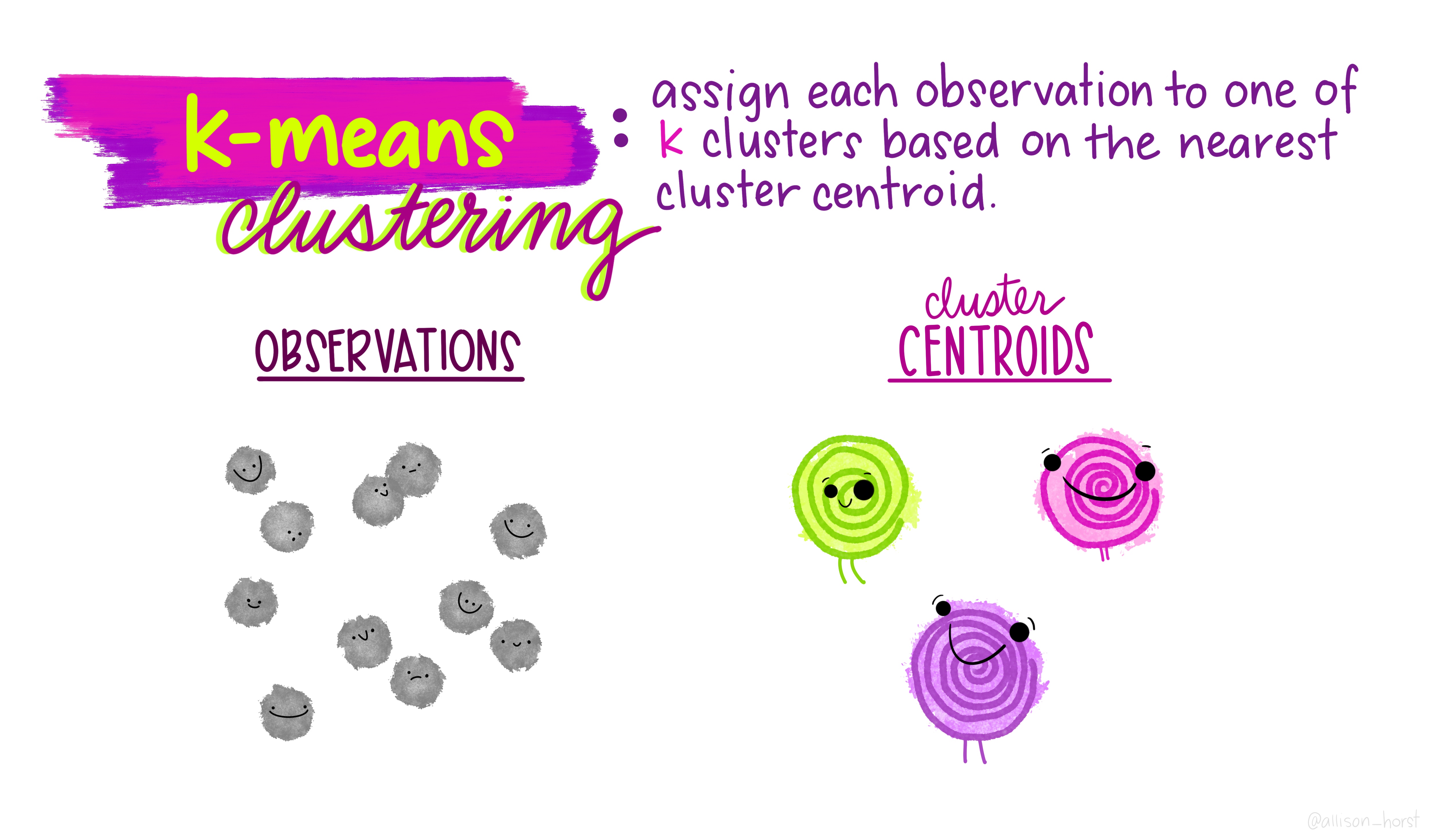
An example of clustering algorithm: k-means
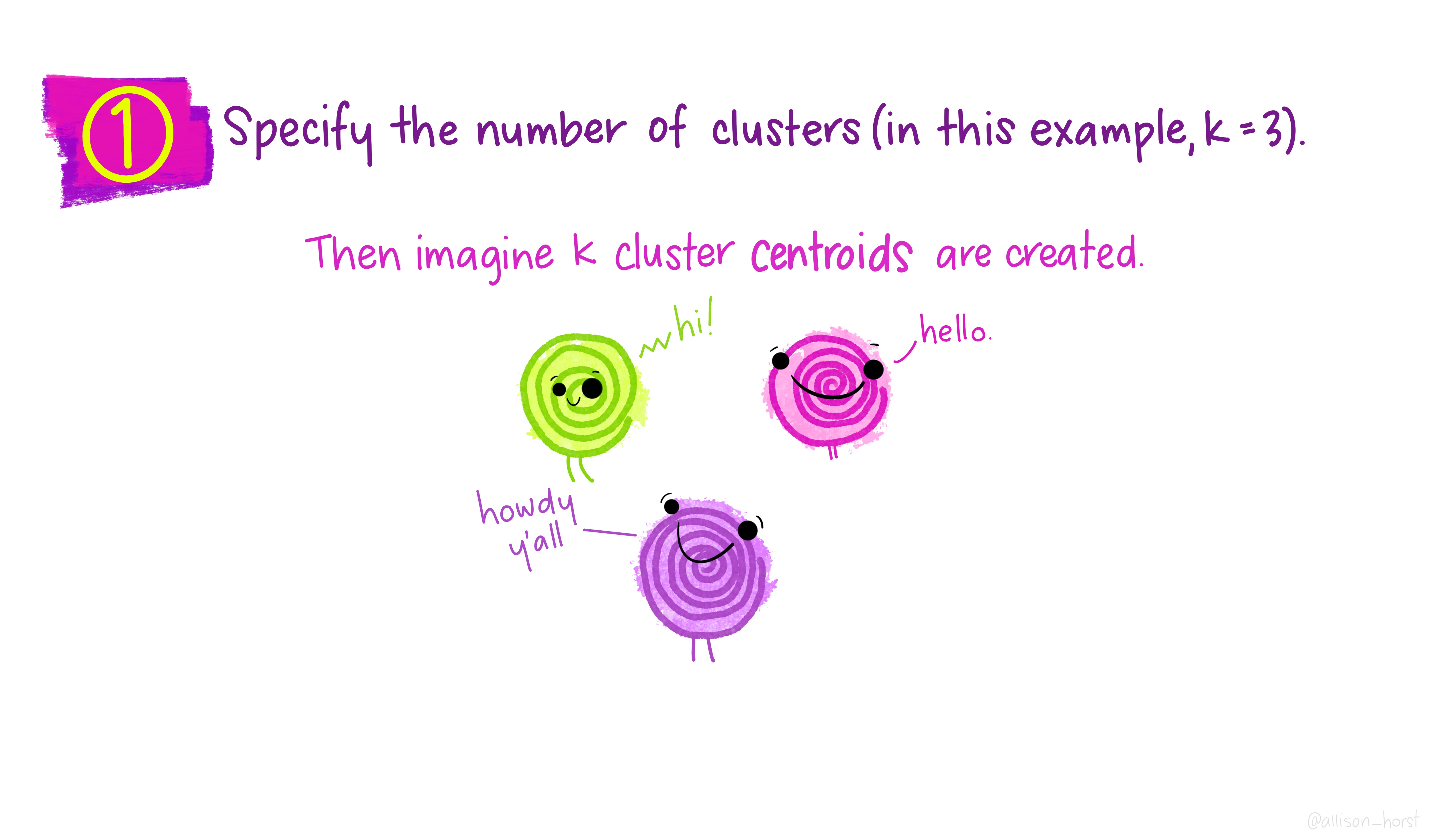
An example of clustering algorithm: k-means (continued)
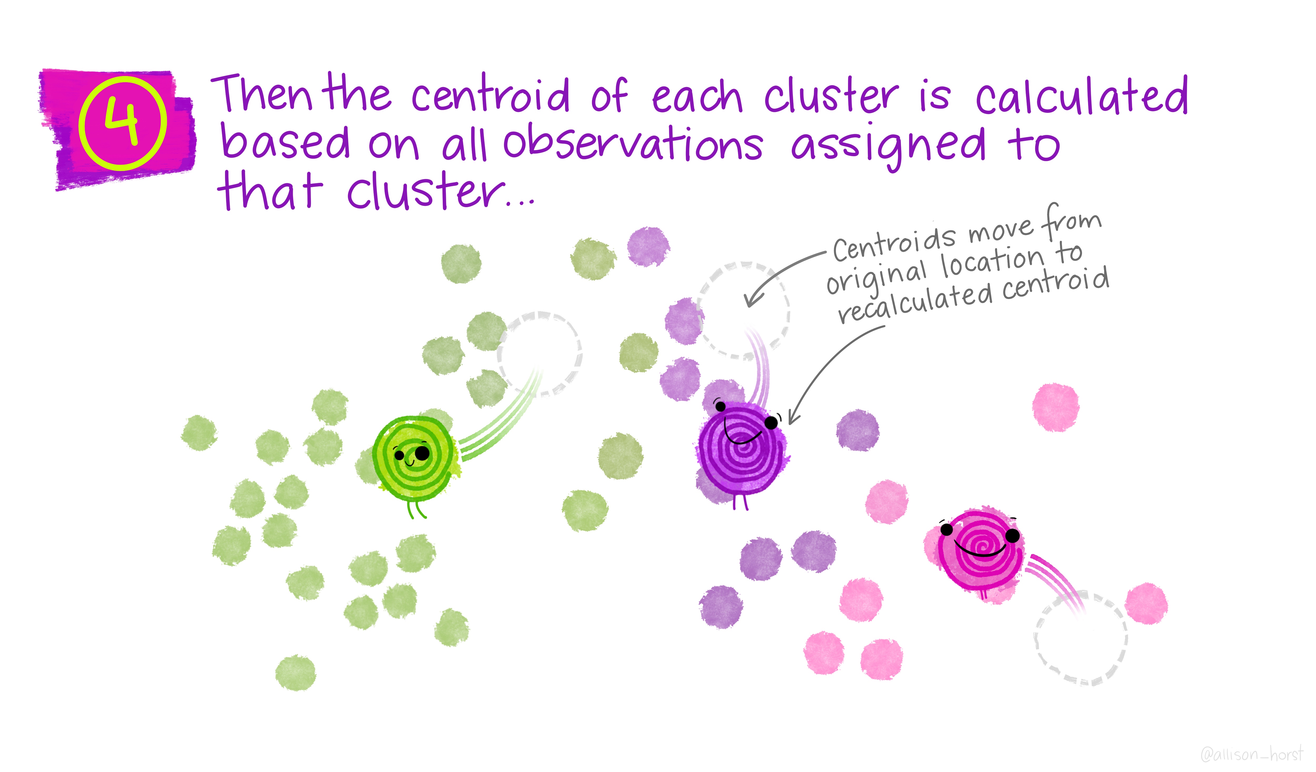
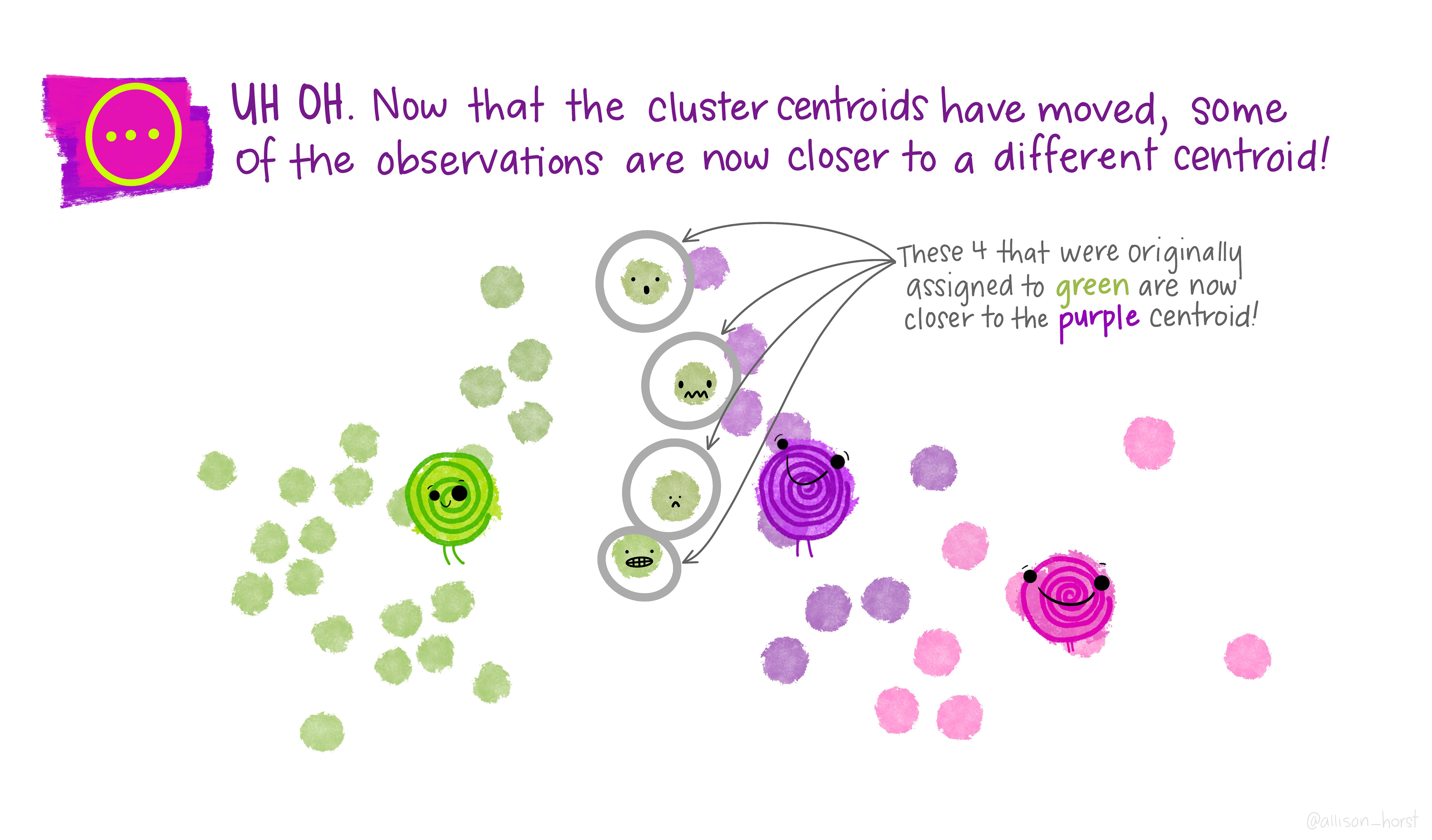
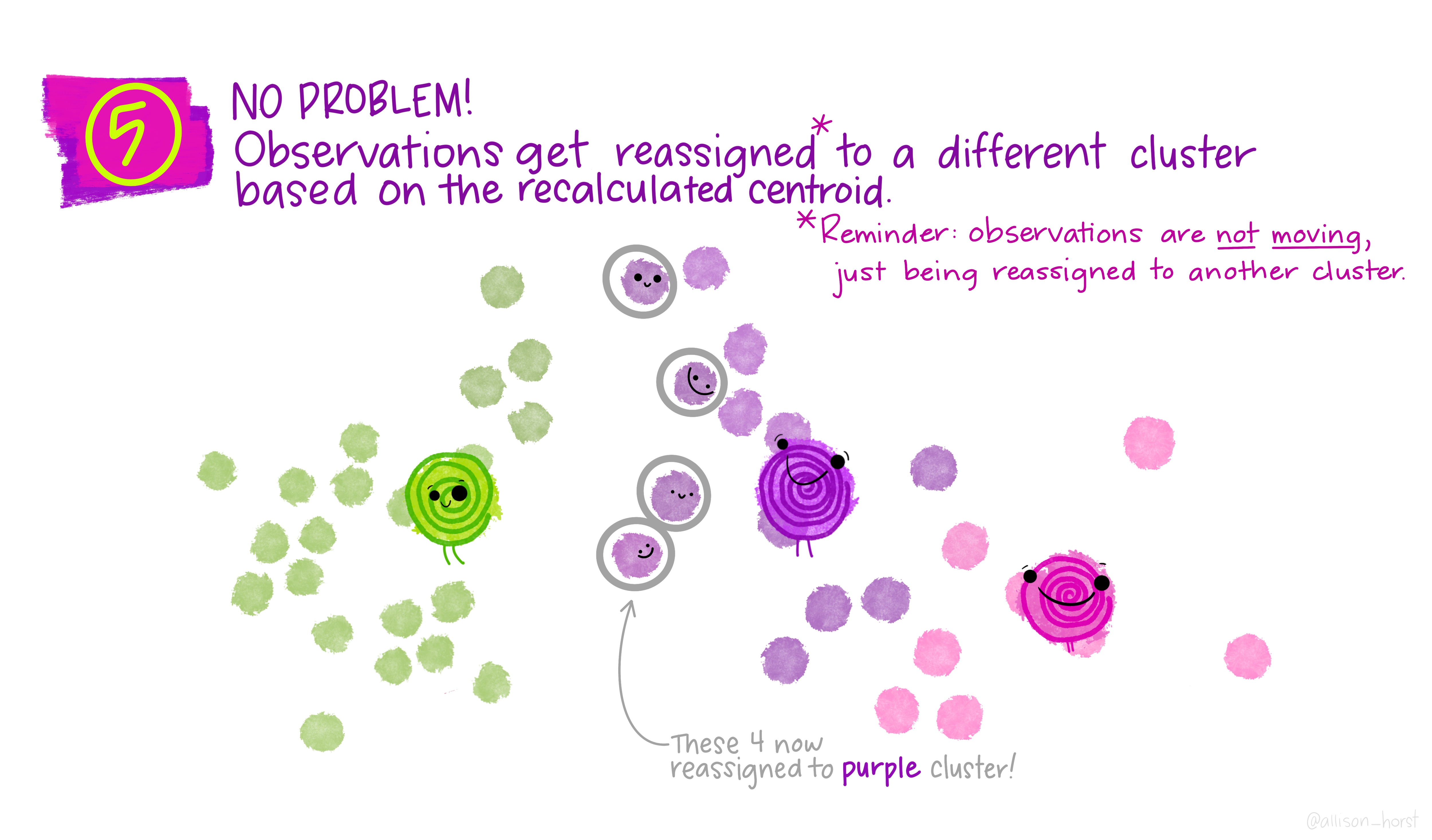
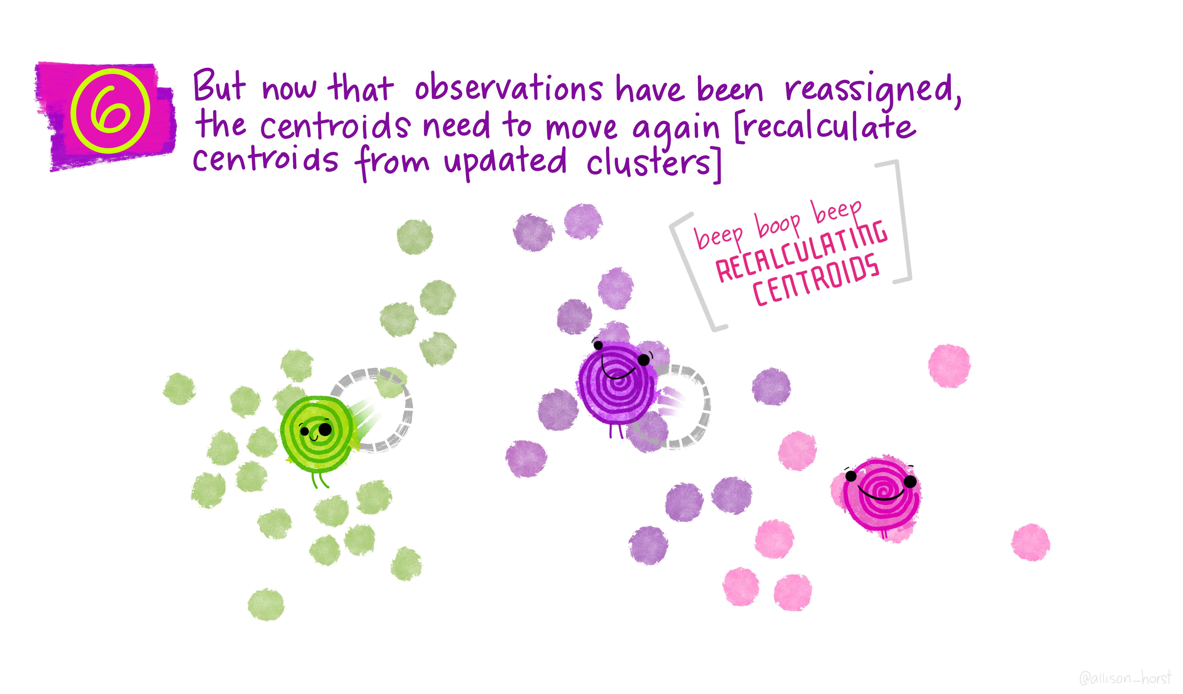
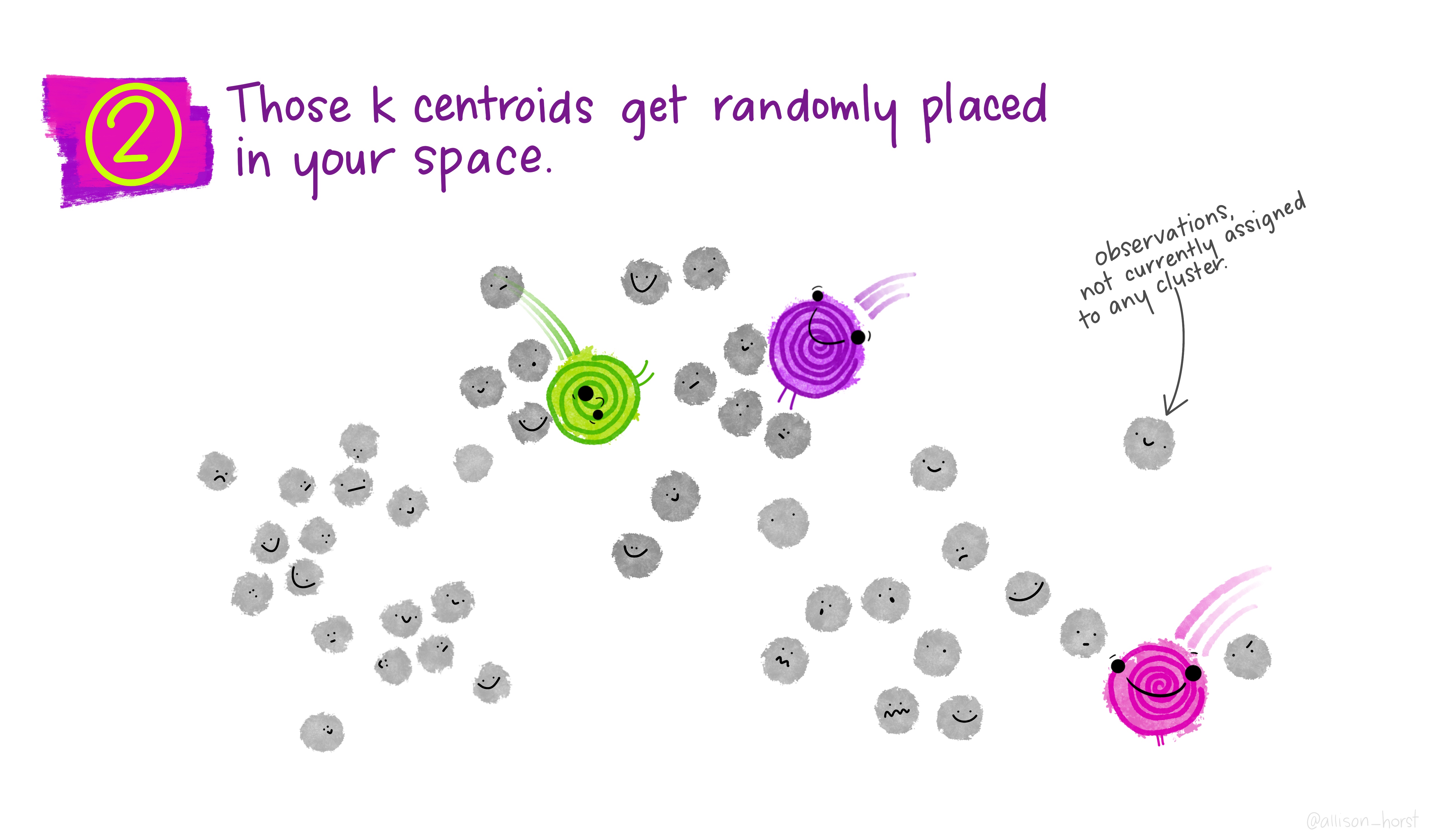
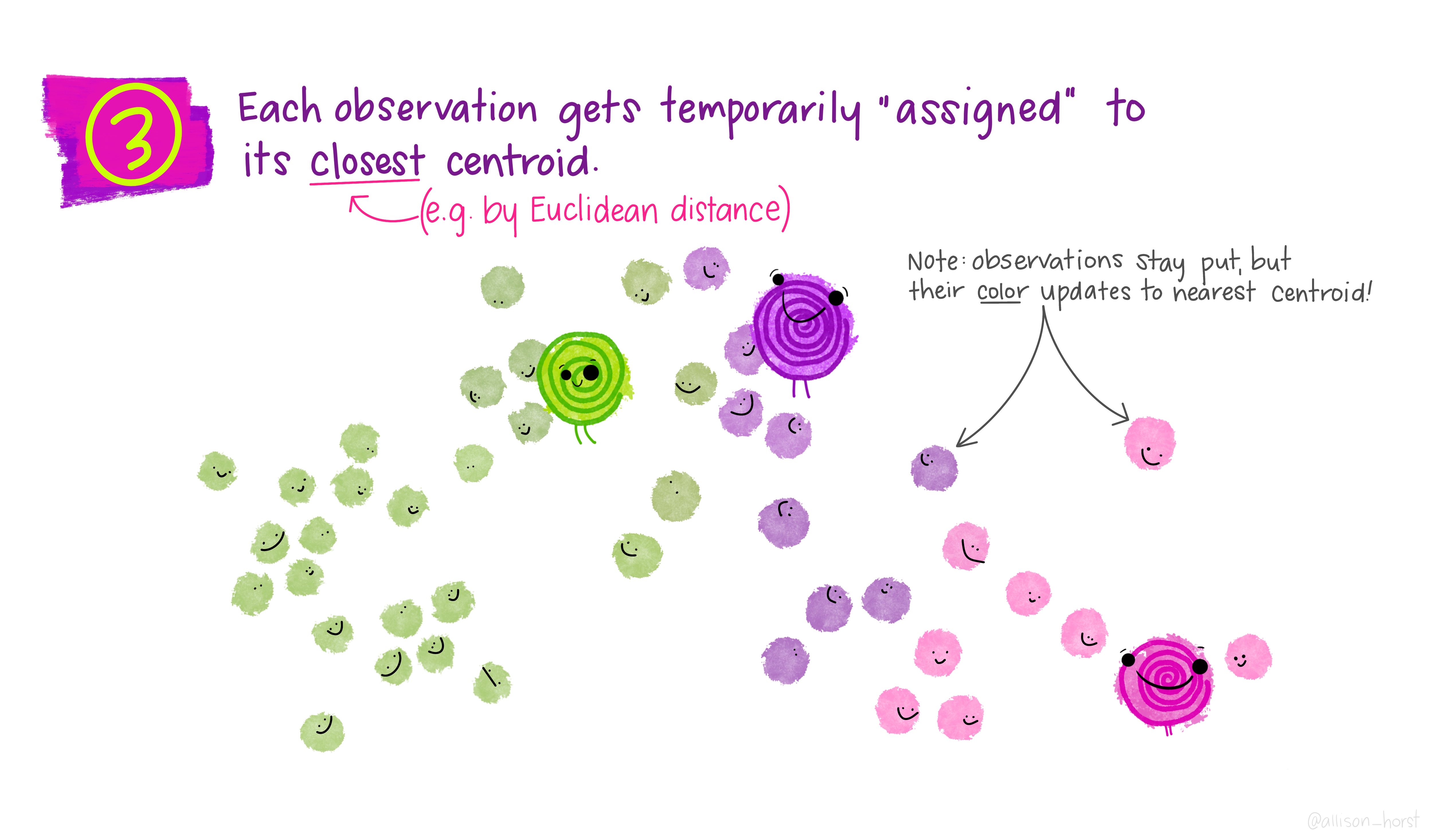
An example of clustering algorithm: k-means (continued)
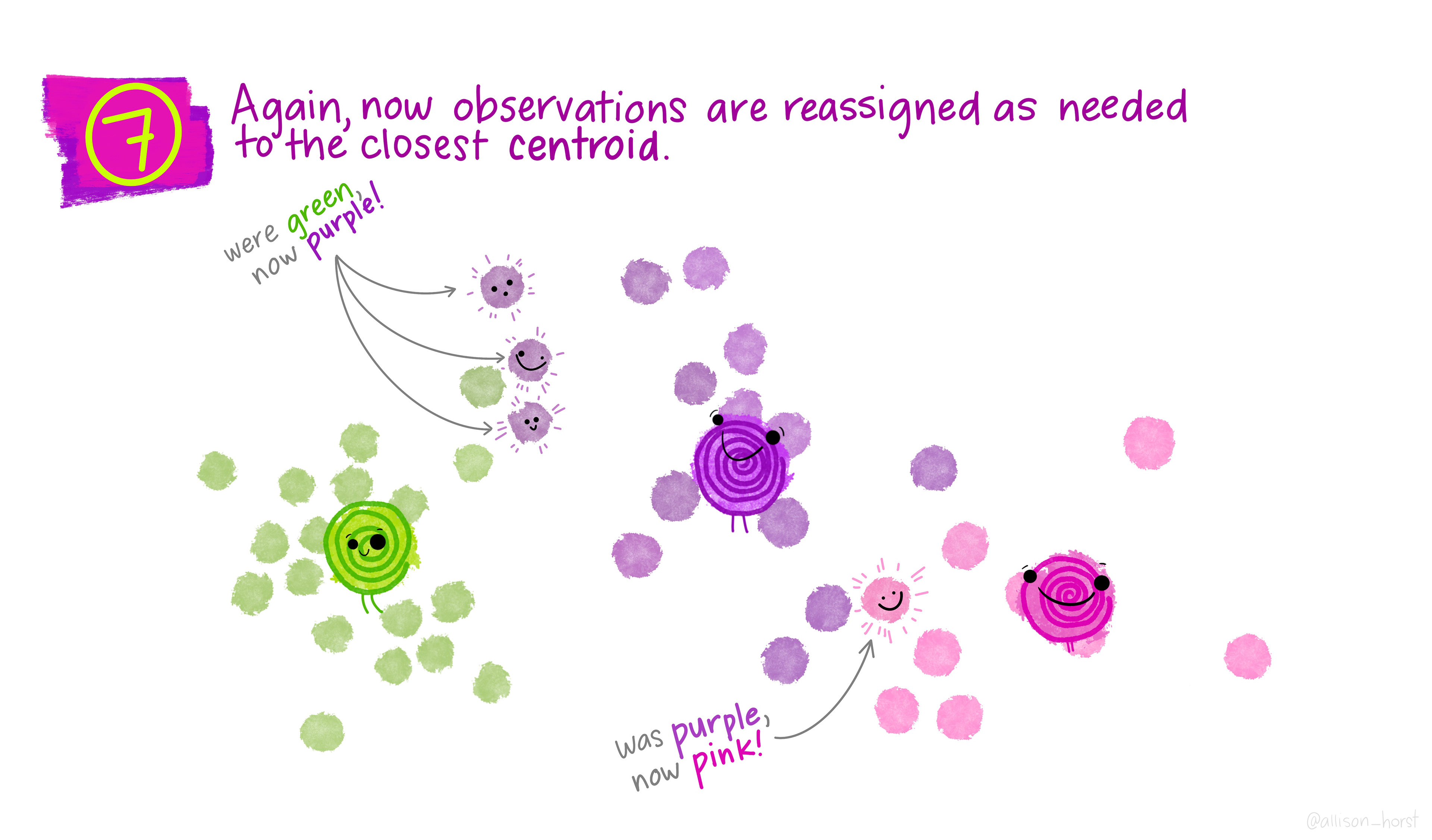
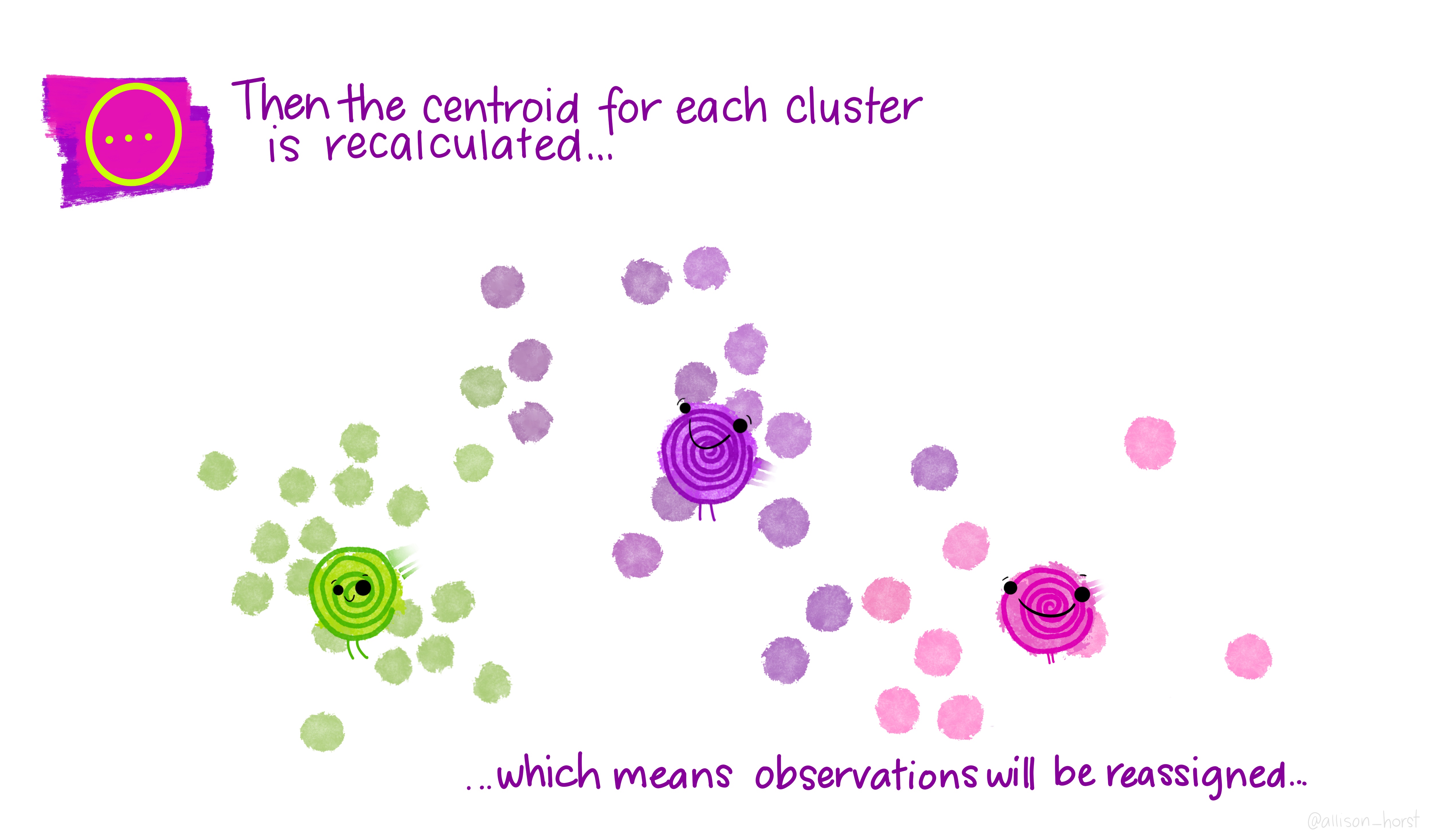
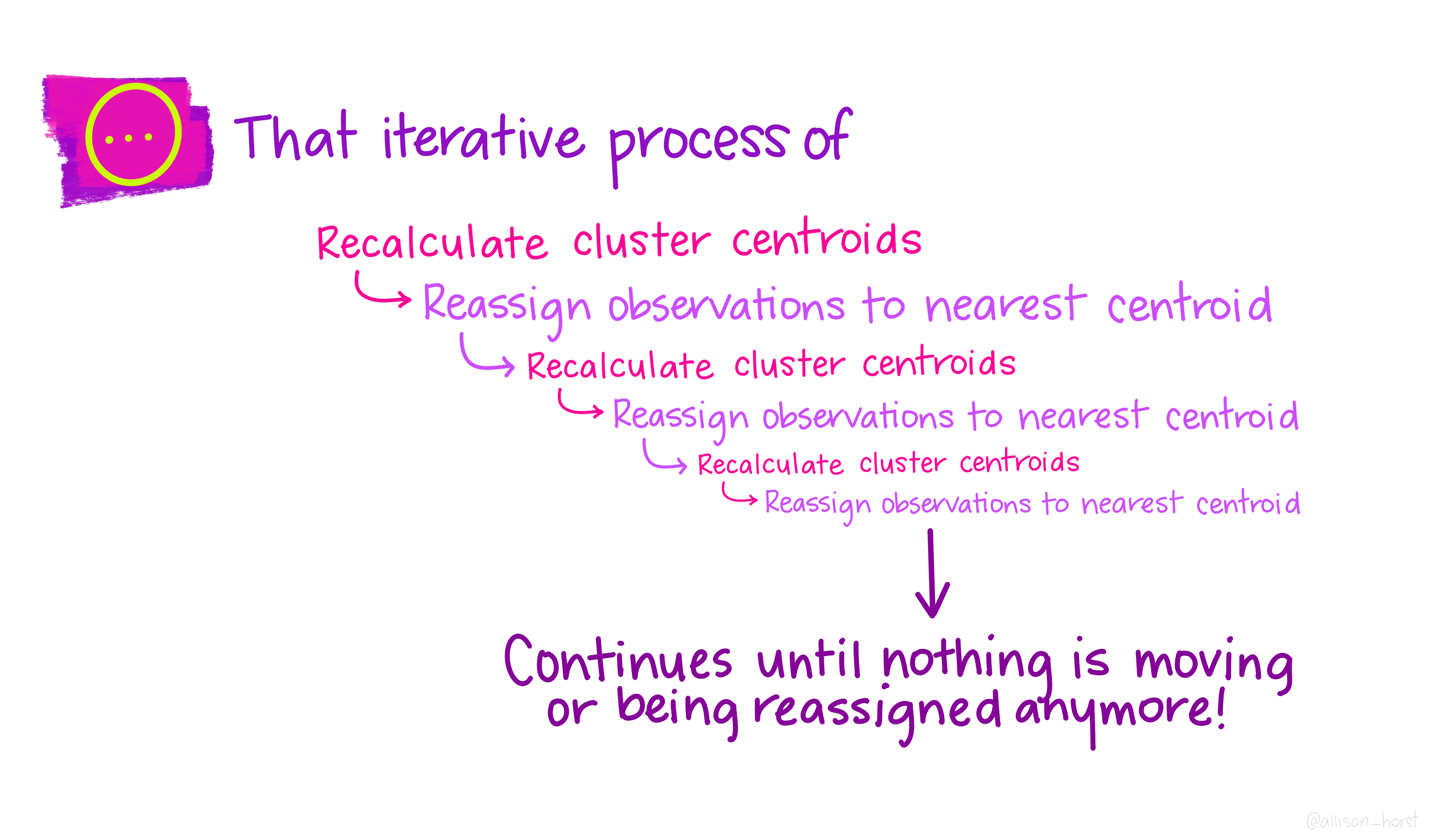
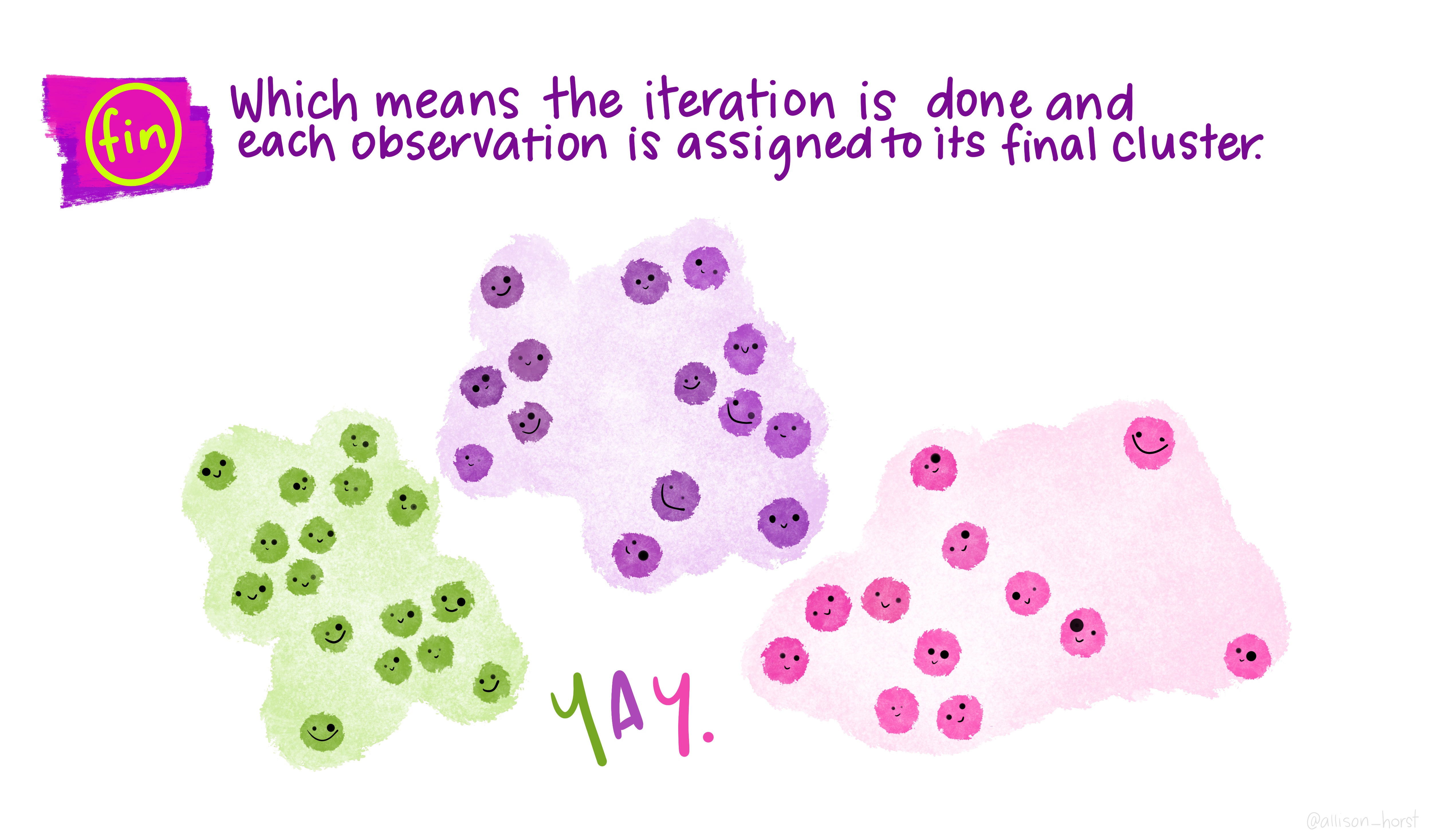
An overview of existing clustering algorithms
- For an overview of the clustering algorithms, their pros and cons and how they compare to each other, please head to (scikit-learn 2023a)
- For a comparison of clustering algorithms on toy datasets (with Python implementation), see (scikit-learn 2023b)
Clustering and anomaly detection in action
Demo on development indices (original data and R analysis in this post).
For the dataset, click on this button:
To download the indicators description, click on this button:
For clustering/anomaly detection demo notebook, click on this button:
Key concepts:
- Elbow method:
- method used to find the optimal number of clusters
- idea: to test various values of \(k\) and compute the within-cluster sum of squares (WCSS) for each of them, i.e the sum of square distances between the centroids and each point in the cluster and plot the graph \(k\) versus WCSS
- The WCSS is highest when \(k=1\) but decreases as \(k\) increases. The optimal \(k\) is reached where the graph starts to look like a straight line (i.e the elbow)
Alternative k-means initialization methods e.g k-means++ (see (Arthur and Vassilvitskii 2007)):
Basic idea of kmeans++ is selecting the first centroid randomly then assigning the remaining centroids based on the maximum squared distance: the goal is to push the centroids as far as possible from one another.
Here is the detailed K-means++ initialization algorithm:
- Assign \(c_1\) randomly (\(c_1\) being the first centroid)
- Calculate the distance between all data points and the selected centroid to get \(D_i=\max_{j\in[1,k]} ||x_i-c_j||^2\) (i.e the distance of a data point \(x_i\) from the farthest centroid \(c_j\)).
- Initialize the data point \(x_i\) as the next new centroid
- Repeat steps 2 and 3 till all the defined \(K\) centroids are found
Clustering and anomaly detection in action
A quick note on anomaly detection
- Aim: detect abnormal patterns in the data
- Based on the notions of similarity/density we discussed previously, can you guess how this goal is accomplished?
- Clustering is a useful tool here as well: anomalies are points that are farthest from any other or points that lie in areas of low density (refer to the same demo as in the previous slide to see how the DBSCAN algorithm - a clustering algorithm - is used for anomaly detection)
- To find out more about the DBSCAN algorithm mentioned in the demo, you can head here.
- You can also have a look at how anomaly detection is used in the context of credit card fraud here
What is unstructured data
Unstructured data is any type of data that lacks pre-defined formats and organization.
Structured data is collected following a known method or instance with a known schema (i.e table format), and unstructured data is everything else.
Unstructured data includes:
- Audio
- Video
- Text content, often unformatted for structured data collection, including text messages, emails, social media, business documents and news
Unstructured data is reusable:
- one piece of unstructured data can be examined different ways
- the person collecting the data does not have to define ahead of time what information needs to be collected from it
Because unstructured data can be used to satisfy multiple intentions, this could raise potential privacy concerns for the user
Analysing a book from Project Gutenberg: a case study
Project Gutenberg is a library of over 70,000 full texts of books or individual stories in the public domain.
We are going to explore a few key text mining concepts by downloading and processing a book from your choice out of that library. Head to the course website to download the notebook (Project Gutenberg case study materials) to follow along this part.
A few key definitions
Tokenization:
- The process of tokenization consists in splitting text into smaller units called tokens (most often words or sentences). In our case study, we split our text into words.
Lemmatization:
- The process of lemmatization groups together all inflections/variants of a word into a single form to more easily analyze each word. For instance, if you lemmatize “program”, “programming”, and “programmed” they would all be converted to “program”. This makes certain types of analysis much easier.
Stopwords:
- Stopwords are the words in any language which does not add much meaning to a sentence. They can safely be ignored without sacrificing the meaning of the sentence. They tend to be the most common words in the language (e.g in English “a”, “the”, “is”, “are”, etc.) but can also be task-specific (e.g the word “immigration” in a corpus entirely about the topic of immigration).
Analysing the news: a case study
We use the newspaper3k package from Python to extract the most recent UK-related news articles from several newspapers:
- The Guardian
- BBC
- The Sun
- The Telegraph
- The Independent
- The Financial Times
Head to the course website to download the material needed to follow this second demo (news case study materials).
Introducing the concept of corpus
What is a corpus?
- Simply put, a corpus is a collection of texts. It can be monolingual or multilingual.
- The plural of corpus is corpora.
- You can find some examples of publicly available (downloadable) corpora here.
The concept of Term frequency-inverse document frequency (TF-IDF)
- Text vectorizer method that transforms the text into a usable vector i.e assigns a number to words in a text
- Each number is a function of the word (term) frequency and inverse document frequency:
- term frequency (TF) is how often a word appears in a document, divided by how many words there are. Term frequency measures how common a word is.
- inverse document frequency (IDF) is how unique or rare a word is and is: \(IDF(t) = log_e(\textrm{Total number of documents} / \textrm{Number of documents with term t in it})\)
Example:
Consider a document containing 100 words where the word cooker appears 5 times. The term frequency (i.e., TF) for cooker is then (5 / 100) = 0.05.
Now, assume we have 10 million documents and the word cooker appears in one thousand of these. Then, the inverse document frequency (i.e., IDF) is calculated as log(10,000,000 / 1,000) = 4.
Therefore, the TF-IDF weight is the product of these quantities: 0.05 * 4 = 0.20.
To learn more about TF-IDF, see this link or this one
Once vectorized, the text can be used as input to ML algorithms (supervised or unsupervised)!
Other Python libraries for NLP
References

LSE DS101 2024/25 Autumn Term
