🗓️ Week 08
Machine Learning II

DS101 – Fundamentals of Data Science

Dr. Ghita Berrada

LSE Data Science Institute

18 Nov 2024

What we will cover today:

• Some more exploration of supervised learning
• And now for unsupervised learning

Some more exploration of supervised learning

The Decision Tree model

The Decision Tree model applied to diabetes: the metrics

       precision    recall  f1-score   support

    Negative       0.83      0.98      0.90        54
    Positive       0.99      0.89      0.94       102

    accuracy                           0.92       156
   macro avg       0.91      0.94      0.92       156
weighted avg       0.93      0.92      0.92       156

The Support Vector Machine model

The Support Vector Machine model

Say you have a dataset with two classes of points:

The Support Vector Machine model

The goal is to find a line that separates the two classes of points:

The Support Vector Machine model

It can get more complicated than just a line:

• Explain the dataset

Neural Networks

Deep Learning

• Stack a lot of layers on top of each other, and you get a deep neural network.
• Forget about interpretability!

Attention

• The Transformer architecture is a deep learning model that uses attention to learn contextual relationships between words in a text.
• It has revolutionized the field of Natural Language Processing (NLP).

And now for unsupervised learning

Types of Machine Learning

Supervised
Learning

• Each data point is associated with a label.
• The goal is to learn a function that maps the data to the labels.

(🗓️ Week 07)

Unsupervised
Learning

• There is no such association between the data and the labels.
• The focus is on similarities between data points.

(🗓️ Week 08)

What is Unsupervised Learning

Unsupervised learning algorithms :

• rely on unlabeled data
• learn hidden patterns in the data without human intervention

Types of Unsupervised Learning

Clustering

• Consists in dividing data points into clusters, i.e groups of points that are similar between themselves and are dissimilar to data points belonging to other cluster
• Examples:
  • segmenting patients with a particular condition (e.g cancer) into groups depending on their response to particular treatment drugs (aim: treatment personalisation)
  • customer segmentation according to common traits and/purchasing behaviour (aim: guiding marketing and business strategies)

Association rule mining

• Series of algorithms that try to find rules to discover the probability of the co-occurrence of items in a collection
• E.g:
  • Given a collection of supermarket purchase records/transactions, can we tell how likely a customer is to buy milk if he/she has bought bread?
  • Can we learn how likely a series of medical diagnoses are, given the symptoms to which they are associated?

Types of Unsupervised Learning

Dimensionality reduction

• Techniques that reduce the number of features, or dimensions, in a dataset (prior to applying a classification or regression algorithm)
• Most commonly known techniques: Principal Component Analysis (PCA), Singular Value Decomposition (SVD), t-SNE, UMAP
• See this video to get some explanation about PCA

Anomaly detection

• Techniques that discover unusual data points in a dataset i.e with patterns that deviate from normal dataset patterns
• E.g:
  • Fraud detection (credit card fraud)
  • Cyberattack detection
  • Also useful in predicting whether a patient has or doesn’t have a disease

Unsupervised learning: where is it used in practice?

• Market Basket Analysis : The goal here is to understand customer purchasing patterns and it involves analyzing data, e.g purchase history, to reveal product groupings and products likely to be purchased together.
• Recommendation engines: Using data such as past purchasing or browsing behaviour or past product/services ratings or behaviour of similar users, unsupervised learning algorithms are used to suggest products, services, information to a user might like or find interesting
• Medical imaging: Unsupervised learning algorithms are used for tasks as essential in radiology and pathology to diagnose patients quickly and accurately as image detection, classification and segmentation
• Computer vision: Visual perception tasks such as object recognition rely on unsupervised learning algorithms
• Natural language processing (NLP): Google News uses unsupervised learning to categorize articles based on the same story from various news outlets; for example, the results of the football transfer window would all be categorized under football.
• Anomaly detection: The idea is to find atypical patterns in the data, i.e anomalies. Anomalies can be anything from a disease/medical diagnosis, a pattern of fraud (e. credit card fraud, insurance fraud, money laundering), security breaches (e.g cyberattacks) or faulty equipment
• Genetic research: Clustering algorithms, in particular hierarchical clustering, are often used to analyze DNA patterns and reveal evolutionary relationships.

Similarity

• Notion central to clustering and anomaly detection
• Quantifies how data samples are related or close to each other
• Often expressed as a number between 0 and 1
• The higher it is, the closer the points are together, i.e “the more similar” they are
• Based on a distance function

Similarity

Examples of common distance/similarity functions:

Real-valued data:

• Euclidian distance: \(d(A,B)=\sqrt{\sum_{i=1}^n |A_i-B_i|^2}\)

• Cosine distance: \(S_C(A,B)=\frac{\sum_{i=1}^n A_iB_i}{\sqrt{\sum_{i=1}^n A_i^2}\sqrt{\sum_{i=1}^n B_i^2}}\)

where A and B are two n-dimensional vectors of attributes, and \(A_i\) and \(B_i\) the \(i\)th components of vectors A and B respectively

String similarity:

• Hamming distance: given two strings of equal length, it is the number of positions at which the corresponding symbols (i.e either letters, bits, or decimal digits) are different e.g:
  • 0000 and 1111 is 4
  • cat and car is 1
  • call and cold is 2

Similarity

Examples of common distance/similarity functions:

String similarity

• Levenstein distance: given two strings, it’s the minimal number of edits (substutions, deletions, insertions) needed to turn one string into another e.g:

  The Levenshtein distance between kitten and sitting is 3, since the following 3 edits change one into the other, and there is no way to do it with fewer than 3 edits:

  1. kitten → sitten (substitution of “s” for “k”),
  2. sitten → sittin (substitution of “i” for “e”),
  3. sittin → sitting (insertion of “g” at the end).

Set similarity:

A set is a collection of items with no order or repetition. Sets are typically used to represent relationships or associations between objects or even people.

• Jaccard index: it is often used in recommendation systems and social media analysis and measures the similarity between two sets based on the number of items present in both sets relative to the total number of items
  \(J(A,B)=\frac{|A\cap B|}{|A\cup B|}\)
  where A and B are two sets, \(|A\cap B|\) the number of items included in both sets and \(|A\cup B|\) the total number of items

Density

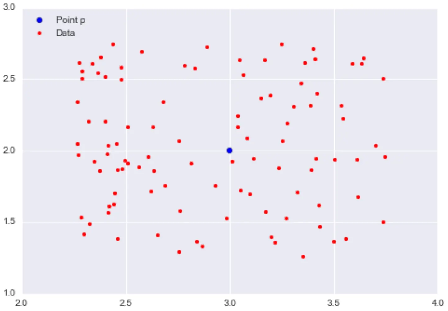
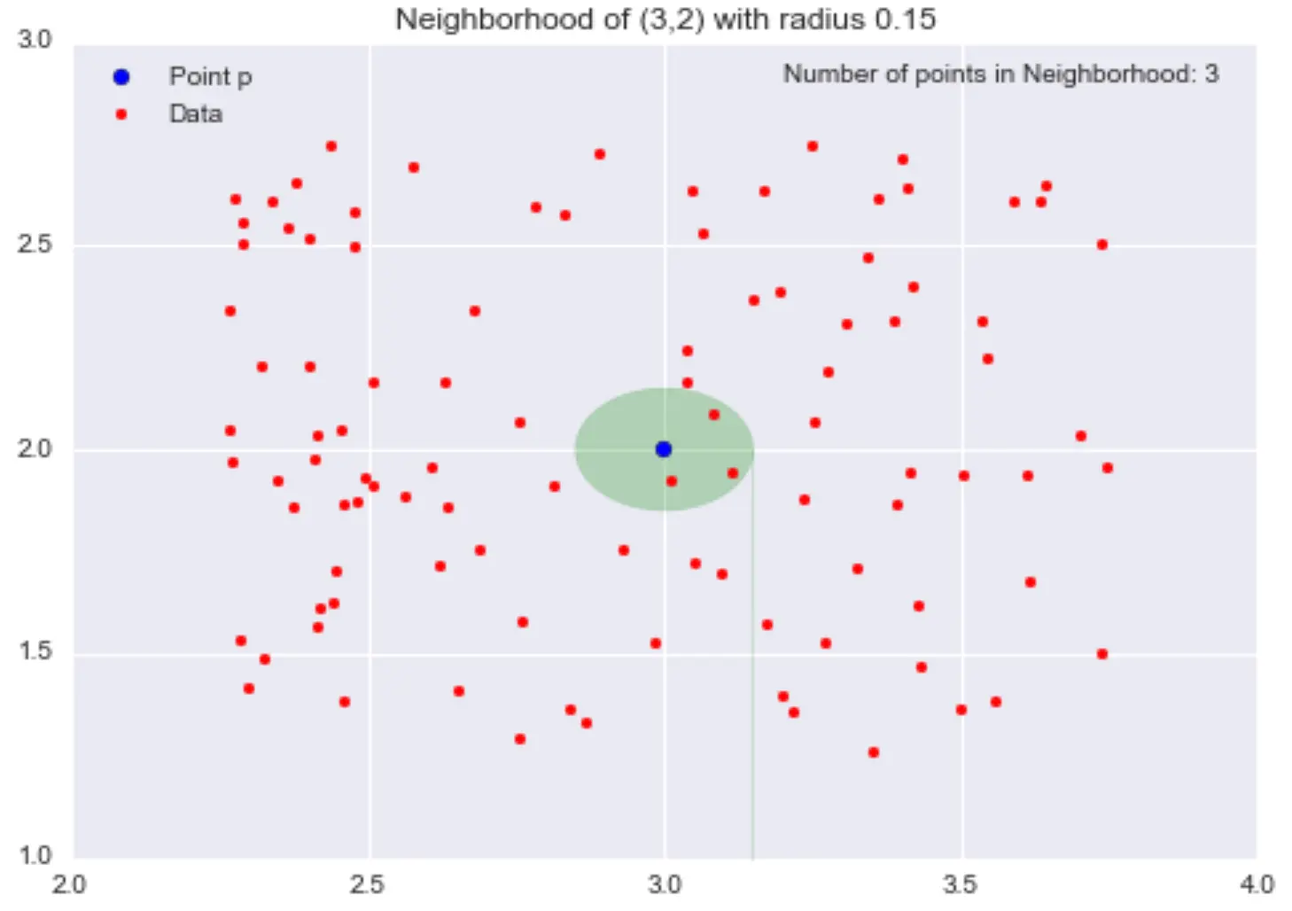
\(\epsilon\)-neighbourhoods:

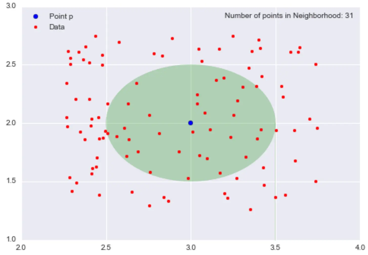
• given \(\epsilon>0\) and a point \(p\), the \(\epsilon\)-neighbourhood of \(p\) is the set of points that are at distance at most \(\epsilon\) away from \(p\)

Example:
(Images source: https://domino.ai/blog/topology-and-density-based-clustering)

100 points scattered on the [1,3]x[2,4] grid. We pick (3,2) as our point \(p\)

We draw the neighbourhood of \(p\) with radius \(\epsilon=0.5\): 31 points are in the neighbourhood

We draw the neighbourhood of \(p\) with radius \(\epsilon=0.15\): 3 points are in the neighbourhood

Density (continued)

Density:

• Roughly defined, \(\textrm{density}=\frac{\textrm{"mass"}}{\textrm{"volume"}}\)
• If we go back to our previous example, the “mass” would be the number of points in an \(\epsilon\)-neighbourhood centered in \(p\) and the “volume” the area of radius \(\epsilon\) centered around \(p\)

Example:

If we take the figure above, the local density estimation at \(p=(3,2)\) is \(\frac{31}{0.25\pi} \approx 39.5\)

• Number that is meaningless on its own
• If we calculate the densities of all points in our dataset, we could say that points within the same neighbourhood and similar local densities belong to the same cluster \(\rightarrow\) General principle of density-based clustering methods e.g DBSCAN (see (Ester et al. 1996) for more details on the DBSCAN algorithm)

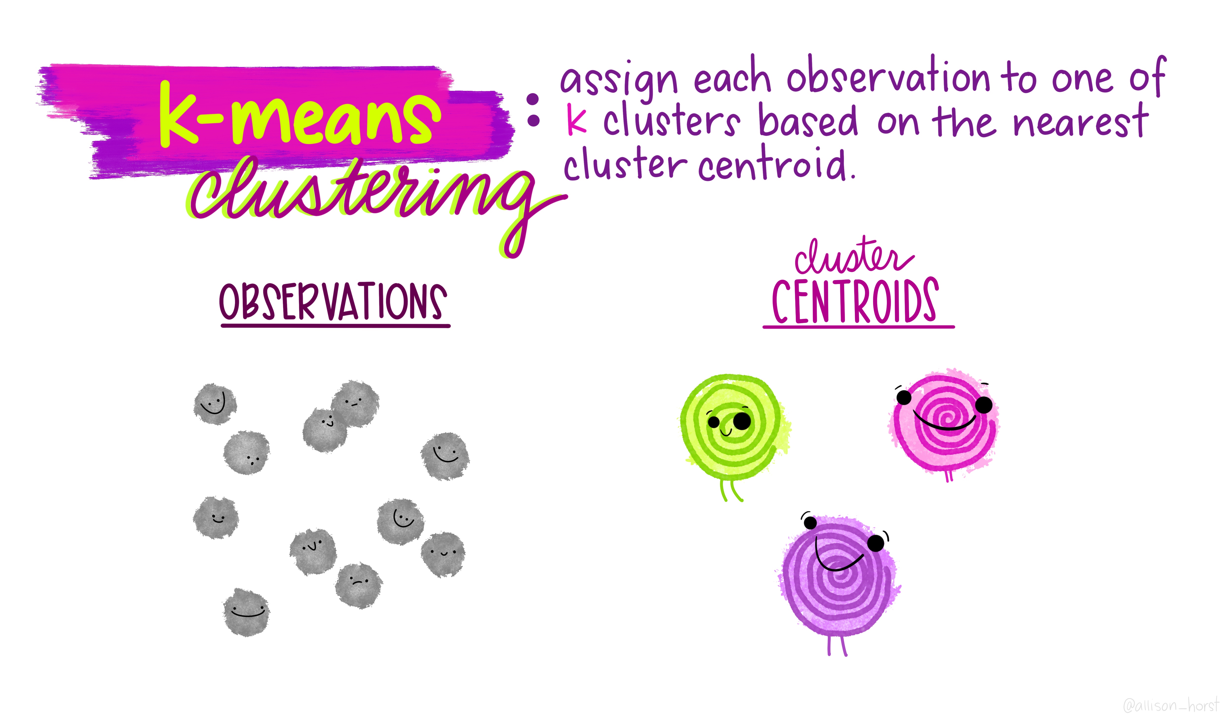
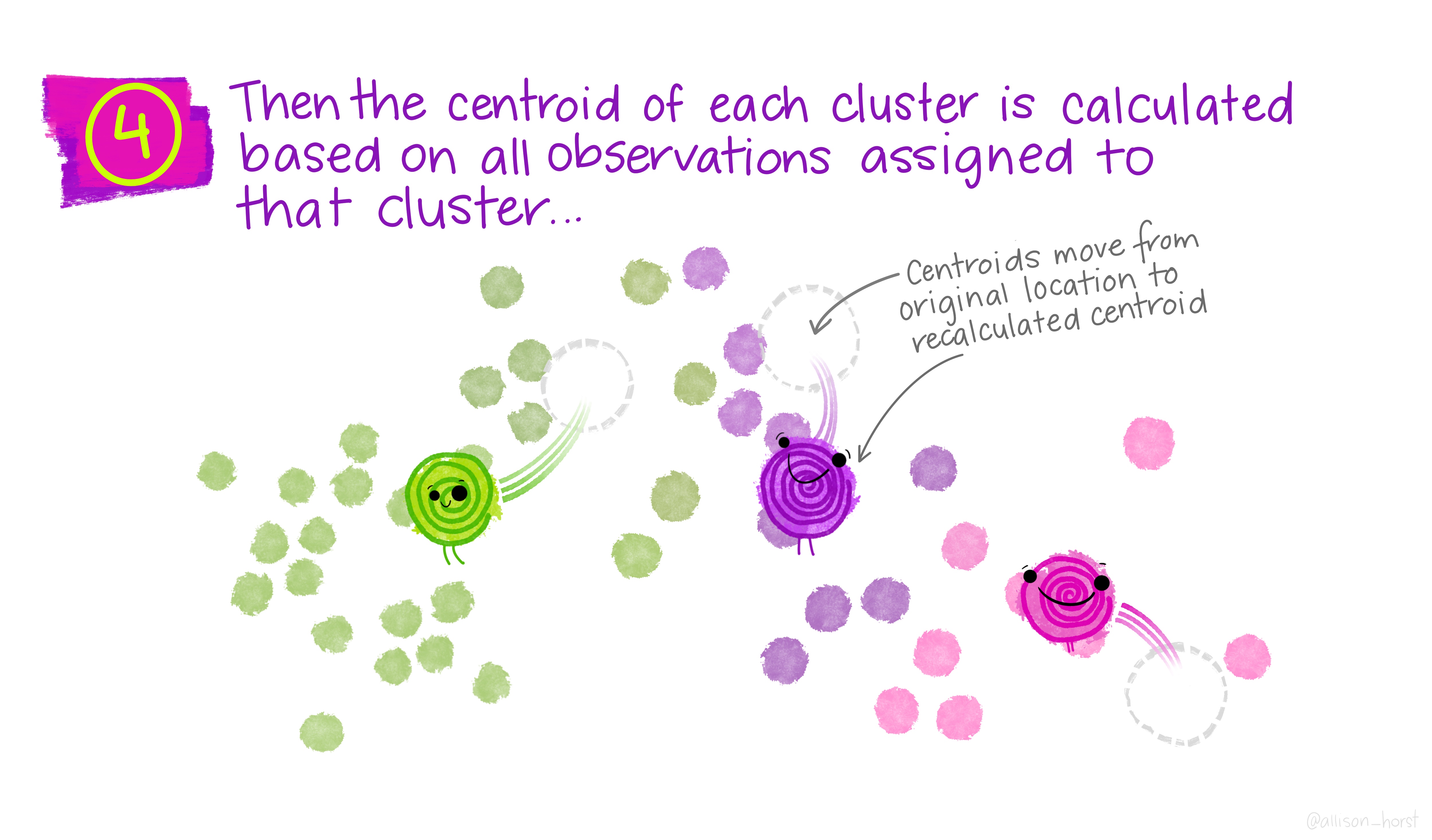
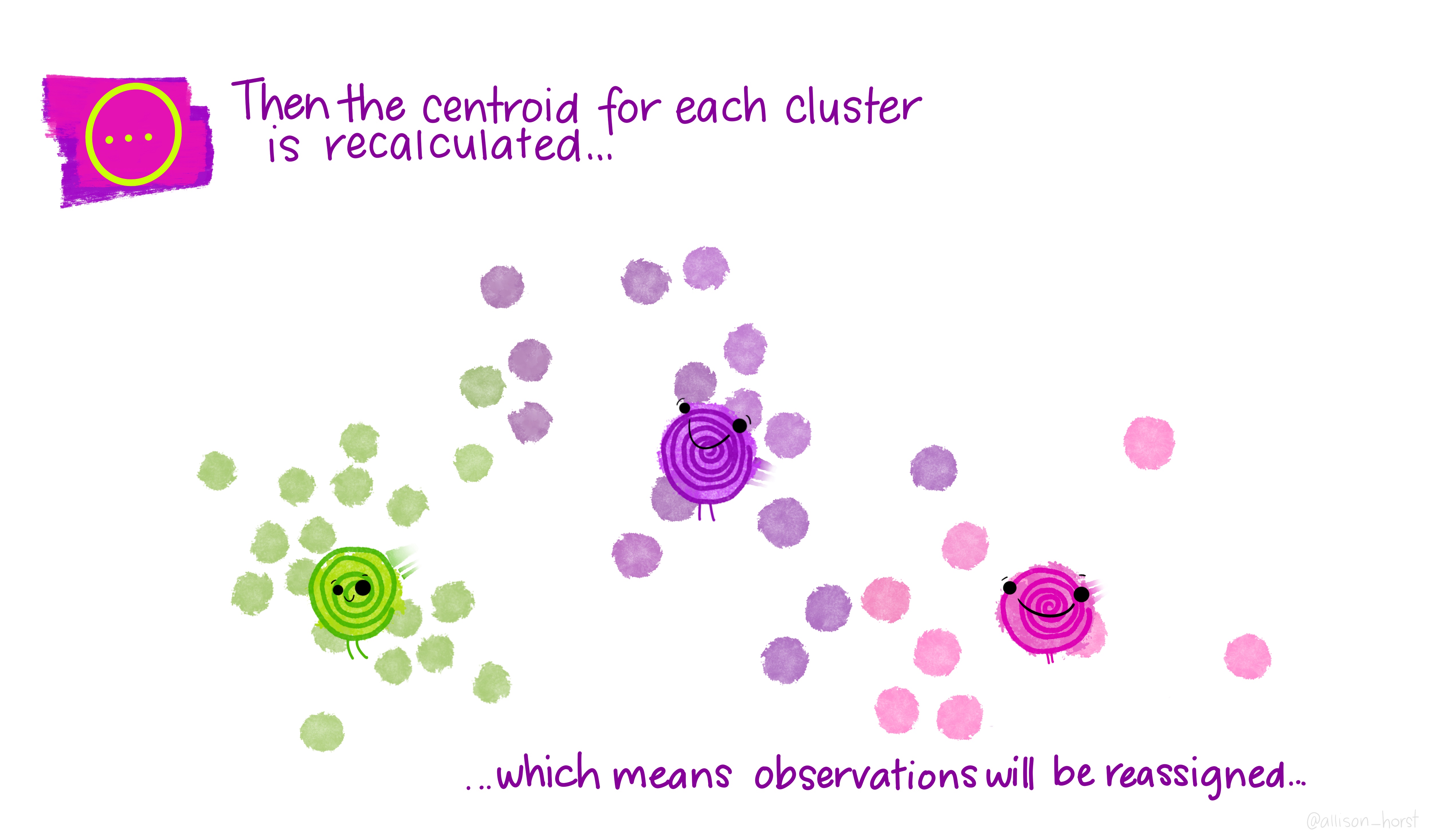
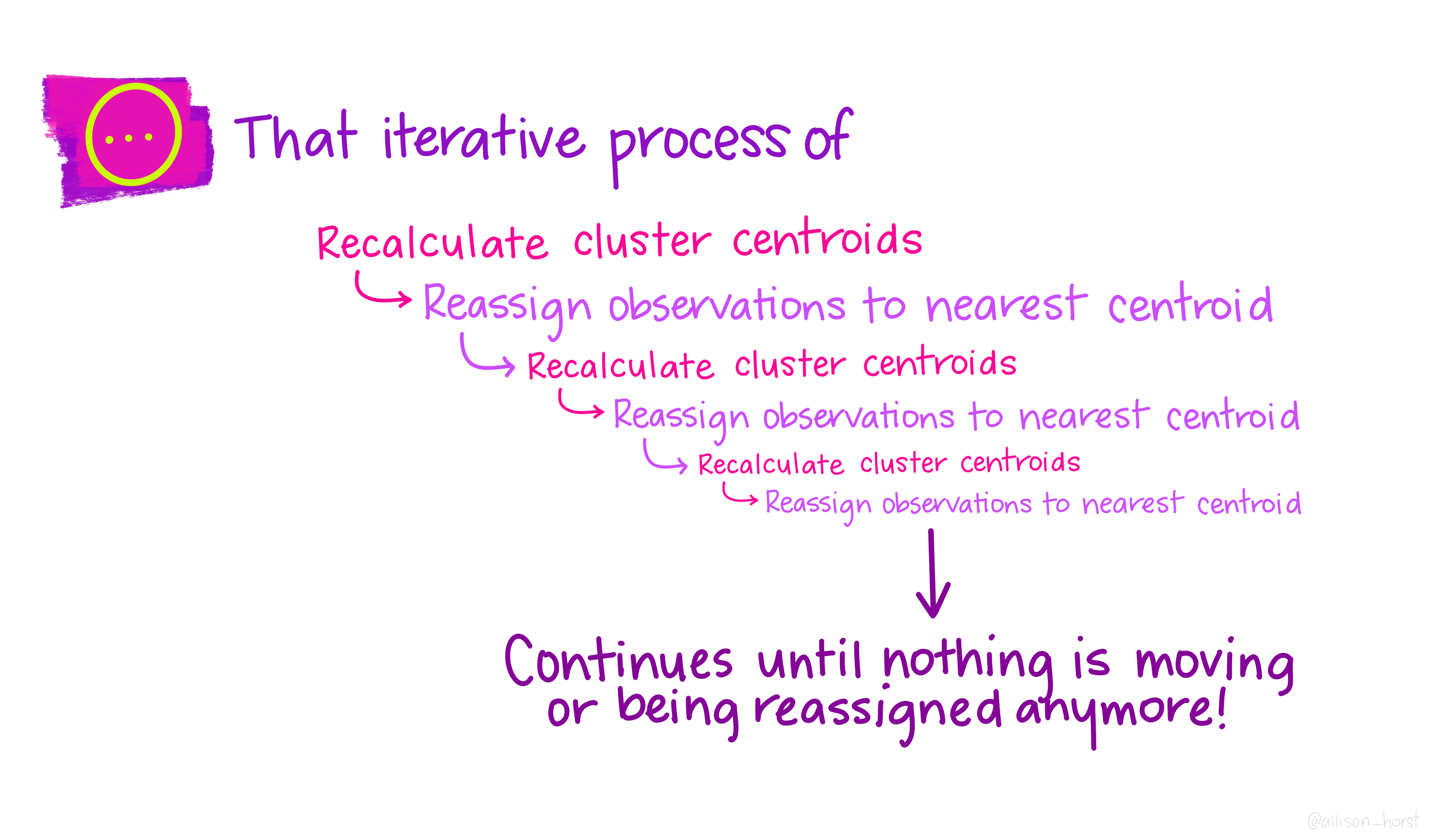
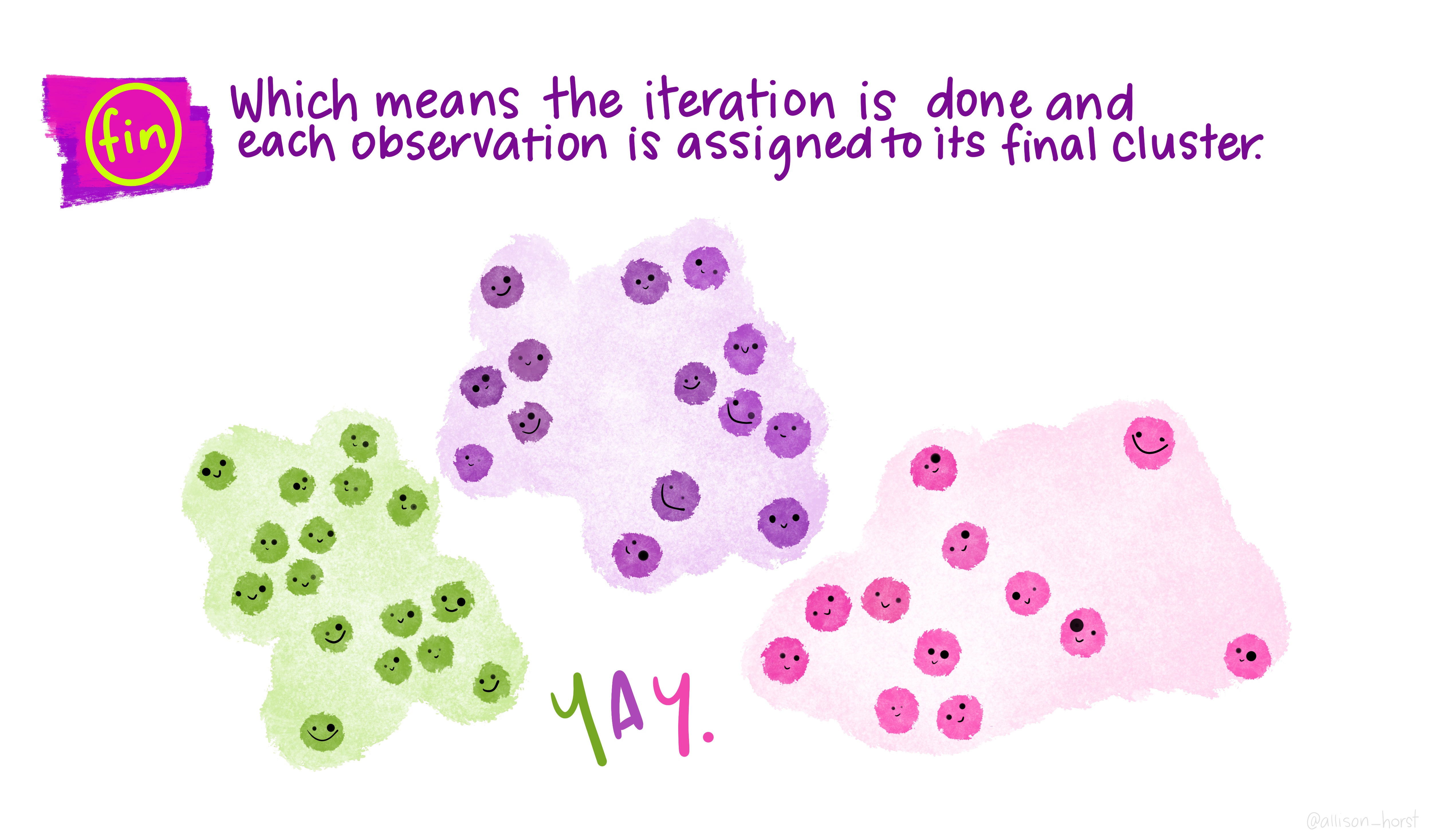
An example of clustering algorithm: k-means

Artwork by @allison_horst

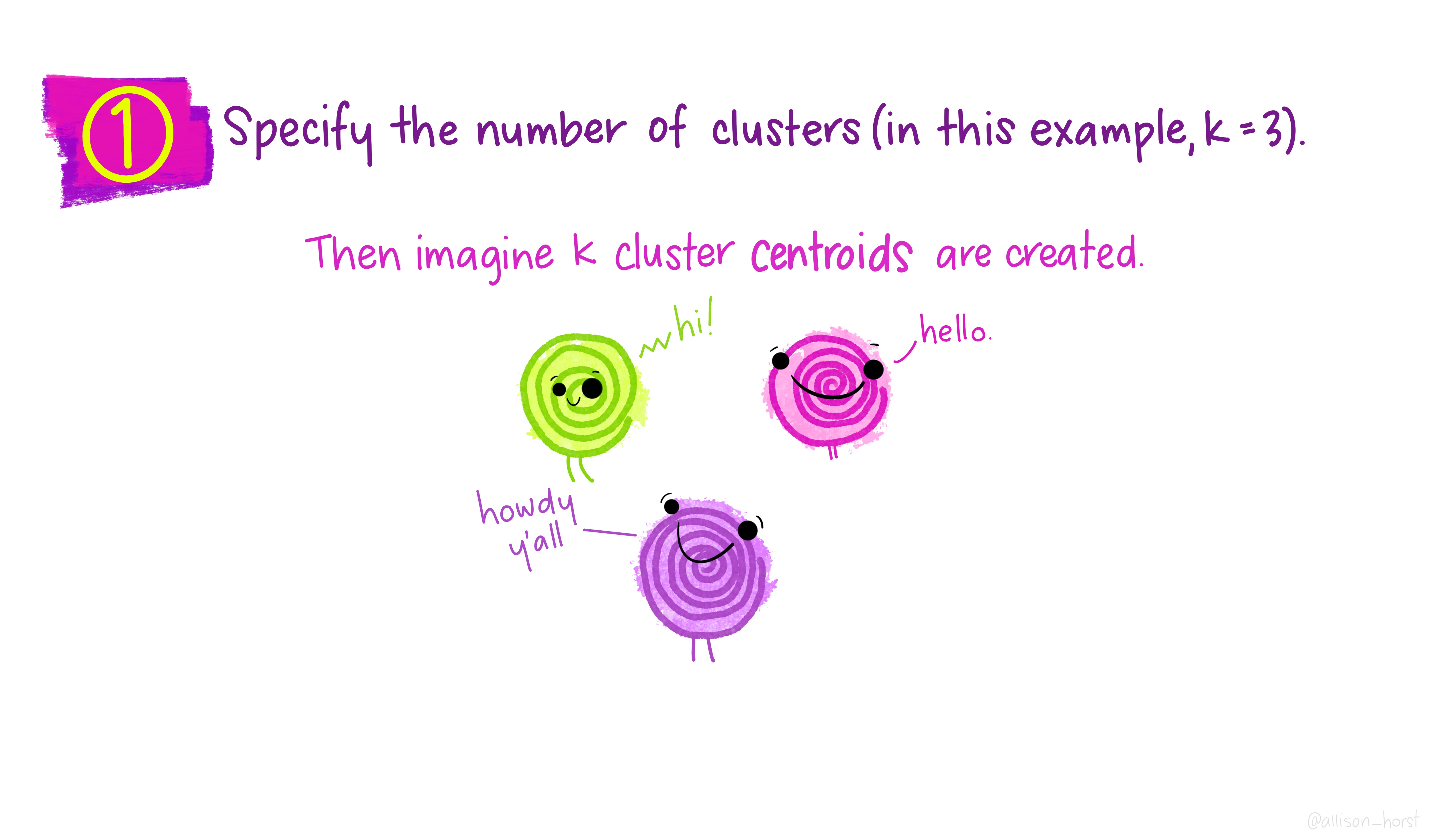
An example of clustering algorithm: k-means (continued)

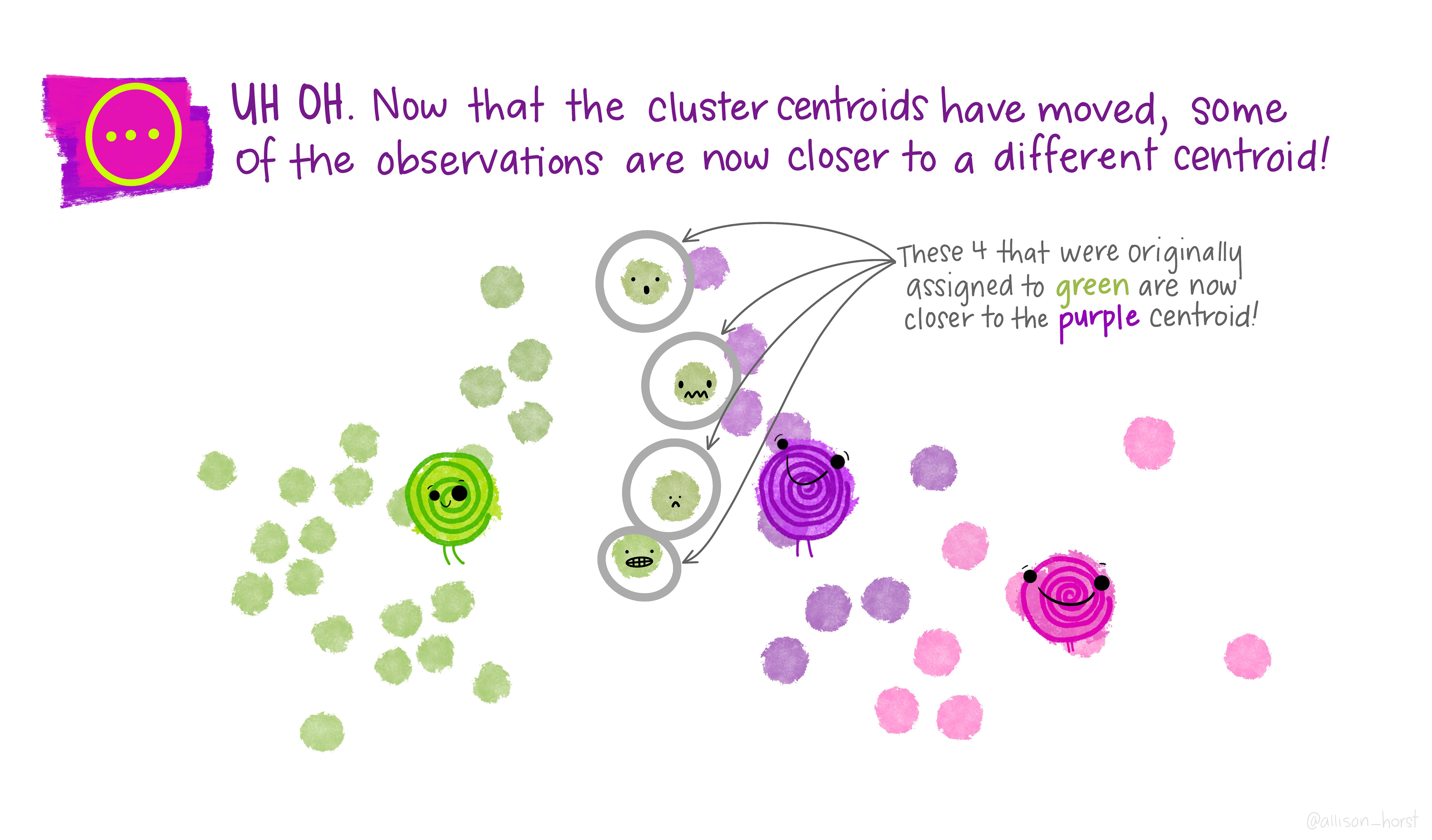
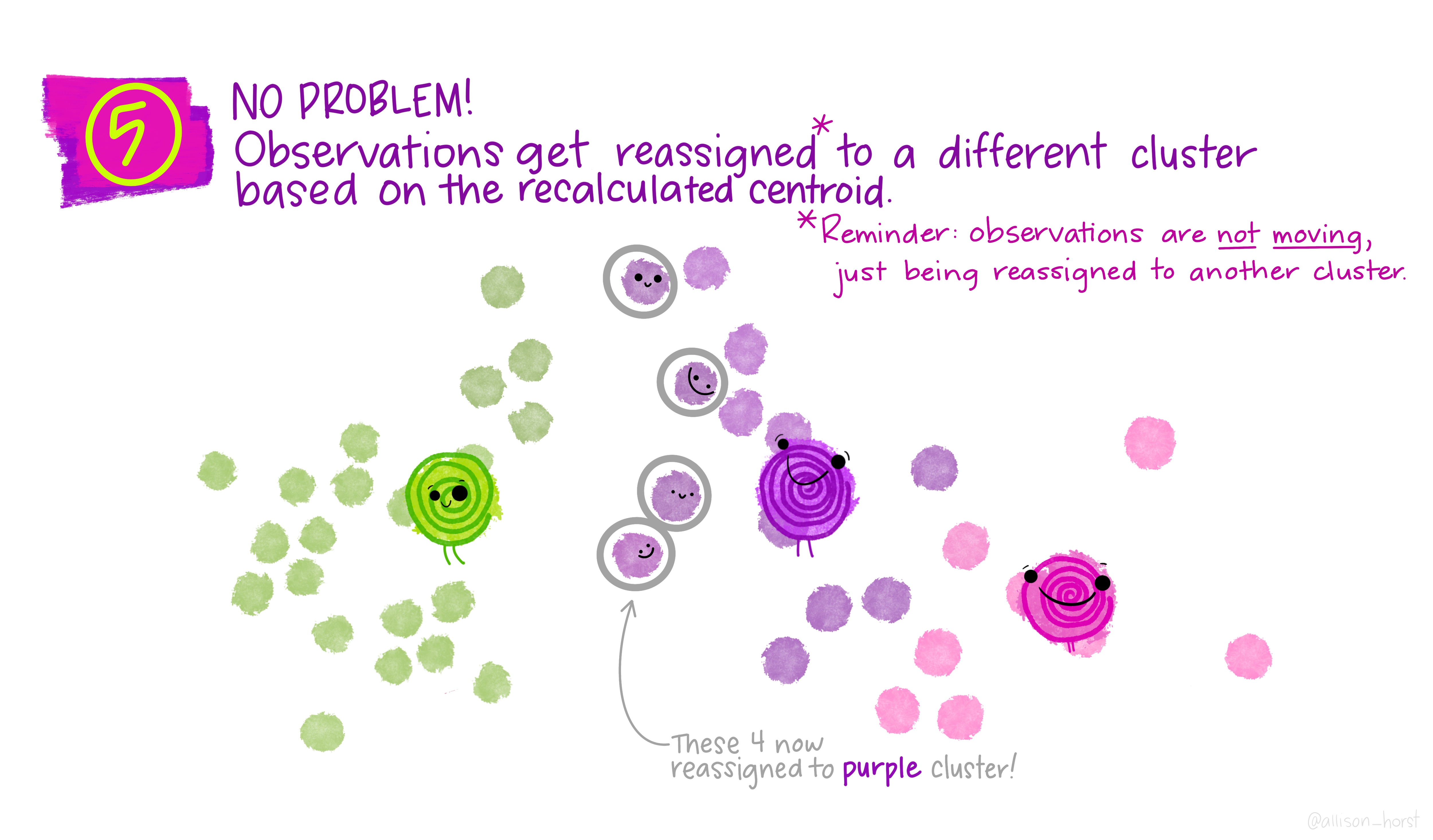
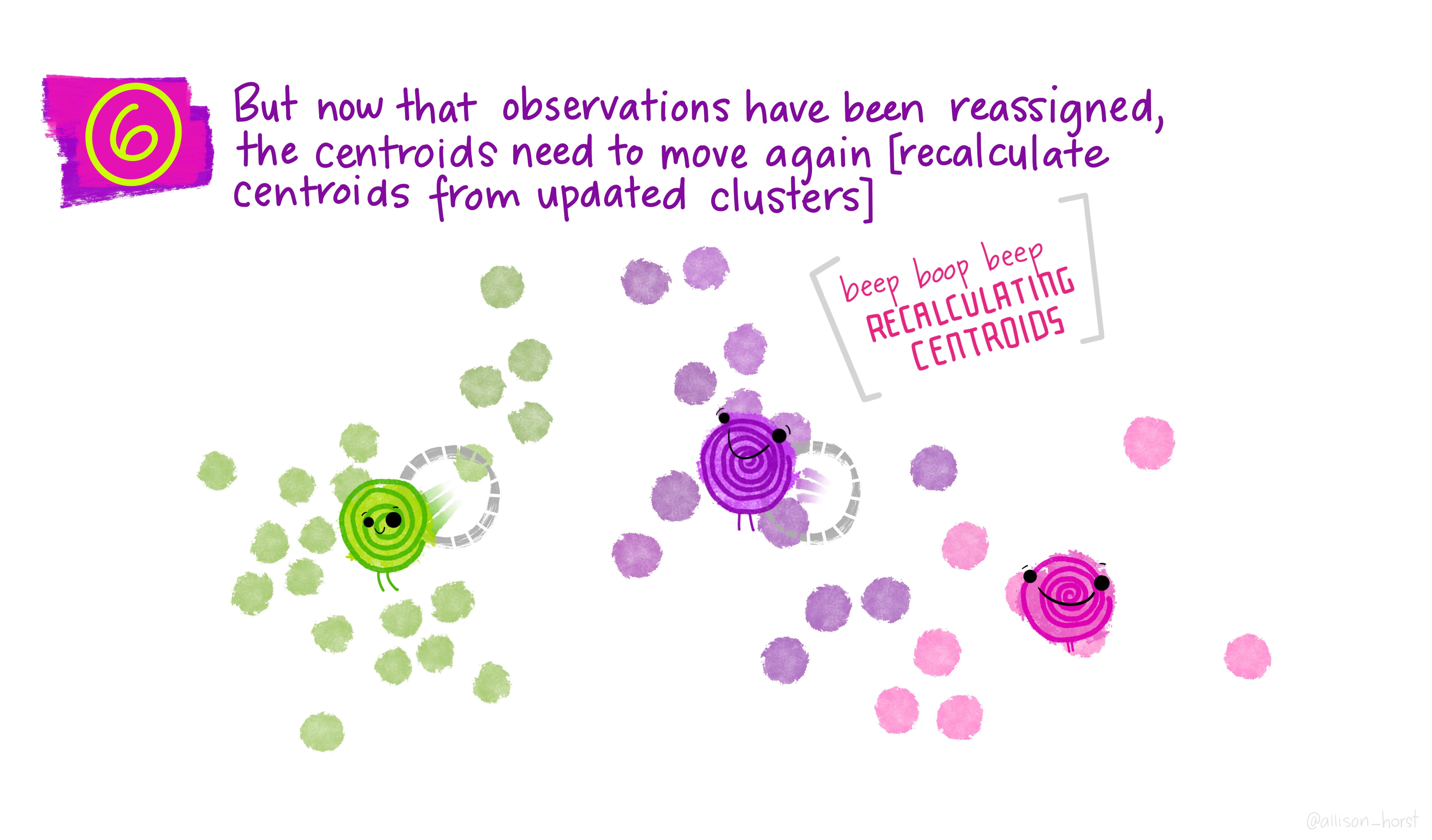
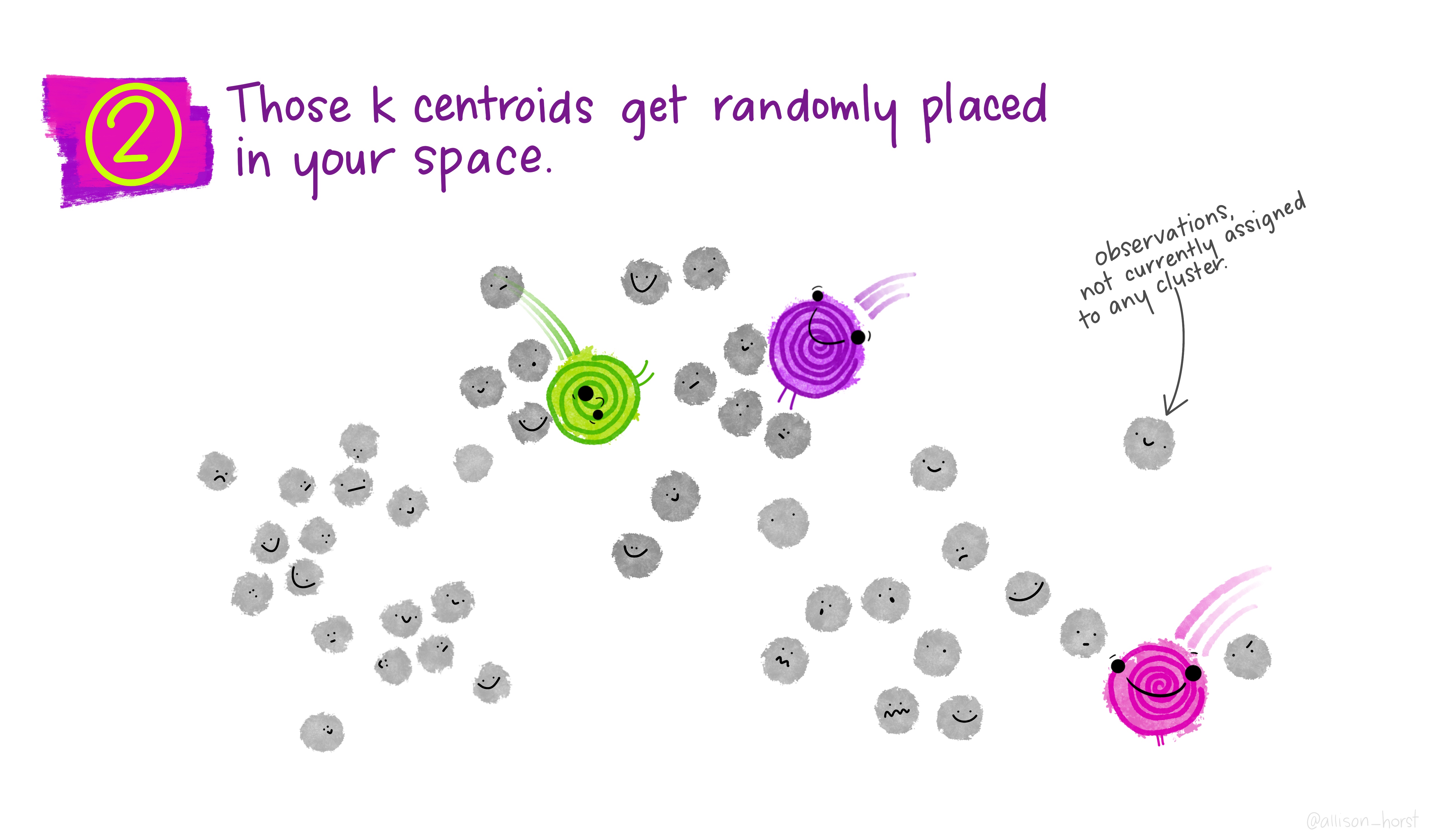
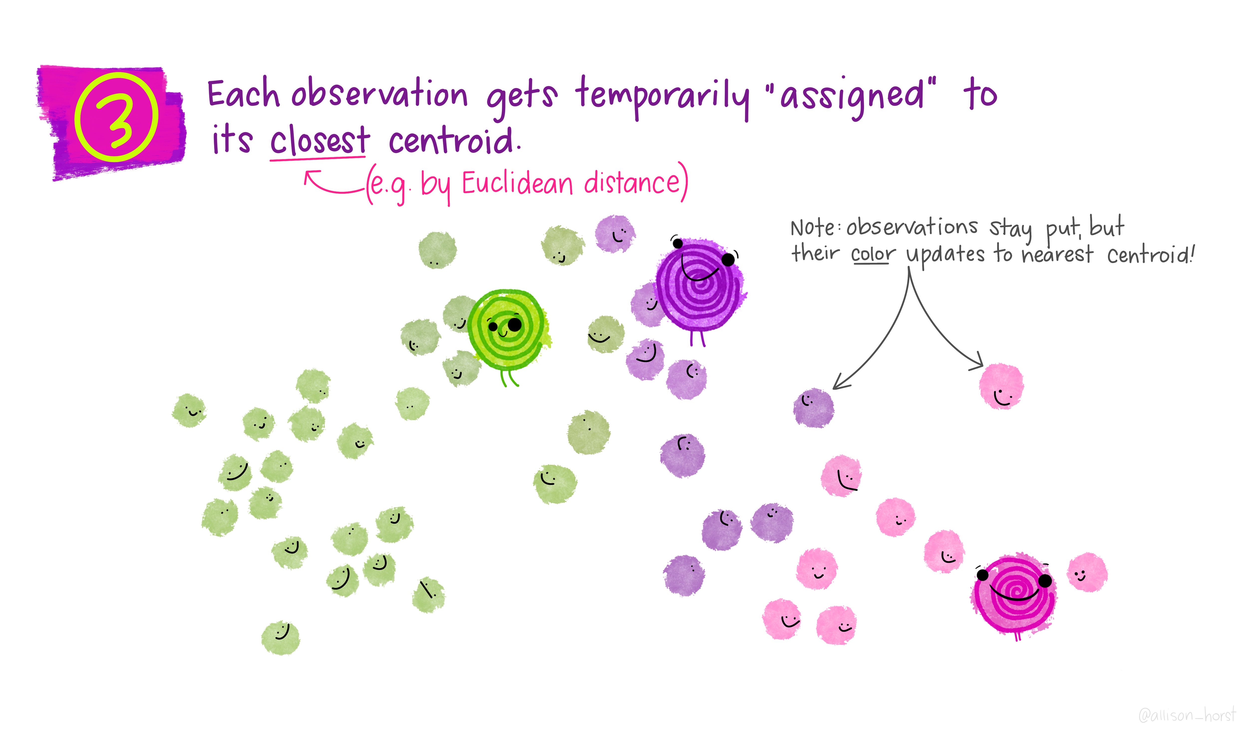
An example of clustering algorithm: k-means (continued)

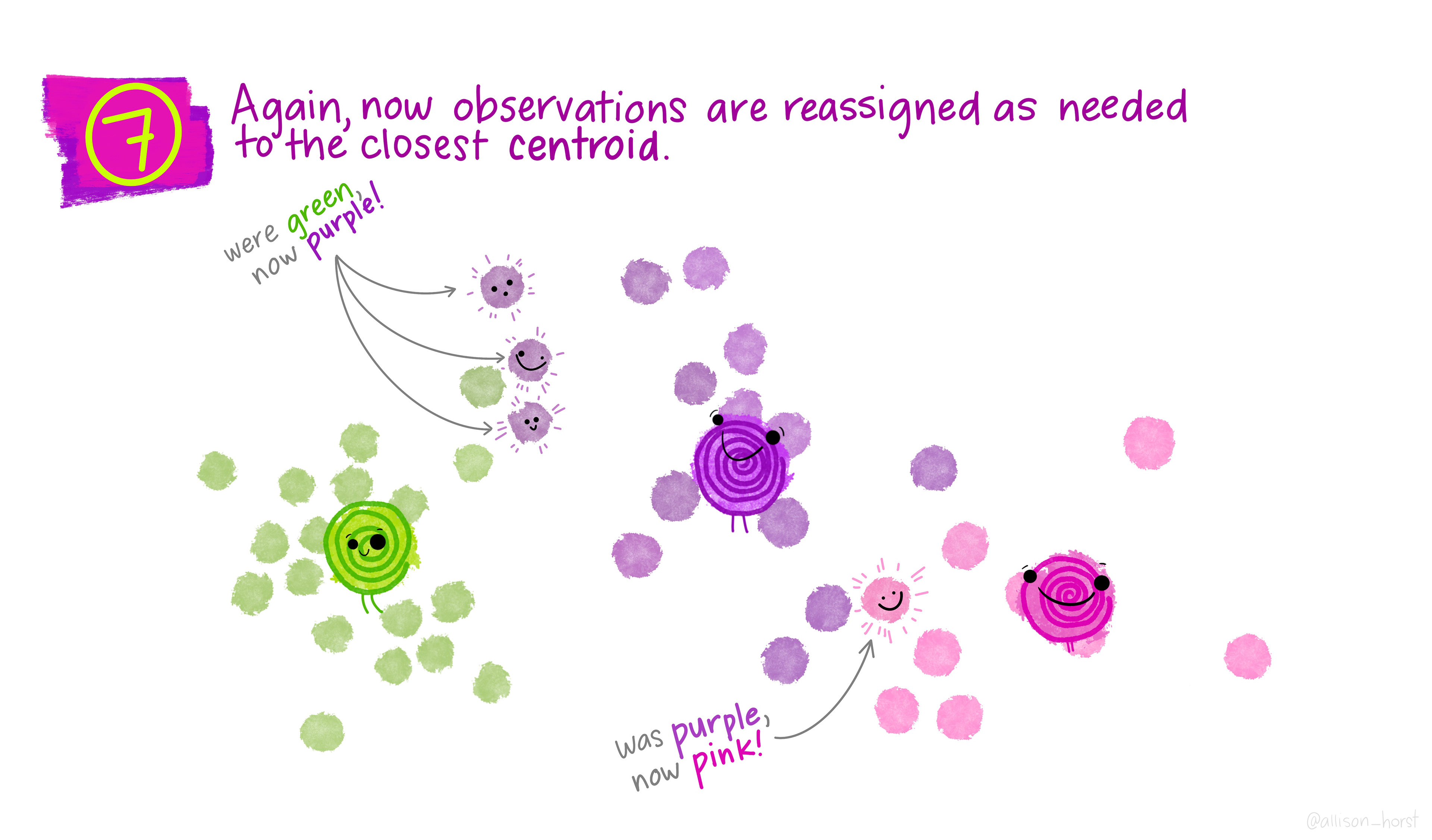
An overview of existing clustering algorithms

• For an overview of the clustering algorithms, their pros and cons and how they compare to each other, please head to (scikit-learn 2023a)
• For a comparison of clustering algorithms on toy datasets (with Python implementation), see (scikit-learn 2023b)

Time for a break 🍵

After the break:

• Clustering in practice
• Anomaly detection

Clustering in action: customer segmentation

Demo on Mall customer segmentation (original notebook and data from Kaggle):

• For the dataset, click on this button:
• For clustering demo notebook, click on this button:

Key concepts:

• Elbow method:
  • method used to find the optimal number of clusters
  • idea: to test various values of \(k\) and compute the within-cluster sum of squares (WCSS) for each of them, i.e the sum of square distances between the centroids and each point in the cluster and plot the graph \(k\) versus WCSS
  • The WCSS is highest when \(k=1\) but decreases as \(k\) increases. The optimal \(k\) is reached where the graph starts to look like a straight line (i.e the elbow)

• Alternative k-means initialization methods e.g k-means++ (see (Arthur and Vassilvitskii 2007)):

  Basic idea of kmeans++ is selecting the first centroid randomly then assigning the remaining centroids based on the maximum squared distance: the goal is to push the centroids as far as possible from one another.

  Here is the detailed K-means++ initialization algorithm:

  1. Assign \(c_1\) randomly (\(c_1\) being the first centroid)
  2. Calculate the distance between all data points and the selected centroid to get \(D_i=\max_{j\in[1,k]} ||x_i-c_j||^2\) (i.e the distance of a data point \(x_i\) from the farthest centroid \(c_j\)).
  3. Initialize the data point \(x_i\) as the next new centroid
  4. Repeat steps 2 and 3 till all the defined \(K\) centroids are found

Anomaly detection

• Aim: detect abnormal patterns in the data

• Based on the notions of similarity/density we discussed previously, can you guess how this goal is accomplished?

• Clustering is a useful tool here as well: anomalies are points that are farthest from any other or points that lie in areas of low density

• Quick demo using the same Mall customer dataset from earlier. To download the new demo notebook, click on this button:

• To find out more about the DBSCAN algorithm mentioned in the demo, you can head here.

• You can also have a look at how anomaly detection is used in the context of credit card fraud here

References

Arthur, David, and Sergei Vassilvitskii. 2007. “K-Means++ the Advantages of Careful Seeding.” In Proceedings of the Eighteenth Annual ACM-SIAM Symposium on Discrete Algorithms, 1027–35.

Ester, Martin, Hans-Peter Kriegel, Jörg Sander, and Xiaowei Xu. 1996. “A Density-Based Algorithm for Discovering Clusters in Large Spatial Databases with Noise.” In Proceedings of the Second International Conference on Knowledge Discovery and Data Mining, 226–31. KDD’96. Portland, Oregon: AAAI Press.

scikit-learn. 2023a. “Scikit Learn User Guide: Clustering.” Scikit-Learn. https://scikit-learn/stable/modules/clustering.html.

———. 2023b. “Scikit Learn User Guide: Comparing different clustering algorithms on toy datasets.” Scikit-Learn. https://scikit-learn.org/stable/auto_examples/cluster/plot_cluster_comparison.html.

References

LSE DS101 2024/25 Autumn Term