🗓️ Week 05
Statistical Inference II

DS101 – Fundamentals of Data Science

Dr. Ghita Berrada

LSE Data Science Institute

23 Oct 2023

What we will cover today:

• Building a statistical model
• Dependent variable
• Independent variables
• Now for something (slightly) different

Statistical Inference I & II

What we will talk about this week:

🗓️ Week 04

• Samples, Population & Resampling
• Exploratory Data Analysis
• Correlation vs Causation
• What is Probability?
• Probability Distributions
• Missing data

🗓️ Week 05

• Hypothesis Testing
• Framing Research Questions
• Randomised Controlled Trials
• A/B Tests
• What about Cause and Effect?

Let’s step back a bit: handling of missing data (demo end)

Before we proceed with the main topic of this lecture (i.e hypothesis testing, framing research questions and linear regression), we take a slight step-back and go back to the missing data demo we started last week.

The notebook that contains the demo is here.

And you can download the dataset to load to get the demo running by clicking on the button below:

For more, see (Enders 2022) and (Scheffer 2002)

Building a statistical model

Our Case Study

The WHO Life Expectancy dataset

Find the dataset at Kaggle.

What is the goal?

• Let’s use the WHO Life Expectancy dataset to illustrate the concepts of traditional statistical inference
  • for example confidence intervals and hypothesis testing
• We want to create a model to explain the relationship between what we call:
  • the independent variables and
  • the dependent variable

Dataset variables

variable_names	description
Country	Country
Year	Year
Status1	Classification of countries as ‘developed’ or ‘developing’ based on their gross domestic product(GDP)
Life expectancy	Life expectancy (years of age)
Adult Mortality	Adult Mortality Rates of both sexes (Probability of dying between 15 and 60 years per 1000 population)
Infant deaths	Number of Infant (0-1 year of age) Deaths per 1000 population
Alcohol	Alcohol, recorded per capita (15+) consumption (in litres of pure alcohol)
Percentage expenditure	Expenditure on health as a percentage of GPD per capita. (%)
Hepatitis B	Hepatitis B immunization coverage among 1-year-olds. (%)
Measles	Number of reported cases per 1000 population
BMI	Average Body Mass index of entire population
Under-five deaths	Number of under-five deaths per 1000 population
Polio	Polio immunization coverage among 1-year-olds (%)
Total expenditure	General government expenditure on health as a percentage of total government expenditure (%)
Diphtheria	Diphtheria tetanus toxoid and pertussis (DTP3) immunization coverage among 1-year-olds (%)
HIV/AIDS	Deaths per 1000 live births HIV/AIDS (0-4 years)
GDP	Gross Domestic Product per capita (in USD)
Population	Population of the country
Thinness 1-19 years2	Prevalence of thinness among children and adolescents for Age 10 to 19(%)
Thinness 5-9 years	Prevalence of thinness among children for Age 5 to 9 (%)
Income composition of resources	Human Development Index in terms of income composition of resources (index ranging from 0 to 1)
Schooling	Number of years of Schooling (years)

1. This type of classification is not accurate or comprehensive as many other indicators of development should be looked at.

2. The column should be named ‘Thinness 10-19 years’. This error will be corrected later in the analysis.

Dependent variable

The dependent variable

Goal : Build a model that predicts life expectancy (based on the other variables of the dataset)

Life expectancy is our dependent variable.

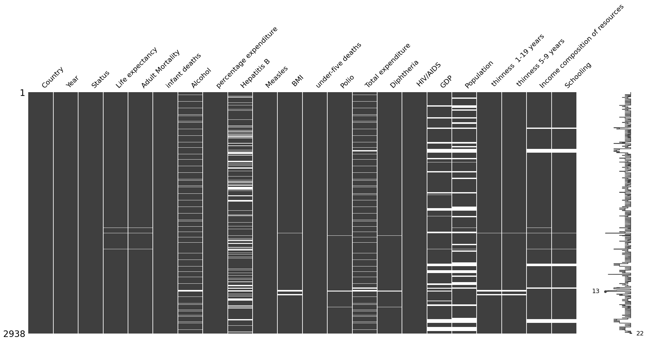
Exploratory data analysis: Missing data analysis

Let’s first inspect our data for missing values:

Your selected dataframe has 22 columns.
There are 14 columns that have missing values.

	Missing Values	% of Total Values
Population	652	22.2
Hepatitis B	553	18.8
GDP	448	15.2
Total expenditure	226	7.7
Alcohol	194	6.6
Income composition of resources	167	5.7
Schooling	163	5.5
BMI	34	1.2
thinness 1-19 years	34	1.2
thinness 5-9 years	34	1.2
Polio	19	0.6
Diphtheria	19	0.6
Life expectancy	10	0.3
Adult Mortality	10	0.3

Exploratory data analysis: Missing data analysis (continued)

Exploratory data analysis: Missing data analysis (continued)

Conclusions from analysis of missing data:

• dependent variable i.e life expectancy does not have too many missing values. Its missingness pattern seems to correlate with that of adult mortality (MAR mechanism)

• MAR mechanism at play for variables with missing values (e.g GDP, Population, Total expenditure, Alcohol, Income composition of resources, Schooling,…)

• Missingness percentage per variable low enough (highest is 22.2% for Population) that we can consider missing value imputation (especially since mechanism is MAR not MCAR!).

Exploratory data analysis

Let’s check our variable types before we go further:

data.info()

<class 'pandas.core.frame.DataFrame'>
RangeIndex: 2938 entries, 0 to 2937
Data columns (total 22 columns):
 #   Column                           Non-Null Count  Dtype  
---  ------                           --------------  -----  
 0   Country                          2938 non-null   object 
 1   Year                             2938 non-null   int64  
 2   Status                           2938 non-null   object 
 3   Life expectancy                  2928 non-null   float64
 4   Adult Mortality                  2928 non-null   float64
 5   infant deaths                    2938 non-null   int64  
 6   Alcohol                          2744 non-null   float64
 7   percentage expenditure           2938 non-null   float64
 8   Hepatitis B                      2385 non-null   float64
 9   Measles                          2938 non-null   int64  
 10   BMI                             2904 non-null   float64
 11  under-five deaths                2938 non-null   int64  
 12  Polio                            2919 non-null   float64
 13  Total expenditure                2712 non-null   float64
 14  Diphtheria                       2919 non-null   float64
 15   HIV/AIDS                        2938 non-null   float64
 16  GDP                              2490 non-null   float64
 17  Population                       2286 non-null   float64
 18   thinness  1-19 years            2904 non-null   float64
 19   thinness 5-9 years              2904 non-null   float64
 20  Income composition of resources  2771 non-null   float64
 21  Schooling                        2775 non-null   float64
dtypes: float64(16), int64(4), object(2)
memory usage: 505.1+ KB

Exploratory data analysis

• two categorical (non-numerical) variable: Status and Country

• Special and trailing characters in variable/column names (+ 1 mis-named variable ie “Thinness 1-19 years”)

Click to see the code that fixes this

import re
columns_name_fixed = []

for column in data.columns:
    if column == " thinness  1-19 years":
        column = "thinness_10_19_years"
    else:
        column = re.sub("\s|-|/","_",column.strip(" ").replace("  ", " "))
        column = column.lower()
        
    columns_name_fixed.append(column)

data.columns = columns_name_fixed
data.head() # checking processing of column names by printing first rows of dataframe

Exploratory data analysis

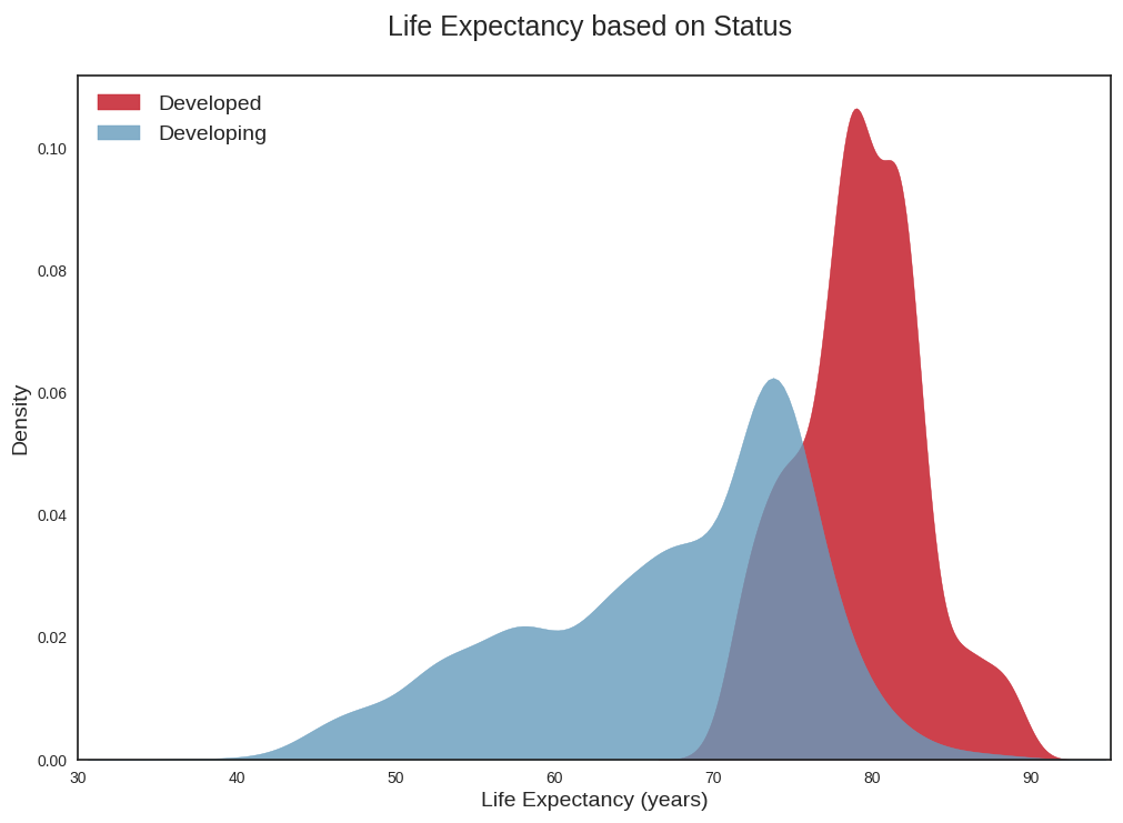
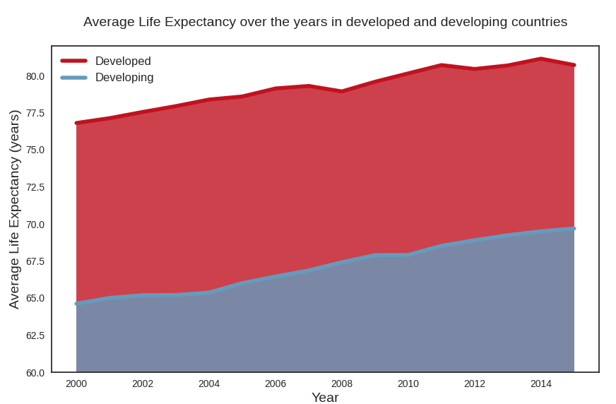
Countries categorized as ‘Developed’ have a distribution of life expectancy that is more to the right, indicating that life expectancy is higher in these countries

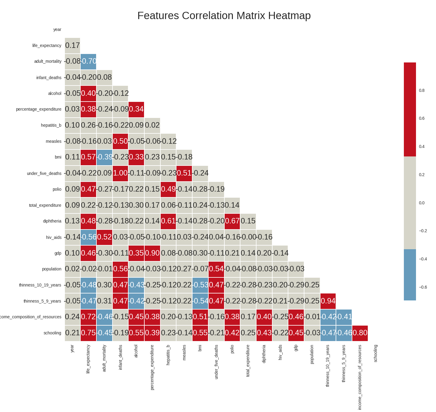
Exploratory data analysis: Variables’ correlation heatmap

• The correlation matrix shows that our target dependent variable has a high positive correlation with the features ‘schooling’, ‘income_composition_of_resources’, and ‘bmi’, and a high negative correlation with the features ‘adult_mortality’ and ‘hiv_aids’.
• The features ‘schooling’ and ‘income_composition_of_resources’ are also highly (positively) correlated, as are ‘adult_mortality’ and ‘hiv_aids’.
• Although some variables do not have a high correlation with the dependent variable, it is important to visualize these relationships graphically. That’s because the correlation heatmap only shows the Pearson correlation coefficient between variables, and therefore only allows us to visualise linear relationships between variables. This means the correlation heatmap does not allow us to capture other types of relationships that the dependent variable may have with the other variables in the dataset. ⚠️ Today, though, we’ll skip this step as we only focus on linear relationships.

Exploratory analysis: Exploring variables relationships

Exploratory analysis: Exploring variables relationships

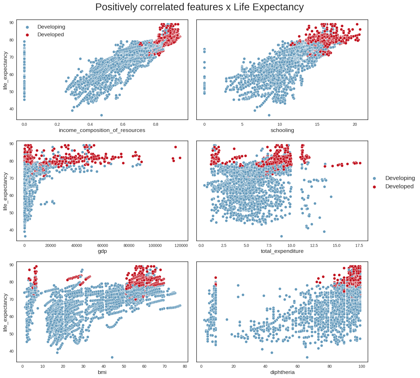
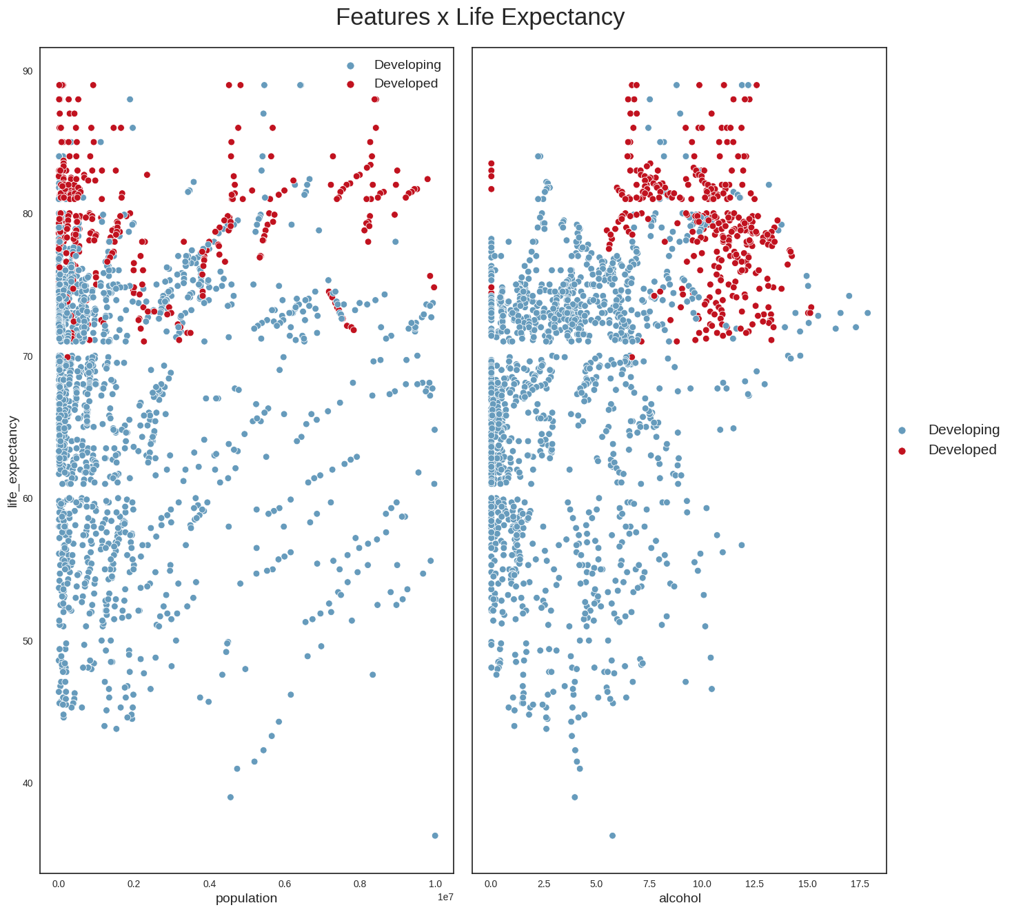
What does this mean?

• These plots have allowed us to confirm that some variables indeed do have a strong linear relationship (positive or negative) with life expectancy, e.g schooling, income_composition_of_resources, gdp, adult_mortality, hiv_aids, infant_deaths

• It seems that the absolute number of a country’s population does not directly correlated with life expectancy. A more interesting variable perhaps might be population density, which could provide more clues about a country’s social and geographical conditions.

• Another interesting point is that countries with the highest alcohol consumption also have the highest life expectancies: this looks, however, like a classic case for invoking the ‘Correlation does not imply causation’ maxim. The life expectancy of someone who owns a Ferrari is possibly higher than that of the rest of the population, but that does not mean that buying a Ferrari will increase their life expectancy. The same applies to alcohol. One hypothesis is that, in developed countries, the population has on average better financial conditions, allowing for greater consumption of luxury goods such as alcohol.

Exploratory data analysis: Variable distributions

• We have looked at the relationships of the dependent variable with the independent variables.
• Let us now analyze the distributions of these variables so that we gather initial clues as to whether there are outliers in the dataset.

Exploratory data analysis: Variable distributions

Exploratory data analysis: Variable distributions

Exploratory data analysis: Variable distributions

Exploratory data analysis

📊 Main takeways from EDA

• After the EDA, we were able to notice that the dataset seems to have a significant amount of outliers (they will have to be handled). Some of these outliers may very well be valid data, as some countries may have metrics that are very different from the others (e.g China and India, for example, have a population almost 5 times larger than the third most populous country in the world, the USA). However, we can also plausibly assert that some outliers correspond to errors during data computation: this will be better evaluated during the data cleaning stage.
• Many variables have missing values (with MAR mechanism): those missing values will have to be imputed in the data cleaning stage
• the scatter plots we built earlier showed us that our dependent variable i.e life expectancy has strong linear relationships with several of the analyzed variables.

Data cleaning: Handling of missing data

Four methods are tested:

• Mean imputation
• Median imputation
• KNN imputation
• Multiple imputation (10 iterations)

Code

import miceforest as mf
from sklearn.impute import KNNImputer
from sklearn.impute import SimpleImputer

# Dropping the `country` column
data_num = data.drop(columns='country', axis=1, inplace=False)

# Replacing the values in `status` by numerical values
data_num['status'].replace(['Developing', 'Developed'], [0, 1], inplace=True)

# KNN Imputation
imp_knn = KNNImputer()
imputed_knn = imp_knn.fit_transform(data_num)
data_imp_knn = pd.DataFrame(imputed_knn, columns=data_num.columns)

# Mean imputation
imp_mean = SimpleImputer(strategy='mean')
imputed_mean = imp_mean.fit_transform(data_num)
data_imp_mean = pd.DataFrame(imputed_mean, columns=data_num.columns)

# Median imputation
imp_median = SimpleImputer(strategy='median')
imputed_median = imp_median.fit_transform(data_num)
data_imp_median = pd.DataFrame(imputed_median, columns=data_num.columns)

# Multiple imputation
kds = mf.ImputationKernel(
  data_num,
  save_all_iterations=True,
  random_state=100
)
# Run the MICE algorithm for 10 iterations
kds.mice(10)

# Return the completed dataset.
data_imp_mice = kds.complete_data()

Data cleaning: Handling of missing data

Data cleaning: Handling of missing data

Data cleaning: Handling of missing data

Data cleaning: Handling of missing data

Data cleaning: Handling of missing data

• Here are the best imputation methods per feature based on the difference¹ of skewness and kurtosis² before and after imputation:

Imputation method	Variables it performs best for
Multiple imputation	life_expectancy, alcohol, income_composition_of_resources
KNN imputation	adult_mortality,hepatitis_b,bmi,polio, total_expenditure,diphteria,gdp,population, thinness_10_19_years,thinness_5_9_years, schooling
Mean or median imputation	N/A

• KNN or multiple imputation are the best performing imputation methods, with KNN having the edge: we’ll stick to a KNN-imputed dataset.

1. a smaller difference means the imputation performs better as it does not affect the data distribution too much

2. for a definition of skewness and kurtosis, see here

Independent variables

What could help us predict the life_expectancy variable?

Independent variables

We start by removing a few variables:

• country: our objective is to study life expectancy across various countries and not one specifically so this is not a relevant variable
• year: this variable is also not relevant for our analysis
• population: during the EDA, this variable was shown not to have a direct relationship with life_expectancy. Also, as all the other indices are computed per capita or per 1000 inhabitants, keeping this feature would only increase the complexity of our model.

Independent variables (first model)

We want to start by building a first linear regression model of life_expectancy based on a single independent variable:

• the variables with the highest correlation (positive or negative) with life_expectancy (based on EDA): schooling (0.75), income_composition_of_resources (0.72) and adult_mortality (-0.70).
• Let’s choose income_composition_of_resources for our regression (note that it is also highly correlated with schooling)

What is Linear Regression

The generic supervised model:

\[ Y = \operatorname{f}(X) + \epsilon \]

is defined more explicitly as follows ➡️

Simple linear regression

\[ \begin{align} Y = \beta_0 +& \beta_1 X + \epsilon, \\ \\ \\ \end{align} \]

when we use a single predictor, \(X\).

Multiple linear regression

\[ \begin{align} Y = \beta_0 &+ \beta_1 X_1 + \beta_2 X_2 \\ &+ \dots \\ &+ \beta_p X_p + \epsilon \end{align} \]

when there are multiple predictors, \(X_p\).

Warning

• True regression functions are never linear!
• Although it may seem overly simplistic, linear regression is extremely useful both conceptually and practically.

Linear Regression with a single predictor

We assume a model:

\[ Y = \beta_0 + \beta_1 X + \epsilon , \]

where:

• \(\beta_0\): an unknown constant that represents the intercept of the line.
• \(\beta_1\): an unknown constant that represents the slope of the line
• \(\epsilon\): the random error term (irreducible)

\(\beta_0\) and \(\beta_1\) are also known as coefficients or parameters of the model.

Linear Regression with a single predictor

We want to estimate:

\[ \hat{y} = \hat{\beta_0} + \hat{\beta_1} x \]

where:

• \(\hat{y}\): is a prediction of \(Y\) on the basis of \(X = x\).
• \(\hat{\beta_0}\): is an estimate of the “true” \(\beta_0\).
• \(\hat{\beta_1}\): is an estimate of the “true” \(\beta_1\).

The hat symbol denotes an estimated value.

Back to our case study

import numpy as np, statsmodels.api as sm
mod = sm.OLS(y_knn, X_knn)
res = mod.fit()
print(res.summary())

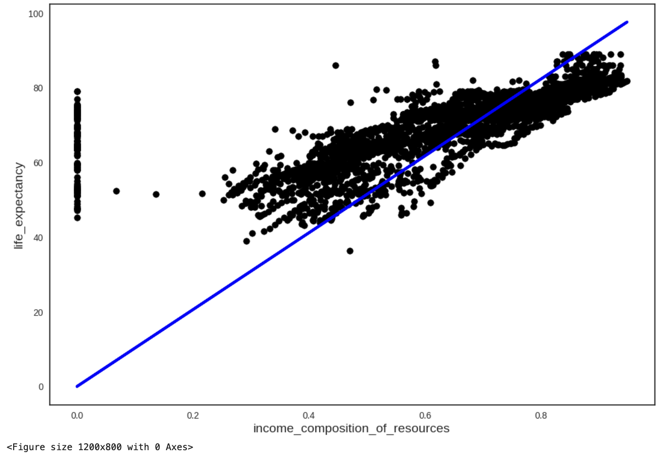
After fitting a linear model to estimate life_expectancy based on income_composition_of_resources, we are left with the following results:

• Coefficients: 102.9273
• Mean squared error (RMSE): 16.72575831404811
• Coefficient of determination (R-squared): 0.943

Our model equation is, therefore, currently:

\[\begin{align} \operatorname{life\_expectancy} = & 102.9273 \times \operatorname{income\_composition\_of\_resources} \end{align}\]

Visualising the model

What about confidence intervals?

• If we were to fit a linear model from repeated samples of the data, we would get different coefficients every time.
• Because of the Central Limit Theorem, we know that the mean of this sampling distribution can be approximated by a Normal Distribution.
• We know from Normal Theory that 95% of the distribution lies within two times the standard deviation (centred around the mean).
  

A 95% confidence interval is defined as a range of values such that with 95% probability, the range will contain the true unknown value of the parameter.

Back to our example

One can calculate the confidence intervals for the coefficients using the conf_int function from the statsmodels.api library in Python:

res.conf_int(0.05) #95% confidence interval

	2.5 %	97.5 %
income_composition_of_resources	102.009374	103.84519

Hypothesis testing

• The idea of confidence intervals is closely related to the idea of hypothesis testing.
• The most common hypothesis test involves testing the null hypothesis of:
  • \(H_0\): There is no relationship between \(X\) and \(Y\) versus the .
  • \(H_A\): There is some relationship between \(X\) and \(Y\).

• Mathematically, this corresponds to testing:

\[ \begin{align} &~~~~H_0:&\beta_1 &= 0 \\ &\text{vs} \\ &~~~~H_A:& \beta_1 &\neq 0, \end{align} \]

since if \(\beta_1=0\) then the model reduces to \(Y = \beta_0 + \epsilon\), and \(X\) and \(Y\) are not associated.

p-values

• To test the null hypothesis, we compute something called a t-statistic (a bell-shaped distribution¹)
• Using statistical software, it is easy to compute the probability of observing any value equal to \(\mid t \mid\) or larger.
• We call this probability the p-value.
• If the p-value is less than some pre-specified level of significance, say \(\alpha = 0.05\), then we reject the null hypothesis in favor of the alternative hypothesis.

1. 🤔 How are the t-distribution and the Normal distribution related? Check this link to find out.

Multivariate linear regression

Let’s fit a multivariate linear regression model to the data in our case study:

• We remove variable strongly correlated with each other (e.g we only choose one of income_composition_of_resources and schooling, one of percentage_expenditure or total_expenditure, one of gdp or percentage_expenditure, one of thinness_10_19_years or thinness_5_9_years, one of diphteria or hepatitis_b, one of infant_deaths or under_five_deaths)

• We keep the variables with strongest correlation with life_expectancy:

  • income_composition_of_resources
  • adult_mortality
  • gdp
  • hiv_aids
  • thinness_10_19_years
  • diphteria
  • bmi
  • alcohol
  • polio

Multivariate linear regression

#Select the independent variables
X_ind=data_imp_knn[['income_composition_of_resources','adult_mortality','gdp','hiv_aids','thinness_10_19_years','diphtheria','bmi','alcohol','polio']]

#Fit the model
model = sm.OLS(y_knn, X_ind)
result = model.fit()

# calculate rmse
y_predicted = result.predict(X_ind)
rmse_multivar = rmse(y_knn, y_predicted)
# Print model summary
print(result.summary())

All variables except GDP came back significant:

	coef	std err	t	P>|t|	[0.025	0.975]
income_composition_of_resources	38.9115	1.097	35.470	0.000	36.760	41.062
adult_mortality	0.0254	0.002	15.335	0.000	0.022	0.029
gdp	6.661e-07	1.54e-05	0.043	0.965	-2.95e-05	3.08e-05
hiv_aids	-0.5993	0.042	-14.288	0.000	-0.682	-0.517
thinness_10_19_years	1.0417	0.046	22.776	0.000	0.952	1.131
diphtheria	0.1472	0.010	14.226	0.000	0.127	0.168
bmi	0.2209	0.011	19.909	0.000	0.199	0.243
alcohol	0.3061	0.054	5.663	0.000	0.200	0.412
polio	0.1615	0.010	15.662	0.000	0.141	0.182

Multivariate linear regression

We remove gdp from the model and substitute total_expenditure for it (variable that was highly correlated with gdp)

This time, all variables come back significant:

	coef	std err	t	P>|t|	[0.025	0.975]
income_composition_of_resources	37.1246	1.009	36.783	0.000	35.146	39.104
adult_mortality	0.0210	0.002	13.445	0.000	0.018	0.024
total_expenditure	1.3447	0.071	18.921	0.000	1.205	1.484
hiv_aids	-0.6377	0.040	-16.097	0.000	-0.715	-0.560
thinness_10_19_years	0.9971	0.043	23.154	0.000	0.913	1.082
diphtheria	0.1252	0.010	12.733	0.000	0.106	0.144
bmi	0.1801	0.011	16.834	0.000	0.159	0.201
alcohol	0.1187	0.052	2.301	0.021	0.018	0.220
polio	0.1439	0.010	14.722	0.000	0.125	0.163

And we seemingly have a better model fit:

• higher R-squared metric than in the single predictor model: 0.983 instead of 0.943
• lower RMSE: 9.212757334610941

The model’s equation

\[\begin{align} \operatorname{life\_expectancy} = & 37.1246 \times \operatorname{income\_composition\_of\_resources} \\ & + 0.0210 \times \operatorname{adult\_mortality}\\ & + 1.3447 \times \operatorname{total\_expenditure}\\ & -0.6377 \times \operatorname{hiv\_aids} \\ & + 0.9971 \times \operatorname{thinness\_10\_19\_years} \\ & + 0.1801 \times \operatorname{bmi} \\ & + 0.1252 \times \operatorname{diphtheria} \\ & + 0.1187 \times \operatorname{alcohol} \\ & + 0.1439 \times \operatorname{polio} \end{align}\]

🤔 How should we interpret the coefficients this time?

What can go wrong?

• The model is only as good as the data you use to fit it.
• The model is only as good as the assumptions it makes.
• People forget that the level of statistical significance is somewhat arbitrary.

Indicative reading of the week:

Now for something (slightly) different

• RCTs
• A/B testing
• Causal inference

Randomised controlled trials

• A randomised controlled trial (RCT) is a type of experiment in which participants are randomly assigned to one of two or more groups (treatment and control).
• It is the norm in medicine and the life sciences, but also very common in the social sciences.
• It is deemed by some to be the gold standard for determining causality.

RCTs: how do they work?

You have a group of people

• Half of them get a pill
• The other half gets a placebo (sugar pill)

You split them into two groups at random

Then what?

• After a while, you measure the outcome of interest
• You compare the two groups using a statistical hypothesis test
• If the difference is statistically significant, you can conclude that the treatment caused the outcome

A/B testing

Causal Inference

📗 Book recommendation:

Pearl, Judea, and Dana Mackenzie. 2018. The Book of Why: The New Science of Cause and Effect. London: Allen Lane.

–(Pearl and Mackenzie 2018)

References

Aschwanden, Christie. 2015. “Science Isn’t Broken.” FiveThirtyEight. https://fivethirtyeight.com/features/science-isnt-broken/.

Enders, Craig K. 2022. Applied Missing Data Analysis. Guilford Publications.

Pearl, Judea, and Dana Mackenzie. 2018. The Book of Why: The New Science of Cause and Effect. London: Allen Lane.

Scheffer, Judi. 2002. “Dealing with Missing Data.”